Variability of the total ozone trend over Europe for the period 1950?2004 derived from reconstructed data

(1)

HAL Id: hal-00303223

https://hal.archives-ouvertes.fr/hal-00303223

Submitted on 4 Jan 2008

HAL is a multi-disciplinary open access

archive for the deposit and dissemination of sci-entific research documents, whether they are pub-lished or not. The documents may come from teaching and research institutions in France or abroad, or from public or private research centers.

L’archive ouverte pluridisciplinaire HAL, est destinée au dépôt et à la diffusion de documents scientifiques de niveau recherche, publiés ou non, émanant des établissements d’enseignement et de recherche français ou étrangers, des laboratoires publics ou privés.

Variability of the total ozone trend over Europe for the

period 1950?2004 derived from reconstructed data

J. W. Krzy?cin, J. L. Borkowski

To cite this version:

J. W. Krzy?cin, J. L. Borkowski. Variability of the total ozone trend over Europe for the period 1950?2004 derived from reconstructed data. Atmospheric Chemistry and Physics Discussions, Euro-pean Geosciences Union, 2008, 8 (1), pp.47-69. �hal-00303223�

(2)

ACPD

8, 47–69, 2008

Total ozone trend over Europe: 1950–2004 J. W. Krzy´scin and J. L. Borkowski Title Page Abstract Introduction Conclusions References Tables Figures ◭ ◮ ◭ ◮ Back Close

Full Screen / Esc

Printer-friendly Version Interactive Discussion

Atmos. Chem. Phys. Discuss., 8, 47–69, 2008 www.atmos-chem-phys-discuss.net/8/47/2008/ © Author(s) 2008. This work is licensed

under a Creative Commons License.

Atmospheric Chemistry and Physics Discussions

Variability of the total ozone trend over

Europe for the period 1950–2004 derived

from reconstructed data

J. W. Krzy ´scin and J. L. Borkowski

Institute of Geophysics, Polish Academy of Sciences, Warsaw, Poland

Received: 28 November 2007 – Accepted: 4 December 2007 – Published: 4 January 2008 Correspondence to: J. W. Krzy´scin (jkrzys@igf.edu.pl)

(3)

ACPD

8, 47–69, 2008

Full Screen / Esc

Abstract

Long-term variability of total ozone over Europe is discussed using results of a flexible trend model applied to the reconstructed total ozone data for the period 1950–2004. The data base used was built within the objectives of the COST action 726 “Long-term changes and climatology of UV radiation over Europe”. The trend pattern, which

5

comprises both anthropogenic and “natural” component, is not a priori assumed but it is a result of a smooth curve fit to the zonal monthly means and monthly grid values. The trend values in 5-year and 10-year intervals in cold (October–next year April) and warm (May–September) seasons are calculated as the differences between the smooth curve values at the end and beginning of selected time intervals divided by length of

10

the intervals. The confidence intervals for the trend values are calculated by the block bootstrapping. The statistically significant negative trends are found almost over whole Europe only in the period 1985–1994. Negative trends up to −3% per decade appeared over small areas in earlier periods when the anthropogenic forcing on the ozone layer was weak. The statistically positive trends are found only during warm seasons 1995–

15

2004 over Svalbard archipelago. The reduction of ozone level in 2004 relative to that before the satellite era is not dramatic, i.e., up to ∼−5% and ∼−3.5% in the cold and warm subperiod, respectively. Present ozone level is still depleted over many popular resorts in southern Europe and northern Africa. For high latitude regions the trend overturning could be inferred in last decade (1995–2004) as the ozone depleted areas

20

are not found there in 2004 in spite of substantial ozone depletion in the period 1985– 1994.

1 Introduction

Negative trends in the ozone content in the atmosphere in the mid- and high latitude regions over both hemisphere and anticipated increase of the surface UV radiance

25

(UVR) there triggered numerous studies on variability of UVR in different time scales 48

(4)

ACPD

8, 47–69, 2008

Full Screen / Esc

and its influencing factors including ozone, aerosols, and clouds (Bais et al., 2007, and references herein).

The time series of the surface UV-B measurements longer than 2 decades are rather rare. 14 sites in the United States were analyzed by Weatherhead et al. (1997) and only one site, Belsk, in Europe by Borkowski (2000). Length of reliable data records is

5

up to 10–15 year for most European UV observing stations. It is recognised that such period is not adequate to carry out trend analyses (Weatherhead et al., 1998). How-ever, recent studies show possibilities to reconstruct the surface UVR using variables (total ozone, cloud/aerosol optical depth) directly affecting UVR (e.g., Kaurola et al., 2000; den Outer et al., 2000; Fioletov et al., 2001) The pyranometer and other

mete-10

orological data (sunshine duration and cloud cover) serve as proxies for the combined cloud/aerosols effects on UVR. Comparison of the European UV reconstruction mod-els under the COST action 726 “Long-term changes and climatology of UV radiation over Europe” shows that past UV field can be accurately estimated using models taking into account only total ozone and pyranometric data (Koepke et al., 2006). The

recon-15

structed datasets, which can extend backward in time to as early as the beginning of total ozone and pyranometer observations, would help to examine the UVR variability over Europe in periods without UV measurements.

Observations of the total (Sun + sky) solar irradiance integrated over the whole spec-tral range (∼300–3000 nm) using pyranometers belong to standard measurements

car-20

ried out at many meteorological stations. Since the late 1970s the global distribution of ozone has been available from satellite observations. Much less is known about strato-spheric ozone during earlier periods. Current data archive centred at the World Ozone and Ultraviolet Data Center (WOUDC) in Toronto, Canada contain only few continu-ous total ozone records starting before International Geophysical Year in 1957. Thus

25

for a purpose of the surface UV reconstruction over Europe (within the framework of the COST-726 action objectives) a statistical model has been developed to simulate daily total ozone values and the ozone data base covering Europe has been built since 1 January 1950 (Krzy´scin, 2007). Here we present results concerning the long-term

(5)

ACPD

8, 47–69, 2008

Full Screen / Esc

variability of total ozone over Europe for the period 1950–2004. There were many studies focusing on trends in ozone but usually an anthropogenic component of the term variability was extracted from the data. Our objective is to estimate the long-term ozone forcing on the surface UV. Thus we calculate the trend component that comprises both the anthropogenic and “natural” effects.

5

2 Total ozone data base

Statistical model has been proposed within the framework of the COST-726 action to reproduce past total ozone variations over Europe to be used for surface UV simulation (Krzy´scin, 2007). An assimilated data base of total column ozone measurements from satellites covering the whole globe, known as NIWA total ozone data base (named after

10

affiliation of leading author Greg Bodeker – National Institute of Water and Atmosphere Research, Lauder, New Zealand) is used as input to our regression model. The NIWA data were homogenized by a comparison with the ground-based Dobson spectropho-tometer stations. The data base was widely used in various studies of global ozone behaviour (Bodeker et al., 2001 and 2005; Fioletov et al., 2002; WMO, 2003 and 2007).

15

The COST-726 ozone reconstruction model consists of two-step regression. The first step is a regression of the monthly means of NIWA total ozone on various stan-dard ozone explanatory variables, i.e., indices of the atmospheric circulation and me-teorological variables (temperature, absolute vorticity). Next is a regression of the daily departures of NIWA total ozone from the total ozone monthly means. Here, the

20

explanatory variables are deviations of daily values of meteorological variables from their monthly means. Finally, the modelled daily total ozone is obtained as a sum of terms being multiplication of regression constants and pertaining explanatory variables that were selected as important regressors using the multivariate adaptive regression splines (MARS) technique (Friedman, 1979). The quality of the data base is assured

25

by a comparison of the reconstructed total ozone with the ground-based data from several Dobson stations functioning in the early 1950s and 1960s. The model explains

(6)

ACPD

8, 47–69, 2008

Full Screen / Esc

∼70–80% variance of the ozone data collected before the satellite era. Bias and the long-term drift between the reconstructed and measured Dobson ozone are within a range of ±2%.

The reconstructed COST-726 ozone data base consists of daily total values since 1 January 1950 for a region: λ=(25.625◦W, 35.625◦E), φ=(30.5◦N, 80.5◦N). The grid

5

resolution is 1◦ in the latitudinal and 1.25◦ in the longitudinal direction (see grid struc-ture in Fig. 1). The data base is available at addresshttp:/tau.igf.edu.pl/∼_jkrzys _with

separate files describing the data format and performance of the model.

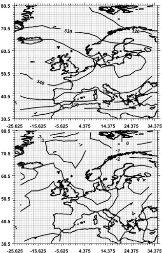
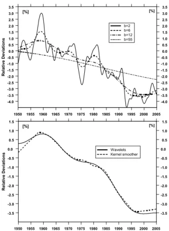
The total ozone distribution over Europe in March and July shown in Fig. 1 and Fig.2, respectively, has been calculated averaging daily total ozone values taken from the data

10

base. Top figures represent the overall long-term monthly means for the period 1950– 1959. Bottom Figures provide the departures of the overall long-term monthly means for the period 1995–2004 relative to the 1950–1959 means in percent of the latter means. A substantial ozone depletion over Europe can be inferred from a comparison between the modelled ozone means in last and first decade of analyzed data. Further

15

in the text we present results of trend analysis and visualize the spatial and temporal variability of the total ozone field over Europe.

3 Trend model

In previous studies of the total ozone trends authors focused on an extraction of com-ponent of the long-term variability being result of anthropogenic forcing (release of

20

various chemicals like freons and halogens destroying the ozone layer), Chipperfield et al. (2007) and references herein. The natural variations of total ozone were param-eterized and removed from the series, e.g. the 11-year solar signal, QBO, etc. Our approach is different when searching for the UV response to changing the ozone layer. We would like to estimate the long-term changes in total ozone comprising both

an-25

thropogenic and “natural” effects.

The long-term variability of total ozone was usually derived from a straight line fit to 51

(7)

ACPD

8, 47–69, 2008

Full Screen / Esc

the whole analyzed time series or its subsets (e.g., Reinsel et al., 2002; WMO, 2003). A comparison of slopes of the regression lines enables to infer temporal variations of the long-term trend in last decades. Recently a concept of trend evaluation using a smooth curve fit to the ozone data has been evolving (Harris et al., 2003; Krzy´scin et al., 2005; Oltmans et al., 2006; and Krzy´scin, 2006). The trend means continuing and

5

smooth change over a given time period. A difference between the curve’s values at the end and beginning of the time period divided by the length of the period gives the trend value. A model using such concept is the so-called flexible trend model and it is also used here:

∆O3(tm,K) = F (tm,K) + Noise(tm,K) (1)

10

where ∆O3(tm,K) is the relative deviation of the modeled monthly means total ozone for

calendar month m and year K relative to the long-term 1950–1978 monthly mean for month m in percent of the long-term mean, F (tm,K) represents low frequency

compo-nent, i.e., a trend component derived by smoothing of the data, Noise(t_m,K) is a noise component that is calculated as departures from the smoothed curve. The model is

15

run separately for the cold and warm subset of the year for each grid point in the area shown in Fig. 1.

Various smoothing techniques are possible, for example, wavelets, locally weighted regression (LOWES), kernel, smoothing spline, etc. These procedures could be found in the present statistical software (e.g. S-Plus 4 Guide to Statistics, 1997). The most

20

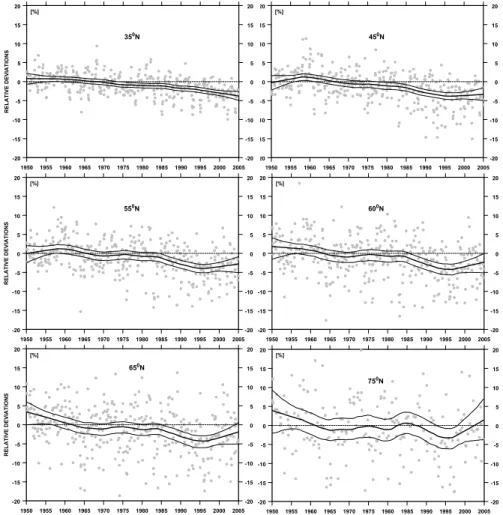
essential problem in the data smoothing for trend analysis is selection of a smoothness level, i.e., what scales of the time series variability should be retained for a trend deter-mination. The level could be arbitrarily chosen for most of presently used smoothers. For example, Fig. 3 (top) shows possible candidates for trend components extracted from an application of the kernel smoother with different temporal bandwidths (from

25

2-year up to 55-year) to the relative deviations of monthly means of total ozone for the period 1950–2004, which were averaged over the band 40◦–45◦N. It is difficult to decide which curve provides a trend component.

(8)

ACPD

8, 47–69, 2008

Full Screen / Esc

The wavelet analysis may facilitate the process of proper selection of the smooth-ness level. The wavelet multiresolution decomposition separates the series into components, and so-called “smooth” component is appropriate for trend analysis (e.g. Borkowski, 2002). Such component of the ozone time series together with the plot of the series obtained by the application of the kernel smoother with bandwidth

5

8-year are shown in Fig. 3 (bottom). In the performed multiresolution decomposition non-decimated wavelet transform was used because such a transform is translation invariant and in comparison with ordinary discrete wavelet transform provides better resolution at longer time scales (Bruce and Gao, 1996). Thus, it seems that the curve extracted by the kernel smoother with bandwidth 8-year could be treated as a trend

10

component for 55-year time series. We decide to use such kernel smoother for all ex-amined time series in spite of that wavelet smoother has some advantages over other smoother. The wavelets smoother requires equidistance data points, which are lack-ing for high latitude regions (no data durlack-ing polar night) or seasonal data (time series of monthly means for selected calendar months; cold period, October-next year April;

15

warm period, May-September).

The 95% confidence ranges for the trend curves calculated for zonal monthly means and monthly grid point values are derived here by the block bootstrapping. The boot-strap belongs to the category of nonparametric statistical methods. It is able to simulate the probability distribution of any statistics without making any assumptions related to

20

the temporal or spatial covariance structure of the variables. Resampling with replace-ment of the original record provides a sample of potential time series. However, a construction of potential representatives of the original record must preserve the tem-poral structure of the original one. In our approach many hypothetical time series of ∆O3(tm,K) are generated by a random resampling of the yearly blocks taken from

25

Noise(t_m,K) time series, Noise∗

(tm,K) = Noise(tm,K ∗) (2)

where Noise∗(t_m,K) is potential noise term in calendar month m and year K being the same as noise term in year K ∗, K ∗ is randomly selected year between 1950 and 2004.

(9)

ACPD

8, 47–69, 2008

Full Screen / Esc

The same K ∗ is used for all months in year K . Resampling of blocks of data is known as the moving-blocks bootstrap first introduced by Kunsch (1989). Noise∗(t_m,K) term is added to the original smooth curve from (1) and a new hypothetical low frequency component, F∗(tm,K), is extracted and stored. We analyze a sample of 1000 time

series of F∗(t_m,K) and calculate several statistical characteristics related to the trend

5

variability, i.e., mean change over 5-year and 10-yr intervals, value of the trend curve at the end of time series. These values are sorted in ascending order and point No. 25 and No. 975 define the 95% confidence range for the estimated values.

4 Results

The zonal monthly means are calculated averaging the daily data taken from the

COST-10

726 total ozone data base over Europe. The relative deviations for the zonal monthly means are derived as differences between the zonal monthly means and the overall monthly means for the 1950–1978 (pre-satellite era of ozone observations) expressed as percent of the overall means. The trend curves are calculated by the kernel smooth-ing with bandwidth 8-year as it was discussed in previous section. In this section we

15

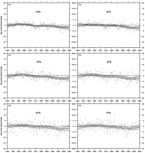
focus on behavior of the smooth curves rather than on individual monthly data. Further in the text we discuss temporal and zonal changes in the trend patterns over Europe. Figure 4 and Fig. 5 show the trend curves extracted from the relative deviations of zonal monthly means for cold (October- next year April) and warm (May-September) seasons, respectively

20

It is seen that the statistically significant negative departures of zonal mean total ozone appeared in the mid 1980s. Until the end of the analyzed period ozone stays below its pre-satellite era values. It seems that the ozone lowering stops around 1995. No further thinning of the ozone layer during the last decade (1995–2004) over Europe could be inferred from the trend curve patterns. Some insights of a trend turnaround

25

in the mid 1990s should be noted especially in higher latitudes (φ>55◦ for the cold periods, φ≥65◦for the warm period). A declining tendency could be hypothesized for

(10)

ACPD

8, 47–69, 2008

Full Screen / Esc

zonal bands with φ ≥60◦, in two decades at the beginning of ozone record, during cold seasons. The width of 95% confidence range of the trend curve is enlarged at the end and beginning of the time series and for higher latitudes regions. Thus, these findings cannot be supported by a rigorous statistical test.

The trend curve is divided into moving 5-year blocks to find a trend variability. Thus,

5

moving trend values will be calculated for time intervals: 1950–1955, 1951–1956, ..., 1998–2003, 1999–2004. The trend value (in %/10-yr.) in month t_m,K is obtained as the difference between the trend curve values in this month and that 5-year earlier divided by the length of the time interval;

Trend(tm,K) = 2(F (tm,K) − F (tm,K −5yr)) (3)

10

Figure 6 (cold seasons) and Fig. 7 (warm seasons) illustrate the trend variability for the same latitudinal bands as those used in Fig. 4 and Fig. 5. Pattern of the trend variability is similar almost in all zonal bands, i.e., maxima at the beginning, middle, and at the end of the data period, and minima in the 1960s–early 1970s, and in the 1980–early 1990s. Only the trend pattern for cold seasons in the 35◦N band suggests steadily

15

decline of total ozone throughout the whole time series. The 95% confidence range of the trend estimates increases from ±1% (±1.5%) per decade to ±2% (±4%) per decade from the lowermost to the uppermost zonal band during warm (cold) seasons. The mean trend values over the zonal bands (marked as thick line in Fig. 6 and Fig. 7) are not large, i.e., ∼−1.5% (∼−3%) per decade at the trend minima and ∼1.0% (∼3%)

20

at the trend maxima during warm (cold) seasons. Thus, statistically significant negative trends are found for small parts of the analyzed 55-yr time series, i.e., between late 1980s and mid 1990s and for shorter periods between 1960s and 1970s. Statistically significant positive trends do not appeared over the analyzed bands. However, it is worth noting large upward tendency that is manifested at the end of time series over

25

the high latitudinal regions especially during cold seasons. The trend is still negative in recent decade (1995–2004) over the 35◦N band during cold seasons.

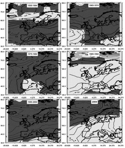
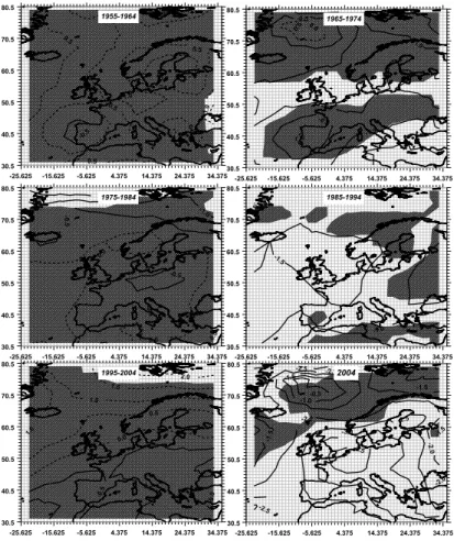
Figure 8 (cold seasons) and Fig. 9 (warm season) illustrate spatial variability of the ozone trend over Europe in decade blocks since 1955 and the ozone level at the end

(11)

ACPD

8, 47–69, 2008

Full Screen / Esc

of data (2004). The ozone time series for each grid point are analyzed, and the trend values for 10-yr blocks are calculated using the same methodology which was applied for the zonal total ozone means. Dashed regions mark areas where the estimated values are not statistically significant at 95% confidence level. The confidence limits are derived by the block bootstrapping.

5

The statistically significant negative trends are found for larger European areas only in the period 1985–1994. Some regions with negative trends appeared in earlier decades but their areas were rather limited, for example, Great Britain and the eastern part of the Mediterranean Sea in warm seasons 1965–1974, Southern France, Spain, the western part of the Mediterranean Sea, and Northern Africa in cold seasons 1975–

10

1984. The statistically positive trends are found only during warm seasons 1995–2004 over Svalbard archipelago. It is worth noting appearance of statistically significant trend in cold seasons 1994–2004 over the central/southern part of the Mediterranean Sea and Northern Africa. The ozone level at the end of time series is below pre-satellite (1978) mean level over the low and mid-latitude areas over Europe with the largest

15

decline in the southern part of Europe (∼4–5%decline during cold seasons) and cen-tral Europe (∼3–3.5% decline during warm seasons). It seems that during last two decades substantial changes in the trend pattern occurred in the high latitudes regions of Europe especially in cold seasons as the ozone depleted areas disappeared there at the end of the data that was followed by a large ozone depletion in the 1985–1995.

20

However, larger uncertainties of the statistical estimates for the high latitudes region do not allow to draw convinced (statistically significant) conclusion.

5 Summary and conclusions

Thinning ozone layer has focused interest of scientific community for almost two decades as expected increases of UVR reaching the Earth surface were linked with

25

detrimental ecological aspects. The ozone trend analyses have been targeted to esti-mation of an anthropogenic component of the ozone trend. Many efforts have been put

(12)

ACPD

8, 47–69, 2008

Full Screen / Esc

to parameterize “natural” variations in ozone (e.g. Fioletov et al., 2002; Steinbrecht et al., 2003; Dhomse et al., 2005; Wohltmann et al., 2007). Thus resulting trend pattern after elimination of the “natural” fluctuations” are thought to be an effect of the an-thropogenic forcing related to an increase of the atmosphere loading by human made substances destroying ozone layer. However, for an estimation of danger of thinning

5

ozone layer we need also information of total ozone trend pattern comprising both the anthropogenic and “natural” forcing. Here, we present an analysis of the long-term vari-ability of total ozone over Europe based on the reconstructed data extending back to 1 January 1950. The data base was built within the objective of the COST-726 project activity (Krzy´scin, 2007). The basic idea of the proposed trend model is to fit proper

10

smooth curve to the scattered monthly data and evaluation of the trend variability from the differences between the curve’s values at selected intervals. The confidence in-tervals for derived trend values are calculated by the block bootstrapping of the model residual term.

Inspection of the spatial/temporal long-term ozone variability over Europe suggests

15

significant changes of the ozone field over Europe in recent decades. The scale of ozone depletion relative to the ozone level before the satellite era of observations is not dramatic. Maximum present decline (in 2004, the end of analyzed data) of the European total ozone is not dramatic, i.e., ∼−5% and ∼−3.5% in the cold (October– next year April) and warm (May–September) subperiod of the year, respectively. The

20

statistically significant negative trends over large areas are mainly found in the mid 1980s up to mid 1995. For high latitude regions the trend overturning could be inferred in last decade (1995–2004) as the ozone depleted areas are not delineated there in 2004. It suggests a compensation of a large ozone depletion that happened before the mid 1990s over high north latitudes. Substantial thinning (up to −3%/per decade) of

25

ozone layer could be found for some areas before 1980s, for example region along the Arctic circle in 1955–1964. Thus an importance of dynamical processes in forming the long-term pattern of the ozone variability should be stressed here (see also a positive trend of ∼2% per decade over Svalbard archipelago in the 1995–2004 warm seasons).

(13)

ACPD

8, 47–69, 2008

Full Screen / Esc

It is worth mentioning from perspective of protection against excessive UVR that present total ozone level over large areas of central and southern part of continental Europe in warm season, i.e., in period with naturally high surface UVR, is still ∼3% below its level before 1980. Moreover, during cold season present ozone level is still depleted over many winter resorts over southern Europe and northern Africa. What is

5

most alarming negative trend still exist in last decade for some isolated areas there, like the southern part of the Mediterranean Sea. Thus, further public informing of danger related to the UV overexposes is still vital issue.

Acknowledgements. The study has been triggered by the COST-726 action objectives and funded by the Ministry of Sciences and Higher Education under grant No.2 P04D06728.

Au-10

thors would like to thank G. Bodeker for providing NIWA data.

References

Bais, A. F., Lubin, D., Arola, A., Bernhard, G., et al.: Surface ultraviolet radiation: past, present, and future. Chapter 7 in Scientific Assessment of Ozone Depletion: 2006, Global Ozone Re-search and Monitoring Project, Report No.50, World Meteorological Organization, Geneva,

15

Switzerland, 2007.

Bodeker, G. E., Scott, J., Kreher, K., and McKenzie, R.: Global ozone trends in potential vorticity coordinates using TOMS and GOME intercompared against the Dobson network: 1978– 1998, J. Geophys. Res., 106, 23 029–23 042, 2001.

Bodeker, G. E., Shiona, H., and Eskes, H.: Indicators of Antarctic ozone depletion, Atmos.

20

Chem. Phys., 5, 2603–2615, 2005,

http://www.atmos-chem-phys.net/5/2603/2005/.

Borkowski, J. L.: Homogenization of the Belsk UV-B time series (1976–1997) and trend analy-sis, J. Geophys. Res, 105, 4873–4878, 2000.

Borkowski, J. L.: Variations of UV-B radiation, ozone, and cloudiness at different time scale; a

25

wavelet analysis, Acta Geophys. Pol, 50, 109–117, 2002.

Bruce, A. and Gao, H.-Y.: Applied wavelet analysis with S-PLUS, Springer Verlag, New York, 1996.

(14)

ACPD

8, 47–69, 2008

Full Screen / Esc

Chipperfield, M. P., Fioletov, V. E., Bregman, B., Burrows, J., et al.: Global ozone: Past and present. Chapter 3 in Scientific Assessment of Ozone Depletion: 2006, Global Ozone Re-search and Monitoring Project, Report No.50, 572 pp, World Meteorological Organization, Geneva, Switzerland, 2007.

den Outer, P. N., Slaper H., Matthijsen J., Reinen H. A. J. M., and Tax, R.: Variability of

ground-5

level ultraviolet: model and measurement, Radiat. Protect. Dosimetry, 91, 105–110, 2000. Dhomse, S., Weber, M., and Burrows, J.: On the possible causes of recent increases in NH

total ozone from a statistical analysis of satellite data from 1979–2003, Atmos. Chem. Phys. Discuss., 5, 11 331–11 375, 2005.

Fioletov, V. E., McArthur L. J. B., Kerr J. B., and Wardle, D. I.: Long-term variations of UV-B

10

irradiance over Canada estimated from Brewer observations and derived from ozone and pyranometer measurements, J. Geophys. Res., 106, 23 009–23 028, 2001.

Fioletov, V. E., Bodeker, G. E., Miller, A. J., McPeters, R. D., and Stolarski, R.: Global and zonal total ozone variations estimated from ground-based and satellite measurements: 1964– 2000, J. Geophys. Res., 107, 4647, doi:4610.1029/2001JD001350, 2002.

15

Friedman, J. H.: Multivariate adaptive regression splines, The Annals of Statistics, 19, 1–50, 1991.

Harris, J. M., Oltmans, S. J., Bodeker, G. E., Stolarski, R., Evans, R. D., and Quincy, D. M.: Long-term variations in total ozone derived from Dobson and satellite data, Atmos. Environ., 37, 3167–3175, 2003.

20

Kaurola, J., Taalas P., Koskela T., Borkowski J., and Josefsson, W.: Long-term variations of UV-B doses at three stations in northern Europe, J. Geophys. Res., 105, 20 813–20 820, 2000.

Koepke, P., De Backer, H., Bais, A., Curylo, A., et al.: Modelling solar UV radiation in the past: Comparison of algorithms and input data, Proc. of SPIE, 6362, doi:10.1117/12.687682,

25

2006.

Krzy´scin, J. W., Jarosławski, J., and Rajewska-Wie¸ch, B.: Beginning of the ozone recovery over Europe? – Analysis of the total ozone data from ground-based observations, 1964– 2004, Ann. Geophys., 23, 1695–1695, 2005,

http://www.ann-geophys.net/23/1695/2005/.

30

Krzy´scin, J. W.: Change in ozone depletion rates beginning in the mid 1990s: trend analyses of the TOMS/SBUV merged total ozone data, 1978–2003, Ann. Geophys., 24, 493–502, 2006,

http://www.ann-geophys.net/24/493/2006/. 59

(15)

ACPD

8, 47–69, 2008

Full Screen / Esc

Krzy´scin, J. W.: Statistical reconstruction of daily total ozone over Europe 1950 to 2004, J. Geophys. Res., in press, 2007.

Kunsch, H. R.: The jacknife and the bootstrap for general stationary observations, Ann. Stat., 17(3), 1217–1241, 1989.

Oltmans, S. J., Lefohn, A. S., Harris, J. M., Galbally, I., et al.: Long-term changes in tropospheric

5

ozone, Atmos. Environ., 40, 3156–3173, 2006.

Reinsel, G. C., Weatherhead, E. C., Tiao, G. C., Miller, A. J., Nagatani, R. M., Wuebbless, D. J., and Flynn, L. E.: On detection of turnaround and recovery in trend for ozone, J. Geophys. Res., 107(D10), doi:10.1029/2001JD000500, 2002.

S-Plus 4 Guide to Statistics, Data Analysis Products Division MathSoft, Inc., Seattle,

Washing-10

ton, 1997.

Steinbrecht, W., Hassler, B., Claude, H., Winkler, P., and Stolarski, R.: Global distribution of total ozone and lower stratospheric temperature variations, Atmos. Chem. Phys., 3, 1421– 1438, 2003,

http://www.atmos-chem-phys.net/3/1421/2003/.

15

Weatherhead, E. C., Tiao, G. C., Reinsel, G. C., Frederick, J. E., DeLuisi, J. J., Choi, D., and Tam, W.: Analysis of long-term behavior of ultraviolet radiation measured by Robertson-Berger meters at 14 sites in the United States, J. Geophys. Res., 102, 8737–8754, 1997. Weatherhead, E., Reinsel, G. C., Tiao, C., Meng, X.-L., Choi, D., Cheang, W.-K., Keller, T.,

DeLuisi, J., Wuebbles, D. J., Kerr, J. B., Miller, A. J., Oltmans, S. J., and Frederick, J. E.:

20

Factors affecting the detection of trends: Statistical considerations and applications to envi-ronmental data, J. Geophys. Res., 103, 17 149–17 161, 1998.

Wohltmann, I., Lehmann, R., Rex, M., Brunner, D., and Mader, J. A.: A process-oriented regres-sion model for column ozone, J. Geophys. Res., 112, D12304, doi:10.1029/2006JD007573, 2007.

25

World Meteorological Organization (WMO): Scientific Assessment of Ozone Depletion: 2002, Global Ozone Research and Monitoring Project, Report No. 47, Geneva, Switzerland, 2003. World Meteorological Organization (WMO): Scientific Assessment of Ozone Depletion: 2006,

Global Ozone Research and Monitoring Project, Report No.50, World Meteorological Orga-nization, Geneva, Switzerland, 2007.

30

(16)

ACPD

8, 47–69, 2008

Full Screen / Esc

Printer-friendly Version Interactive Discussion -25.625 -15.625 -5.625 4.375 14.375 24.375 34.375 30.5 40.5 50.5 60.5 70.5 80.5 340 350 360 370 38₀ 390 40₀ 410 -25.625 -15.625 -5.625 4.375 14.375 24.375 34.375 30.5 40.5 50.5 60.5 70.5 80.5 -7 -7 -7 -6 -6 -6 -6 -5 -5 -5 -5 -4 -4 -4 -4 -4

Fig. 1. Mean total ozone (in DU) in March for the period 1950–1959 (top), the difference

between the mean total ozone in March for the period 1995–2004 and that for the period 1950– 1959 in percent of the latter means (bottom).

(17)

ACPD

8, 47–69, 2008

Full Screen / Esc

Printer-friendly Version Interactive Discussion -25.625 -15.625 -5.625 4.375 14.375 24.375 34.375 30.5 40.5 50.5 60.5 70.5 80.5 310 320 320 330 330 340 35 0 -25.625 -15.625 -5.625 4.375 14.375 24.375 34.375 30.5 40.5 50.5 60.5 70.5 80.5 -4 -4 -3 -3 -2 -2 -2 -1 -1 0

Fig. 2. Same as Fig. 1 but the mean total ozone in July is analyzed.

(18)

ACPD

8, 47–69, 2008

Full Screen / Esc

Printer-friendly Version Interactive Discussion 1950 1955 1960 1965 1970 1975 1980 1985 1990 1995 2000 2005 -4.0 -3.5 -3.0 -2.5 -2.0 -1.5 -1.0 -0.5 0.0 0.5 1.0 1.5 2.0 2.5 3.0 3.5 -4.0 -3.5 -3.0 -2.5 -2.0 -1.5 -1.0 -0.5 0.0 0.5 1.0 1.5 2.0 2.5 3.0 3.5 R e la ti v e D e v ia ti o n s [%] [%] b=2 b=6 b=12 b=55 1950 1955 1960 1965 1970 1975 1980 1985 1990 1995 2000 2005 -3.5 -3.0 -2.5 -2.0 -1.5 -1.0 -0.5 0.0 0.5 1.0 1.5 -3.5 -3.0 -2.5 -2.0 -1.5 -1.0 -0.5 0.0 0.5 1.0 1.5 R e la ti v e D e v ia ti o n s [%] [%] Wavelets Kernel smoother

Fig. 3. Smooth pattern of the zonal means of total ozone for the 40◦

–45◦N latitudinal band, application of the kernel smoother with different temporal (in years) bandwidth b (a), a smooth component of the wavelet multiresolution decomposition, and the kernel smoother with b=8-year (b).

(19)

ACPD

8, 47–69, 2008

Full Screen / Esc

Printer-friendly Version Interactive Discussion 1950 1955 1960 1965 1970 1975 1980 1985 1990 1995 2000 2005 -20 -15 -10 -5 0 5 10 15 20 -20 -15 -10 -5 0 5 10 15 20 R E L A T IV E D E V IA T IO N S [%] 350_N 1950 1955 1960 1965 1970 1975 1980 1985 1990 1995 2000 2005 20 15 10 -5 0 5 10 15 20 -20 -15 -10 -5 0 5 10 15 20 [%] 450_N 1950 1955 1960 1965 1970 1975 1980 1985 1990 1995 2000 2005 -20 -15 -10 -5 0 5 10 15 20 -20 -15 -10 -5 0 5 10 15 20 R E L A T IV E D E V IA T IO N S [%] 550_N 1950 1955 1960 1965 1970 1975 1980 1985 1990 1995 2000 2005 -20 -15 -10 -5 0 5 10 15 20 -20 -15 -10 -5 0 5 10 15 20 R E L A T IV E D E V IA T IO N S [%] 650_N 1950 1955 1960 1965 1970 1975 1980 1985 1990 1995 2000 2005 -20 -15 -10 -5 0 5 10 15 20 -20 -15 -10 -5 0 5 10 15 20 [%] 600_N 1950 1955 1960 1965 1970 1975 1980 1985 1990 1995 2000 2005 -20 -15 -10 -5 0 5 10 15 20 -20 -15 -10 -5 0 5 10 15 20 [%] 750_N

Fig. 4. Relative deviations of zonal monthly means in cold seasons (October–next year April)

and the trend curve derived by the kernel smoother for various latitudinal belts in Europe. 64

(20)

ACPD

8, 47–69, 2008

Full Screen / Esc

Printer-friendly Version Interactive Discussion 1950 1955 1960 1965 1970 1975 1980 1985 1990 1995 2000 2005 -20 -15 -10 -5 0 5 10 15 20 -20 -15 -10 -5 0 5 10 15 20 R E L A T IV E D E V IA T IO N S [%] 350_N 1950 1955 1960 1965 1970 1975 1980 1985 1990 1995 2000 2005 -20 -15 -10 -5 0 5 10 15 20 -20 -15 -10 -5 0 5 10 15 20 [%] 450_N 1950 1955 1960 1965 1970 1975 1980 1985 1990 1995 2000 2005 -20 -15 -10 -5 0 5 10 15 20 -20 -15 -10 -5 0 5 10 15 20 R E L A T IV E D E V IA T IO N S [%] 550_N 1950 1955 1960 1965 1970 1975 1980 1985 1990 1995 2000 2005 -20 -15 -10 -5 0 5 10 15 20 -20 -15 -10 -5 0 5 10 15 20 [%] 600_N 1950 1955 1960 1965 1970 1975 1980 1985 1990 1995 2000 2005 -20 -15 -10 -5 0 5 10 15 20 -20 -15 -10 -5 0 5 10 15 20 R E L A T IV E D E V IA T IO N S [%] 650_N 1950 1955 1960 1965 1970 1975 1980 1985 1990 1995 2000 2005 -20 -15 -10 -5 0 5 10 15 20 -20 -15 -10 -5 0 5 10 15 20 [%] 750_N

Fig. 5. Same as Fig. 4 but for zonal means in warm seasons (May–September).

(21)

ACPD

8, 47–69, 2008

Full Screen / Esc

Printer-friendly Version Interactive Discussion 1950 1955 1960 1965 1970 1975 1980 1985 1990 1995 2000 2005 -4 -3 -2 -1 0 1 2 3 4 -4 -3 -2 -1 0 1 2 3 4 T R E N D [ % /1 0 Y R . ] 350_N 1950 1955 1960 1965 1970 1975 1980 1985 1990 1995 2000 2005 -4 -3 -2 -1 0 1 2 3 4 -4 -3 -2 -1 0 1 2 3 4 450N 1950 1955 1960 1965 1970 1975 1980 1985 1990 1995 2000 2005 -4 -3 -2 -1 0 1 2 3 4 -4 -3 -2 -1 0 1 2 3 4 T R E N D [ % /1 0 Y R . ] 550_N 1950 1955 1960 1965 1970 1975 1980 1985 1990 1995 2000 2005 -4 -3 -2 -1 0 1 2 3 4 -4 -3 -2 -1 0 1 2 3 4 [ ] 600N 1950 1955 1960 1965 1970 1975 1980 1985 1990 1995 2000 2005 -4 -3 -2 -1 0 1 2 3 4 -4 -3 -2 -1 0 1 2 3 4 T R E N D [ % /1 0 Y R . ] 650_N 1950 1955 1960 1965 1970 1975 1980 1985 1990 1995 2000 2005 -4 -3 -2 -1 0 1 2 3 4 -4 -3 -2 -1 0 1 2 3 4 [ ] 750_N

Fig. 6. Trends (%/per decade) in 5-yr moving blocks in cold seasons – thick curve. Thin curves

show the range of 95% confidence interval. Arrows mark periods with statistically significant trend values.

(22)

ACPD

8, 47–69, 2008

Full Screen / Esc

Printer-friendly Version Interactive Discussion 1950 1955 1960 1965 1970 1975 1980 1985 1990 1995 2000 2005 -4 -3 -2 -1 0 1 2 3 4 -4 -3 -2 -1 0 1 2 3 4 T R E N D [ % /1 0 Y R . ] 350_N 1950 1955 1960 1965 1970 1975 1980 1985 1990 1995 2000 2005 -4 -3 -2 -1 0 1 2 3 4 -4 -3 -2 -1 0 1 2 3 4 450N 1950 1955 1960 1965 1970 1975 1980 1985 1990 1995 2000 2005 -4 -3 -2 -1 0 1 2 3 4 -4 -3 -2 -1 0 1 2 3 4 T R E N D [ % /1 0 Y R . ] 550_N 1950 1955 1960 1965 1970 1975 1980 1985 1990 1995 2000 2005 -4 -3 -2 -1 0 1 2 3 4 -4 -3 -2 -1 0 1 2 3 4 600_N 1950 1955 1960 1965 1970 1975 1980 1985 1990 1995 2000 2005 -4 -3 -2 -1 0 1 2 3 4 -4 -3 -2 -1 0 1 2 3 4 T R EN D [ % /1 0 Y R . ] 650_N 1950 1955 1960 1965 1970 1975 1980 1985 1990 1995 2000 2005 -4 -3 -2 -1 0 1 2 3 4 -4 -3 -2 -1 0 1 2 3 4 750_N

Fig. 7. Same as Fig. 6 but for the zonal means in warm season.

(23)

ACPD

8, 47–69, 2008

Full Screen / Esc

Printer-friendly Version Interactive Discussion -25.625 -15.625 -5.625 4.375 14.375 24.375 34.375 30.5 40.5 50.5 60.5 70.5 80.5 -3.5 -3 .0 -3.0 -3.0 -2.5 -2.5 -2.0 -1.5 -1.0 -1.0 -0.5 -0.5 -0.5 0.0 0.0 0.5 0.5 1955-1964 -25.625 -15.625 -5.625 4.375 14.375 24.375 34.375 30.5 40.5 50.5 60.5 70.5 80.5 -1_.5 -1.0 -1_.0 -1.0 -0.5 -0_.5 0.0 0.5 1.0 1.5 2.0 2.5 1965-1974 -25.625 -15.625 -5.625 4.375 14.375 24.375 34.375 30.5 40.5 50.5 60.5 70.5 80.5 -1.5 -1.0 -1.0 -1.0 -0 .5 -0.5 -0.5 0.0 0.0 0.0 0 .5 1.0 1.0 1975-1984 -25.625 -15.625 -5.625 4.375 14.375 24.375 34.375 30.5 40.5 50.5 60.5 70.5 80.5 -6.0 -5.5 -5.0 -4.5 -4.0 -3.5 -3.0 -2.5 -2_.5 -2.0 -1.5 -1.0 -1.0 1985-1994 -25.625 -15.625 -5.625 4.375 14.375 24.375 34.375 30.5 40.5 50.5 60.5 70.5 80.5 -5_.0 -4.5 -4.0 -3_.5 -3.0 -3. 0 -2.5 -2 .5 -2.0 -1.5 -1.0 -0.5 -0.5 0.0 0.0 0.5 1.0 2004 -25.625 -15.625 -5.625 4.375 14.375 24.375 34.375 30.5 40.5 50.5 60.5 70.5 80.5 -1.5 -1.0 -0.5 0.0 0.5 1.0 1.5 2.0 2.5 3.0 3.5 4.0 1995-2004

Fig. 8. Trends in 10-yr disjoined blocks (% per decade), and the relative deviation of total ozone

in 2004 (in % of ozone value in pre-satellite era) for cold season. The dashed area marks region where values are not statistically significant at 95% confidence level.

(24)

ACPD

8, 47–69, 2008

Full Screen / Esc

Printer-friendly Version Interactive Discussion -25.625 -15.625 -5.625 4.375 14.375 24.375 34.375 30.5 40.5 50.5 60.5 70.5 80.5 -0.5 0.0 0.0 0.0 0.5 0.5 0.5 0.5 0.5 1.0 1.0 1955-1964 -25.625 -15.625 -5.625 4.375 14.375 24.375 34.375 30.5 40.5 50.5 60.5 70.5 80.5 -1_.0 -1.0 -1.0 -0.5 -0.5 0.0 0.0 0.5 1965-1974 -25.625 -15.625 -5.625 4.375 14.375 24.375 34.375 30.5 40.5 50.5 60.5 70.5 80.5 -1.5 -1_.0 -0_.5 -0 .5 -0 .5 -0.5 0.0 0.0 0.0 1975-1984 -25.625 -15.625 -5.625 4.375 14.375 24.375 34.375 30.5 40.5 50.5 60.5 70.5 80.5 -1_.5 -1.0 -1 .0 1985-1994 -25.625 -15.625 -5.625 4.375 14.375 24.375 34.375 30.5 40.5 50.5 60.5 70.5 80.5 -0.5 -0.5 -0.5 0.0 0.5 1.0 1.0 1.5 2.0 1995-2004 -25.625 -15.625 -5.625 4.375 14.375 24.375 34.375 30.5 40.5 50.5 60.5 70.5 80.5 -3.5 -3.0 -2.5 -2.5 -2.5 -2.0 -2 .0 -2.0 -2.0 -1.5 -1.5 -1.5 -1.5 -1.0 -0.5 2004

Fig. 9. Same as 8 but for warm season.