Large-scale atmospheric circulation biases and changes in global climate model simulations and their importance for regional climate scenarios: a case study for West-Central Europe

(1)

HAL Id: hal-00301727

https://hal.archives-ouvertes.fr/hal-00301727

Submitted on 25 Aug 2005

HAL is a multi-disciplinary open access

archive for the deposit and dissemination of sci-entific research documents, whether they are pub-lished or not. The documents may come from teaching and research institutions in France or abroad, or from public or private research centers.

L’archive ouverte pluridisciplinaire HAL, est destinée au dépôt et à la diffusion de documents scientifiques de niveau recherche, publiés ou non, émanant des établissements d’enseignement et de recherche français ou étrangers, des laboratoires publics ou privés.

Large-scale atmospheric circulation biases and changes

in global climate model simulations and their

importance for regional climate scenarios: a case study

for West-Central Europe

A. P. van Ulden, G. J. van Oldenborgh

To cite this version:

A. P. van Ulden, G. J. van Oldenborgh. Large-scale atmospheric circulation biases and changes in global climate model simulations and their importance for regional climate scenarios: a case study for West-Central Europe. Atmospheric Chemistry and Physics Discussions, European Geosciences Union, 2005, 5 (4), pp.7415-7455. �hal-00301727�

(2)

ACPD

5, 7415–7455, 2005 Circulation biases and changes in global climate models

A. P. van Ulden and G. J. van Oldenborgh Title Page Abstract Introduction Conclusions References Tables Figures J I J I Back Close

Full Screen / Esc

Print Version Interactive Discussion

Atmos. Chem. Phys. Discuss., 5, 7415–7455, 2005 www.atmos-chem-phys.org/acpd/5/7415/

SRef-ID: 1680-7375/acpd/2005-5-7415 European Geosciences Union

Atmospheric Chemistry and Physics Discussions

Large-scale atmospheric circulation

biases and changes in global climate

model simulations and their importance

for regional climate scenarios: a case

study for West-Central Europe

A. P. van Ulden and G. J. van Oldenborgh

Koninklijk Nederlands Meteorologisch Institutuut (KNMI), PO Box 201, 3730 AE, De Bilt, Netherlands

Received: 1 June 2005 – Accepted: 24 June 2005 – Published: 25 August 2005 Correspondence to: A. P. van Ulden (aad.van.ulden@knmi.nl)

(3)

ACPD

Full Screen / Esc

Print Version Interactive Discussion Abstract

The credibility of regional climate change predictions for the 21st century depends on the ability of climate models to simulate global and regional circulations in a realistic manner. To investigate this issue, a large set of global coupled climate model experi-ments prepared for the Fourth Assessment Report of the Intergovernmental Panel on 5

Climate Change has been studied. First we compared 20th century model simulations of longterm mean monthly sea level pressure patterns with ERA-40. We found a wide range in performance. Many models performed well on a global scale. For northern midlatitudes and Europe many models showed large errors, while other models simu-lated realistic pressure fields.

10

Next we focused on the monthly mean climate of West-Central Europe in the 20th century. In this region the climate depends strongly on the circulation. Westerlies bring temperate weather from the Atlantic Ocean, while easterlies bring cold spells in winter and hot weather in summer. In order to be credible for this region, a climate model has to show realistic circulation statistics in the current climate, and a response of tempera-15

ture and precipitation variations to circulation variations that agrees with observations. We found that even models with a realistic mean pressure pattern over Europe still showed pronounced deviations from the observed circulation distributions. In partic-ular, the frequency distributions of the strength of westerlies appears to be difficult to simulate well. This contributes substantially to biases in simulated temperatures and 20

precipitation, which have to be accounted for when comparing model simulations with observations.

Finally we considered changes in climate simulations between the end of the 20th century and the end of the 21st century. Here we found that changes in simulated circulation statistics play an important role in climate scenarios. For temperature, the 25

warm extremes in summer and cold extremes in winter are most sensitive to changes in circulation, because these extremes depend strongly on the simulated frequency of eastery flow. For precipitation, we found that circulation changes have a substantial

(4)

ACPD

Full Screen / Esc

influence, both on mean changes and on changes in the probability of wet extremes and of long dry spells. Because we do not know how reliable climate models are in their predictions of circulation changes, climate change predictions for Europe are as yet uncertain in many aspects.

1. Introduction 5

Global coupled climate models are indispensible tools in climate analysis. Such models are credible if they are able to produce realistic simulations of large scale patterns of the atmospheric circulation and of other climate variables. An assessment of the per-formance of global coupled models can be found in the Third Assessment Report of IPCC (IPCC 2001), and in Achuta Rao et al. (2004). Recently many new coupled model 10

simulations have been made, both for the 20th century climate and for various future emission scenarios. Model output has been made accessible for analysis by external groups, in preparation for the Fourth Assessment Report of IPCC (see Acknowledge-ments and Table 1). This has created a unique opportunity to compare simulations by many different models with observations, and to compare climate change projections 15

by these models.

This paper deals primarily with the monthly mean climate in West-Central Europe. In this region the climate depends strongly on the atmospheric circulation. Westerlies carry maritime air from the Atlantic Ocean to the continent, while easterlies bring cold weather in winter and hot weather in summer. In order to be credible for this region, a 20

climate model has to show realistic circulation statistics in the current climate. A first requirement is that a model is able to simulate the mean circulation over the globe and over Europe in a realistic manner. Biases in the mean circulation are indications for important model deficiencies, such as a poor representation of the frequency of at-mospheric blockings (D’Andrea et al., 1998) or less credible thermohaline circulations 25

(Thorpe, 2005). Therefore, we start our analysis with a comparison of model simula-tions of longterm mean monthly sea level pressure patterns with global and regional

(5)

ACPD

Full Screen / Esc

observations. This comparison is presented in Sect. 2. Based on this test we selected a sub-set of models which show relatively realistic mean pressurre patterns over the globe and over Europe for further analysis of the climate in West-Central Europe.

For the description of regional circulation statistics, we use three geostrophic flow indices: the two components of the geostrophic wind and the geostrophic vorticity. 5

Variations in such flow indices have been shown to correlate well with variations in monthly mean temperatures and precipitation (Turnpenny et al., 2002; Van Oldenborgh and van Ulden, 2003; Van Ulden et al., 2005). In Sect. 3 we compare 20th century model simulations of these flow indices with observations in West-Central Europe. In addition we will compare observed relations between circulation on the one hand, and 10

temperature and precipitation on the other hand with the corresponding relations in the model simulations. This serves as a further test on the internal consistency of the model simulations. This analysis provides also an estimate of the contribution of biases in simulated circulations to biases in mean temperature and mean precipitation.

In Sect. 4 we analyse simulated changes in the atmospheric circulation, primarily 15

for the SRES A2 emission scenario. Using the techniques developed in Sect. 3, we will estimate the contribution of mean circulation changes to changes in temperature and precipitation. This is an important issue in the development of regional climate change scenarios, as has been shown by Jylh ¨a et al. (2004). Further, we will explore the influence of changes in the circulation statistics on changes in the distributions of 20

monthly mean temperature and precipitation.

We conclude this paper with a discussion on the complex role of atmospheric circu-lation statistics in regional climate simucircu-lations (Sect. 5).

2. Global and regional patterns of longterm mean sea level pressure

In this section we analyse longterm averages of monthly sea level pressure patterns. 25

For the validation of simulated sea level pressure patterns we use data from ERA-40 (K ˚allberg et al., 2004). In a recent paper Bromwich and Fogt (2004) found that ERA-40

(6)

ACPD

Full Screen / Esc

is not well constrained by observations in data-sparse regions of the Southern Hemi-sphere during the presatellite era. Therefore we used ERA-40 data starting from 1973. The average pressure patterns before 1973 are however very similar to the average patterns thereafter. This is probably due to a realistic climatological behaviour of the ERA-40 model. Using ERA-40 data has the added advantage, that ERA-40 deals 5

with orography in a similar manner as climate models do. Thus, there is no reason to exclude mountanous regions from the comparison. For the validation over Europe we used the ADVICE pressure reconstruction by Jones et al. (1999), which is directly based on observations in the period 1780–1995. From the model simulations we used the average of all available members of the 20th century runs. For each month these 10

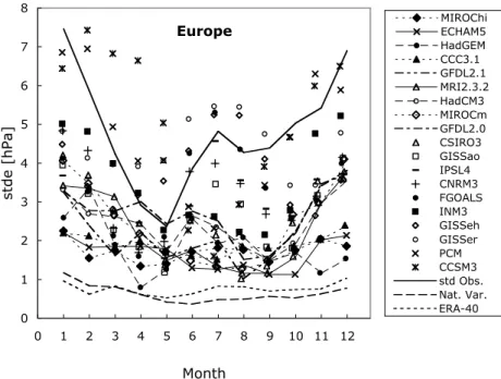
ensemble mean patterns were compared with observations for the globe, for the tropics (30◦S–30◦N), for southern latitudes (30◦S–90◦S), for northern latitudes (30◦N–90◦N) and for Europe ( 30◦W–40◦E, 35◦N–65◦N). The European domain includes Iceland and the Azores and thus comprises an important part of the North Atlantic (see Fig. 2). In Fig. 1 we present the spatial standard deviations of the difference fields between 15

simulated and observed pressure patterns for Europe. We see a wide range in model performence. In order to judge the quality of the models it is useful to look at the explained spatial variance, which is defined as:

V ARexpl = 1 − V ARdif f /V ARobs . (1)

If for a given model the standard deviation of the difference field is larger than the stan-20

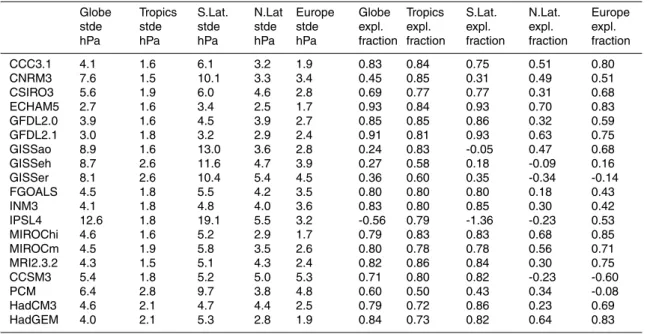
dard deviation of the observed field, the explained variance is negative for that model. In Table 2, we show the annual rms-values of the 12 monthly spatial standard devia-tions and the annual averages of the explained variance for each month. We see that for the tropics all models explain more than 50% of the spatial variance. For southern latitudes 6 models have a poor performance. This is due to unrealistics pressure fields 25

over Antarctica. The pressure fields for northern latitudes appear to be most difficult to simulate. Only 5 models explain more than 50% of the spatial variance. Important bias regions are the North Atlantic and the Asian continent. Many models have a poor performance over Europe as well.

(7)

ACPD

Full Screen / Esc

Except for Europe, the above comparison is based on a rather short observation record, so it is possible that natural variability plays a role in this comparison. Unfortu-nately we have no reliable long observation records for the global pressure fields. For Europe, however we can use the long observation record to study natural variability. It appears that individual 30 y mean fields differ less than 1 hPa from the longterm mean 5

field (Fig. 1). Also the difference between ERA-40 and the long analysed record is less than 1 hPa for all months (Fig. 1). This indicates that a 30 y year averaging period is suf-ficient to remove most of the natural variability in the European pressure patterns, and that differences caused by different analysis methods are smaller than the systematic errors in global model simulations.

10

Another important issue concerns the spatial scales of the longterm mean bias pat-terns. It appears that the dominant scales are very large: i.e. thousands of kilometers. This is important for climate simulations by high resolution regional models which have to use boundary conditions from global models. If the global model has a large-scale bias, it is likely that the regional model will inherit much of this bias (Van Ulden et al., 15

2005).

3. The 20th-century climate in West-Central Europe

3.1. Matching scales, selection of observations and selection of models

Our test domain in West-Central Europe is shown in Fig. 2. The domain is situated north of the Alps. The climate is under the influence of prevailing westerlies and mod-20

erately maritime. The geostrophic flow indices were computed in the area 0◦–20◦E, 45◦–55◦N. The geostrophic wind was computed from the sea level pressures at the four corners of the domain, using a fixed value for the air density (1.2 kgm−3). For the geostrophic vorticity we used the difference between the mean pressure at the four corners of the domain and the pressure in the center as a simple proxy. The locations 25

(8)

ACPD

Full Screen / Esc

details of procedures for the reduction of surface pressure do not play an important role. The ADVICE pressure analysis (Jones et al., 1999) was used as observation. Since this analysis has a 5◦lat × 10◦lon resolution, the pressure fields simulated by the climate models were smoothed to match this resolution. We tested the smoothing pro-cedure by comparing the smoothed ERA-40 fields with the ADVICE fields and found 5

an excellent agreement, both with respect to the mean indices and with respect to their variability. Thus we used smoothed ERA-40 data to extend the ADVICE analysis to the year 2000.

For temperature and precipitation we used the region 6◦–14◦E, 48.5◦–53.5◦N as test domain. This land domain includes a major part of Germany and smaller parts of adja-10

cent countries. The domain is at a suitable distance from the Alps and is characterised by flat plains and modest orography. Model output was averaged over this domain. This removes the direct impact of differences in model resolution, which ranges from about 120 km to 440 km in West-Central Europe.

Temperature observations for the full 20th century were taken from the updated 0.5◦ 15

gridded data set by New et al. (1999; 2000). We compared the temperatures in this data set with ERA-40 for the ERA-40 period and found an excellent agreement.

Precipitation data were also taken from New et al. (1999, 2000). This data set was not corrected for undercatchment due to snow and wind. In order to obtain an esti-mate of this undercatchment, we compared the New et al. (2000) data with a detailed 20

calibrated precipitation data set for the German part of the river Rhine basin (Van den Hurk et al., 2005). This data set covers most of the western half of our test region and is available for 1961–1995. In the overlapping domain and overlapping time period, the monthly mean precipitations of the two data sets were highly correlated (r=0.95). The comparison indicated a significant undercatchment in the New et al. data set, ranging 25

from about 2% in summer months to 20% in winter months. We corrected the New et al. (2000) data using this estimate of undercatchment in our full test domain.

For the model validation given hereafter, we selected the 8 models with the highest skill for the simulated sea level pressure fields in the European domain, as given in

(9)

ACPD

Full Screen / Esc

Table 2. For comparison, we have also included 2 models with a poor performance. We included only the first ensemble member of each 20th-century model simulation in our analysis.

3.2. Geostrophic flow statistics in the 20th century

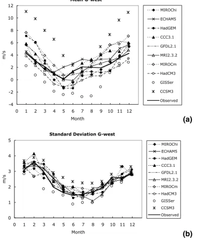
In Fig. 3 we show the mean and the standard deviation of the west-component of the 5

geostrophic wind for each month of the year. Most models have a mean westerly bias in winter, which is quite extreme for CCSM3. This positive bias is caused by a deeper than observed Icelandic low and a positive pressure bias over the Mediterranean. In summer most models have a negative (i.e. easterly) bias in G-west. GISSer even has a pronounced mean easterly flow in summer. This negative bias is caused by a high 10

pressure bias over Northern Europe and a low pressure bias over the Mediterranean. The standard deviations are relatively well modelled. The importance of biases in G-west can be further illustrated by looking at the frequency distributions.

In Fig. 4a we show the cumulative frequency distributions for G_W in January. Winter months with a mean flow from the east are characterised by cold and dry continental 15

weather. Thus the frequency of such months is an important ingredient of the winter climate. We see that GISSer overpredicts this frequency. HadGEM has a pronounced westerly bias in January, but still has a significant overlap with the observed distribution. The westerly bias in the CCSM3 simulation is very large, and the simulated distribution has little overlap with the observed distribution.

20

In Fig. 4b we show the cumulative frequency distributions for G_W in July. Summer months with a mean easterly flow have predominently warm and dry weather. About 10% of the observed July months have a mean flow from the east. Most models simu-late a much higher percentage. For GISSer all months have a mean flow from the east. On the other hand, ECHAM5 has a weak westerly bias in summer.

25

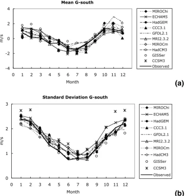
The model simulations of the south component of the geostrophic wind are relatively close to the observations and to each other, as is shown in Fig. 5.

(10)

simu-ACPD

Full Screen / Esc

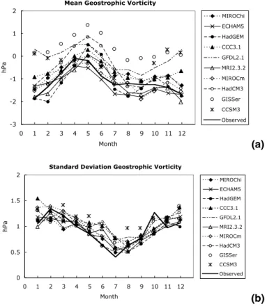
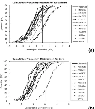
late a higher than observed mean geostrophic vorticity, and in summer a higher than observed standard deviation. In Fig. 7 the cumulative frequency distributions for Jan-uary and July are given. GISSer deviates most from the observations, in particular in July. The distribution for July simulated by this model has no overlap with the observed distribution.

5

These results show that biases in the simulated geostrophic flow indices are quite large, even for models which produce relatively realistic pressure fields over Europe. We may expect that these biases have an impact on simulations of temperature and precipitation. In the next sections we will investigate the importance of these impacts. 3.3. Relations between circulation variations and temperature variations

10

Interannual variability of the atmospheric circulation is a prime source for variability in monthly mean temperature and precipitation (Turnpenny et al., 2002; Van Oldenborgh and van Ulden, 2003). Relations between circulation on the one hand, and temperature and precipitation on the other hand, can be used to analyse the influence of differences in circulation statistics on mean temperatures and precipitation, and on their variability. 15

For the description of the influence of the circulation on temperature, we use a simple linear model. Monthly Circulation Temperature Anomalies are defined as:

CT A= A_S∆G_S + A_W∆G_W + A_V∆G_V + M (2)

where∆G_S , ∆G_W and ∆G_V are circulation anomalies relative to the mean observed values for the 20th century and where M is a memory term for past circulations. This 20

term is modeled as an exponentially decaying memory with τ as e-folding period. We retained the memory for the circulation in the previous 3 months. Monthly values of the numerical coefficients A_S , A_W , A_V and the memory τ were obtained from a least-square fit for the observations of the 20th century. We then multiplied the numerical coefficients by a scaling factor, such that the monthly CTA had the same variance 25

as the observed temperatures. Thus CTA is a variance conserving regression to the observations.

(11)

ACPD

Full Screen / Esc

This simple model performs quite well, with correlations around 0.8 (see Fig. 9). In winter and summer G_W is the dominating term in Eq. (2). In the transition months G_S and G_V give the largest contribution to the explained variance. The memory length varies typically between 0.3 m and 0.9 m. The contribution of the memory term to the explained variance is significant in late winter (memory for snow feedback) and in late 5

summer (memory for soil moisture depletion). Nearby seas produce memory effects all year round.

For the models the circulation anomalies are computed from modeled values of∆G_S, ∆GW, and∆GV using Eq. (2) and the observed values of AS, AW, AV, and the memory

τ. The variance conserving regression line for simulated temperature anomalies is

10

given by:

T A_Regr.=< T A > +S_TCT A− < CT A > . (3)

Where <T A> is the mean simulated temperature anomaly and S_T the slope that is given by

S_T = A_{T A}/A_{CT A}, (4)

15

where A_{T A} denotes the standard deviation of the modeled temperature anomalies T A and A_{CT A}the standard deviation of the modeled CT A. The mean temperature bias due to the bias in the simulated circulations is given by

T A_{Ci rcBi as}= S_T< CT A > . (5)

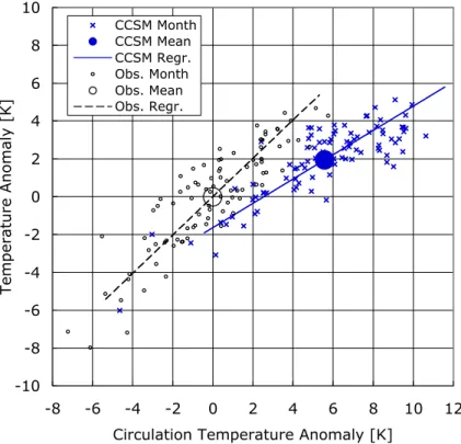
The analysis procedure described by Eqs. (2)–(5) is illustrated in Fig. 8, which shows 20

scatter plots, means and regression lines of simulated and observed temperature anomalies against circulation temperature anomalies.

Next we analyse the performance of 10 models. In Fig. 9a we show the monthly correlations. In winter all models show high correlations, similar to the observed corre-lations. In summer some models show markedly lower than observed correcorre-lations. In 25

(12)

ACPD

Full Screen / Esc

variations in a similar manner as the real climate. In Fig. 9b, we show the slope of the regression lines. These are reasonably close to unity. There seems to be a tendency that models with a westerly circulation bias simulate lower slopes than models with an easterly bias. This is consistent with the idea that a westerly circulation bias leads to a more maritime climate, which is less variable, while an easterly bias produces a more 5

continental and more variable climate. Thus a mean bias in the circulation may have a profound influence on the variability of the monthly mean temperatures.

Next we look at biases in the mean temperature. In Fig. 10 we show the total tem-perature bias in the 20th-century model simulations, the temtem-perature bias attributable to circulation biases and the residual temperature bias, which is obtained by subtract-10

ing the circulation induced bias from the total bias. We see a wide range in biases. The circulation induced biases are largest for GISSer and CCSM3. This is understand-able, because these models have the strongest circulation biases. CCC3.1 has the largest residual bias in particular in March–April. This pronounced cold bias can be partly explained by a pronounced cold bias in the Northern Hemisphere temperatures 15

simulated by this model. Also GFDL2.1 has a cold Northern Hemisphere bias. These results show that an analysis of regional circulation statistics should be an integral part of the validation of regional model performance, since circulation induced biases can be of the same order as other biases. A much more detailed analysis would be needed to understand all the biases, but this falls outside the scope of this paper.

20

3.4. Relations between circulation variations and precipitation variations

The analysis for precipitation is very similar to that for temperature. Circulation Precip-itation Anomalies were defined as:

CP rA= B_S∆G_S + B_W∆G_W + B_V∆G_V + M . (6)

This model performs quit well, with correlations around 0.7 for summer months and 25

(13)

ACPD

Full Screen / Esc

explained variance for all months, but the geostrophic vorticity∆G_V is almost as impor-tant. We found no memory effects.

In Fig. 11a, we show the correlations between precipitation and circulation for the observations and for the model simulations. We see that, in general, the models have higher than observed correlations. Only GISSer shows low correlations in summer. 5

Figure 11b shows the slope of the precipitation regression lines. In general this simu-lated slope is weaker than observed. This is partly caused by the higher than observed variability in the Geostrophic Vorticity that is simulated by the models (see Fig. 6b).

In Fig. 12 we show the precipitation biases for the 20th century simulations. These biases are given as a percentage of the monthly mean observed precipitation. We see 10

that the biases are large. Noteworthy are the large circulation bias for CCSM3 in winter and the wet bias for GFDL2.1 and HadCM3 in summer. GISSer has a dry bias in many months. Again it is apparent that for a region like West-Central Europe it is useful to consider circulation statistics when validating simulated precipitation.

4. Climate change in West-Central Europe from the 20th century to 2071–2100 15

4.1. Mean changes

In the previous sections we have seen that only models with reasonable circulation statistics are credible enough for using them to analyse climate change. For HadGEM no scenario simulations were available at the time this analysis was made. This leaves 7 credible models for the analysis of climate change in West-Central Europe. For 20

6 models A2 scenario simulations were available, while for MIROChi an A1B emission scenario was used.

In Fig. 13 we show the mean change in geostrophic flow indices from the 20th cen-tury to the scenario period 2071–2100. Although the models differ significantly in the extent of the simulated circulation changes, there is a general pattern in the changes. 25

(14)

ACPD

Full Screen / Esc

In late summer (July–September) there is a tendency towards more north-easterly and more anticyclonic flow. These simulated circulation changes resemble the trends in the atmospheric circulation that have been observed in the later part of the 20th century (Van Oldenborgh and van Ulden, 2003; Osborn, 2004). It is still unclear if this is a robust aspect of climate change due to greenhouse gas forcing.

5

Figure 14 shows total temperature changes, changes due to circulation changes and residual changes. Total changes (Fig. 14a) are highest in late summer (J, A, S), while winter months show a secondary maximum. This annual cycle in the tempera-ture changes seems to be at least partly due to circulation changes, as is shown in Fig. 14b. August shows the larges range in circulation induced temperature changes: 10

from almost no change for MIROChi and MRI2.3.2 to more than 3 K for GFDL2.1. The residual temperature changes in Fig. 14c also show a large range, but the changes are more evenly distributed over the year. In this figure the differences re-flect, amongst other factors, the differences in global climate sensitivity between the models.

15

These results suggest that it may be feasible to construct climate change scenarios by decomposing temperature changes into a part that scales with changes in global mean temperature and a part that is related to changes in circulation. This idea has been explored by Van Oldenburgh and van Ulden (2003) for the observed climate in the Netherlands. Such a decomposition may be even more useful in the simulations of 20

precipitation changes, which are shown in Fig. 15.

In Fig. 15a we see a very pronounced annual cycle in simulated precipitation changes for 5 of the 7 models. In the circulation induced precipitation changes this feature is even present for all models, allthough the amplitude of this annual cycle varies considerable between models. After removal of the circulation signal, a much 25

more transparant residual signal results. For most months a modest increase in pre-cipitation is shown. This increase is probably related to changes in the partitioning of the radiative flux convergence at the earth surface over the atmospheric latent and sensible heat fluxes and the heat flux into soil and water. This partitioning depends on

(15)

ACPD

Full Screen / Esc

the temperature, at least over surfaces with sufficient moisture supply (Priestley and Taylor, 1972; Holtslag and van Ulden, 1983). All other things being equal, this theory predicts an increase in evaporation of about 2% per degree warming. The models that are analysed here produce a warming of about 3–4 K. Thus we would expect an increase in precipitation of about 7% in the absence of circulation changes. This is 5

roughly consistent with the results shown in Fig. 15c.

In late summer (J, A, S) soil moisture depletion may play an important role in the hydrological budget. If the soil dries out the evaporation is reduced and simple relations between temperature and precipitation break down. If a model is insufficiently capable of conserving winter precipitation till late summer, the model may have a dry bias which 10

becomes only apparent in late summer (Van den Hurk et al., 2005; Lenderink et al., 2005; Van Ulden et al., 2005). While severe summer drying does occur occasionally in West-Central Europe (for example in 2003), it may happen far more often in some models, while it does not in other models. This may explain the wide range of model results for late summer. We will return to this issue in the next section where we look 15

at specific distributions for the 6 models which used an A2 scenario. 4.2. Changes in distributions

In this section we use scatter plots of the type introduced in Fig. 8, for illustrating and discussing changes in distributions for 6 models. Each figure gives the regression line and the mean for the observations, while scatter plots, regression and means are 20

given for the simulated periods 1971–2000 and 2071–2100. Because these periods cover only 30 y, we combine monthly values of December, January and February into one ensemble of 90 months to represent winter months distributions. In order to rep-resent late summer distributions we combine July, August and September. We first discuss temperature and precipitation changes for winter months, which are shown in 25

the Figs. 16 and 17.

In Fig. 16 we see that the slope of the regression line for temperature decreases in the scenario simulations. At higher temperatures the sensitivity of the temperature

(16)

ACPD

Full Screen / Esc

to circulation variations is reduced. This is caused by two factors. In the first place warmer temperatures reduce the impact of cold snow feed backs. In the second place the simulated shift to warmer circulations leads to a lower frequency of months with a cold snow feedback. Therefore, cold extremes are highly sensitive to changes in the atmospheric circulation.

5

Figure 17 gives the simulations for precipitation. Here we see a general increase in the variablity in the scenario simulations. A certain increase in the slopes is to be expected, because a temperature increase will enhance all precipitation by a similar percentage, which automatically leads to a steeper slope.

In Fig. 18 we show the temperature simulations for late summer. We see that the 10

models differ greatly in these summer simulations. MRI2.3.2 and CCC3.1 show hardly any change in the slope of the regression line. ECHAM5 and MIROChi show a mod-est increase in variability. HadCM3 and especially GFDL2.1 show a very pronounced increase in the slope of the regression line. For an interpretation of these results it is useful to look at the precipitation simulations as well. Figure 19 shows that HadCM3 15

and especially GFDL2.1 show the most pronounced changes towards dry circulations. This is primarily caused by an increase in the frequency of easterly continental flow. Therefore, the strong temperature response of these two models can be understood as follows. Enhanced frequencies of dry flows from the continent lead to an enhanced soil moisture depletion, to a reduction in evaporation and an enhancement of the sen-20

sible heat flux which produces strong warming. These interactions have a pronounced impact on the scaling of precipitation with temperature. While this scaling works well for westerly flow from the Atlantic Ocean, it breaks down for easterly flow in late sum-mer. For easterly flow in late summer the reduction of evaporation may reverse the precipitation-temperature relation, as has been shown by Lenderink et al. (2005) in a 25

detailed analysis of the variability of summer time temperatures. It is even possible that the atmospheric circulation in summer is affected by differential heating due to soil moisture depletion (Van Ulden et al., 2005).

(17)

ACPD

Full Screen / Esc

of circulation changes, soil moisture depletion and possible dynamical feedbacks to the resulting heating. The coupled climate models differ wildly in the simulation of these factors. Apparently, the future summer climate is hard to predict.

5. Discussion

Many coupled climate models are able to simulate the long-term mean of monthly 5

global patterns of the sea level pressure. Unfortunately, this is not the case for northern midlatitudes and for Europe. An important result of the present analysis is that bias patterns in sea level pressure fields simulated by global coupled models have very large scales of thousands of kilometers. This has consequences for the practice of regional climate modeling, which relies on boundary conditions produced by global 10

models. If such models have large-scale errors in their simulations, it is likely that these errors are to a great extent imported by the nested regional models.

We analysed a subset of models that performed well for Europe in more detail. For these models the statistics of geostrophic flow indices were compared with observa-tions. We found that models differed significantly in their simulation of the frequency 15

distribution of the west component of the geostrophic wind. Apparently, models have difficulties in getting the frequency of blocking situations correct. This deficiency and other errors in simulated circulations have an important impact on simulated temper-atures and precipitation. In particular, distributions of monthly mean temperature and precipitation are quite sensitive to biases and changes in the distribution of geostrophic 20

flow indices.

Many models show changes in the simulated atmospheric circulations between the control runs and the scenario run. Simulations for winter months show in general a shift towards warmer and wetter circulations (stronger westerlies). Temperature vari-ability is reduced, while the varivari-ability in precipitation increases in winter. Simulations 25

for summer months show a shift towards warmer and drier circulations (stronger east-erlies). Temperature and precipitation variability increase in future summers. The net

(18)

ACPD

Full Screen / Esc

change in mean summer precipitation is unclear. Some models give a net precipitation increase, while other models simulate drier summers.

The simple model that we have used to describe relations between circulations on the one hand and temperature and precipitation on the other hand is useful to de-scribe the climate in West-Central Europe for most months of the year at the present 5

levels of uncertainty. In late summer, non-linear feedbacks involving soil moisture ren-der its utility more limited. Still it serves to demonstrate that biases and changes in the atmospheric circulation deserve far more attention in model validation and in the development of climate change scenarios than these issues have received in the past.

Acknowledgements. We acknowledge the international modeling groups for providing their

10

data for analysis, the Program for Climate Model Diagnosis and Intercomparison (PCMDI) for collecting and archiving the model data, the JSC/CLIVAR Working Group on Coupled Mod-elling (WGCM) and their Coupled Model Intercomparison Project (CMIP) and Climate Simula-tion Panel for organizing the model data analysis activity, and the IPCC WG1 TSU for technical support. The IPCC Data Archive at Lawrence Livermore National Laboratory is supported by

15

the Office of Science, U.S. Department of Energy.

References

Achuta Rao, K., Covey, C., Doutriaux, C., Fionino, M., Gleckler, P., Philips, T., Sperber, K., and Taylor, K.: An Appraisal of Coupled Climate Model Simulations, edited by: Bader, D., University of California, Lawrence Livermore National Laboratory, UCRL-TR-202550, 197,

20

2004.

Bromwich, D. H. and Fogt, R. L.: Strong trends in the skill of the ERA-40 and NCEP-NCAR reanalysies in the high and midlatitudes of the Southern Hemisphere, J. Climate, 17, 4603– 4619, 2004.

D’Andrea, F., Tibaldi, S., Blackburn, M., Boer, G., D ´equ ´e, M., Dugas, B., Ferranti, L., Hunt, B.,

25

Kitho, A., Randall, D., Roeckner, E., Rowell, D., Straus, D., Sato, N., van den Dool, H. and Williamson, D.: Northern Hemisphere atmospheric blocking as simulated by 15 atmospheric general circulation models in the period 1979–1988, Clim. Dyn., 14, 385–407, 1998.

(19)

ACPD

Full Screen / Esc

Print Version Interactive Discussion Delworth, T. L., Broccoli, A. J., Rosati, A., Stouffer, R. J., Balaji, V., Beesley, J. A., Cooke,W. F.,

Dixon, K. W., Dunne, J., Dunne, K. A., Durachta, J. W., Findell, K. L., Ginoux, P., Gnanade-sikan, A., Gordon, C. T., Griffies, S. M., Gudgel, R., Harrison, M. J., Held, I. M., Hemler, R. S., Horowitz, L. W., Klein, S. A., Knutson, T. R., Kushner, P. J., Langenhorst, A. R., Lee, H. C., Lin, S. J., Lu, J., Malyshev, S. L., Milly, P. C. D., Ramaswamy, V., Russell, J., Schwarzkopf,

5

M. D., Shevliakova, E., Sirutis, J. J., Spelman, M. J., Stern, W. F., Winton, M., Wittenberg, A. T., Wyman, B., Zeng, F., and Zhang, R.: GFDL’s CM2 global coupled climate models – Part 1: formulation and simulation characteristics, J. Climate, accepted, 2005.

Gordon, C., Cooper, C., Senior, C. A., Banks, H., Gregory, J. M., Johns, T. C., J. F. B. Mitchell, J. F. B., and R. Wood, R. A.: The simulation of SST, sea ice extents and ocean heat transport

10

in a version of the Hadley Centre coupled model without flux adjustments, Climate Dyn., 16, 147–168, 2000.

Gordon, H. B., Rotstayn, L. D., McGregor, J. L., Dix, M. R., Kowalczyk, E. A., O’Farrell, S. P., Waterman, L. J., Hirst, A. C., Wilson, S. G., Collier, M. A., Watterson, I. G., and Elliott, T. I.: The CSIRO Mk3 climate system model, Technical Report 60, CSIRO Atmospheric Research,

15

Aspendale,www.dar.csiro.au/publications/gordon 2002a.pdf, 2002.

Holtslag, A. A. M., and van Ulden, A. P.: A simple scheme for daytime estimates of the surface fluxes from routine weather data, J. Climate Appl. Meteor, 22, 517–529, 1983.

IPCC 2001: Climate Change 2001: The Scientific Basis, Contribution of Working Group I to the Third Assessment Report of the Intergovernmental Panel on Climate Change, Cambrige

20

University Press, 881, 2001.

Johns, T., Durman, C., Banks, H., Roberts, M., McLaren, A., Ridley, J., Senior, C., Williams, K., Jones, A., Keen, A., Rickard, G., Cusack, S., Joshi, M., Ringer, M., Dong, B., Spencer, H., Hill, R., Gregory, J., Pardaens, A., Lowe, J., Bodas-Salcedo, A., Start, S., and Searl, Y.: HadGEM1 model description and analysis of preliminary experiments for the IPCC Fourth

25

Assessment Report, Technical Report 55, U.K. Met Office, Exeter, U.K. ,www.metoffice.gov.

uk/research/hadleycentre/pubs/HCTN/index.html, 2004.

Jones, P. D., Davies, T. D., Lister, D. H., Slonosky, V., Jonsson, T., Barring, L., Jonsson, P., Maheras, P, Kolyva-Machera, F., Barriendos, M., Martin-Vide, J., Rodriquez, R., Alcoforado, M. J., Wanner, H., Pfister, C., Luterbacher, J., Rickli, R., Schuepbach, E., Kaas, E., Schmith,

30

T., Jacobeit, J., and Beck, C.: Monthly mean pressure reconstructions for Europe for the 1780–1995 period, Int. J. Climatol., 19, 347–364, 1999.

(20)

ACPD

Full Screen / Esc

Print Version Interactive Discussion the 21st century, Boreal Env. Res., 9, 127–152, 2004.

K-1 Model Developers: K-1 coupled model (MIROC) description, Technical Report 1, Center for

Climate System Research, University of Tokyo,http://www.ccsr.u-tokyo.ac.jp/kyosei/hasumi/

MIROC/tech-repo.pdf, 2004.

Kim, S.-J., Flato, G. M., de Boer, G. J., and McFarlane, N. A.: A coupled climate model

simula-5

tion of the last glacial maximum, part 1: transient multi-decadal response, Climate Dyn., 19, 515–537, 2002.

K ˚allberg, P., Simmons, A., Uppala S., and Fuentes, M.: The ERA-40 Archive, ERA-40 Project Report Series No. 17, ECMWF, Sept., 2004.

Lucarini, L. and Russell, G. L.: Comparison of mean climate trends in the northern hemisphere

10

between National Centers for Environmental Prediction and two atmosphere-ocean model forced runs, J. Geophys. Res., 107(D15), 4269, 2002.

Marti, O., Braconnot, P., Bellier, J., Benshila, R., Bony, S., Brockmann, P., Cadule, P., Caubel, A., Denvil, S., Dufresne, J.-L., Fairhead, L., Filiberti, M.-A., Foujols, M.-A., Fichefet, T., Friedlingstein, P., Gosse, H., Grandpeix, J.-Y., Hourdin, F., Krinner, G., Lvy, C., Madec, G.,

15

Musat, I., de Noblet, N., Polcher, J., and Talandier, C.: The new IPSL climate system model: IPSL-CM4, Technical Report, Institut Pierre Simon Laplace des Sciences de l’Environnement Global, IPSL, Case 101, 4 place Jussieu, Paris, France, 84, 2005.

New, M., Hulme, M., and Jones, P.: Representing Twentiest-Century Space-Time Climate Vari-ability, Part 1: Development of a 1961–90 Mean Monthly Terrestrial Climatology, J. Climate,

20

12, 829–856, 1999.

New, M., Hulme, M., and Jones, P.: Representing Twentiest-Century Space-Time Climate Vari-ability. Part I1: Development of a 1901–96 Monthly Grids of Terrestrial Surface Climate, J. Climate, 13, 2217–2238, 2000.

Osborn, T. J.: Simulating the winter North Atlantic Oscillation: the roles of internal variability

25

and greenhouse gas forcing, Climate Dyn., 22, 605–623, 2004.

Priestley, C. H. B. and Taylor, R. J.: On the assessment of surface heat flux and evaporation using large-scale parameters, Mon. Weather Rev., 106, 81–92, 1972.

Schmidt, G. A., Ruedy, R., Hansen, J. E., Aleinov, I., Bell, N., Bauer, M., Bauer, S., Cairns, B., Canuto, V., Cheng, Y., Del Genio, A., Faluvegi, G., Friend, A. D., Hall, T. M., Hu, Y.,

30

Kelley, M., Kiang, N. Y., Koch, D., Lacis, A. A., Lerner, J., Lo, K. K., Miller, R. L., Nazarenko, L., Oinas, V., Perlwitz, Ja., Perlwitz, Ju., Rind, D., Romanou, A., Russell, G. L., Sato, Mki., Shindell, D. T., Stone, P. H., Sun, S., Tausnev, N., Thresher, D., and Yao, M.-S.: Present day

(21)

ACPD

Full Screen / Esc

Print Version Interactive Discussion atmospheric simulations using GISS ModelE: Comparison to in-situ, satellite and reanalysis

data, J. Climate, accepted, 2005.

Thorpe, R. P.: The impact of changes in atmospheric and land surface physics on the thermo-haline circulation response to anthropogenic forcing in HadCM3 and HadCM2, Clim. Dyn., 24, 449–456, 2005.

5

Turnpenny, J. R., Crossley, J. F., Hulme ,M., and Osborne, T. J.: Air flow influences on local climate: comparison of a regional climate model with observations over the United Kingdom, Clim. Res., 20, 189–202, 2002.

Van den Hurk, B., Hirschi, M., Lenderink, G., van Meijgaard, E., van Ulden, A. P., Rockel, B., Hagemann, S., Graham, P., Kjellstr ¨om, E., and Jones, R.: Soil control on run-off response to

10

climate change in regional climate model simulations, J. Climate, accepted, 2005.

Van Oldenborgh, G. J., and van Ulden, A. P.: On the relationship between global warming, local warming in the Netherlands and changes in circulation in the 20th century, Int. J. Climatol., 23, 1711–1724, 2003.

Volodin, E. M. and Diansky, N. A.: El-Nino reproduction in coupled general circulation model of

15

atmosphere and ocean, Russian meteorology and hydrology, vol. 12, 5–14, 2004.

Washington, W. M., Weatherly, J. W., Meehl, G. A., Semtner Jr., A. J., Bettge, T. W., Craig, A. P., Strand Jr., W. G., Arblaster, J., Wayland, V. B., James, R., and Zhang, Y.: Parallel climate model (PCM) control and transient simulations, Climate Dyn., 16, 755–774, 2000.

Yu, Y., Zhang, X., and Guo, Y.: Global coupled ocean- atmosphere general circulation models

20

in LASG/IAP, Adv. Atmos. Sci., 21, 444–455, 2004.

Yukimoto, S. and Noda, A.: Improvements of the Meteorological Research Institute Global Ocean-atmosphere Coupled GCM (MRI-CGCM2) and its climate sensitivity, Technical

Re-port 10, NIES, Japan,www.mri-jma.go.jp/Dep/cl/cl4/publications/yukimoto CGER2002.pdf,

2002.

(22)

ACPD

Full Screen / Esc

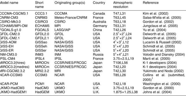
Print Version Interactive Discussion Table 1. Models included in this study.

Model name Short Originating group(s) Country Atmospheric Reference

name resolution

CCCMA-CGCM3.1 CCC3.1 CCCMA Canada T47,L31 Kim et al. (2002) CNRM-CM3 CNRM3 Meteo-France/CNRM France T63,L45 Salas-M’elia et al. (2005) CSIRO-Mk3.0 CSIRO3 CSIRO Australia T63,L18 Gordon et al. (2002) ECHAM5/MPI-OM ECHAM5 MPI Germany T63,L31 Jungclaus et al. (2005) FGOALS-g1.0 FGOALS LASG/IAP China T42,L26 Yu et al. (2004) GFDL-CM2.0 GFDL2.0 GFDL USA 2.5◦×2◦,L24 Delworth et al. (2005) GFDL-CM2.1 GFDL2.1 GFDL USA 2.5◦×2◦,L24 Delworth et al. (2005) GISS-AOM GISSao NASA/GISS USA 4◦×3◦,L12 Lucarini & Russell (2002) GISS-EH GISSeh NASA/GISS USA 5◦×4◦,L20 Schmidt et al. (2005) GISS-ER GISSer NASA/GISS USA 5◦×4◦,L20 Schmidt et al. (2005) INM-CM3.0 INM3 INM Russia 5◦×4◦,L21 Volodin and Diansky (2004) IPSL-CM4 IPSL4 IPSL France 3.75×2.5,L19 Marti et al. (2005)

MIROC3.2(hires) MIROChi CCSR/NIES/FRCGC Japan T106,L56 K-1 developers (2004) MIROC3.2(medres) MIROCm CCSR/NIES/FRCGC Japan T42,L20 K-1 developers (2004) MRI-CGCM2.3.2 MRI2.3.2 MRI Japan T42,L30 Yukimoto and Noda (2002)

NCAR-CCSM3 CCSM3 NCAR USA T85,L26 Collins et al. (submitted,

2005)1

NCAR-PCM PCM1 NCAR USA T42,L18 Washington et al. (2000)

UKMO-HadCM3 HadCM3 UKMO U.K. 3.75×2.5,L19 Gordon et al. (2000) UKMO-HadGEM1 HadGEM UKMO U.K. 1.875×1.25,L38 Johns et al. (2004)

1

– Collins, W. D., Bitz, C. M., Blackmon, M. I., Bonan, G. B., Bretherton, C. S., Carton, J. A., Chang, P., Doney, S. C., Hack, J. J., Henderson, T. B., Kiehl, J. T., Large, W. G., McKenna, D. S., Santer, B. D., and Smith, R. D.: The Community Climate System Model: CCSM3, J. Climate, submitted, 2005.

(23)

ACPD

Full Screen / Esc

Print Version Interactive Discussion Table 2. Quality of simulated mean sea level pressure on global and regional scales.

Globe stde hPa Tropics stde hPa S.Lat. stde hPa N.Lat stde hPa Europe stde hPa Globe expl. fraction Tropics expl. fraction S.Lat. expl. fraction N.Lat. expl. fraction Europe expl. fraction CCC3.1 4.1 1.6 6.1 3.2 1.9 0.83 0.84 0.75 0.51 0.80 CNRM3 7.6 1.5 10.1 3.3 3.4 0.45 0.85 0.31 0.49 0.51 CSIRO3 5.6 1.9 6.0 4.6 2.8 0.69 0.77 0.77 0.31 0.68 ECHAM5 2.7 1.6 3.4 2.5 1.7 0.93 0.84 0.93 0.70 0.83 GFDL2.0 3.9 1.6 4.5 3.9 2.7 0.85 0.85 0.86 0.32 0.59 GFDL2.1 3.0 1.8 3.2 2.9 2.4 0.91 0.81 0.93 0.63 0.75 GISSao 8.9 1.6 13.0 3.6 2.8 0.24 0.83 -0.05 0.47 0.68 GISSeh 8.7 2.6 11.6 4.7 3.9 0.27 0.58 0.18 -0.09 0.16 GISSer 8.1 2.6 10.4 5.4 4.5 0.36 0.60 0.35 -0.34 -0.14 FGOALS 4.5 1.8 5.5 4.2 3.5 0.80 0.80 0.80 0.18 0.43 INM3 4.1 1.8 4.8 4.0 3.6 0.83 0.80 0.85 0.30 0.42 IPSL4 12.6 1.8 19.1 5.5 3.2 -0.56 0.79 -1.36 -0.23 0.53 MIROChi 4.6 1.6 5.2 2.9 1.7 0.79 0.83 0.83 0.68 0.85 MIROCm 4.5 1.9 5.8 3.5 2.6 0.80 0.78 0.78 0.56 0.71 MRI2.3.2 4.3 1.5 5.1 4.3 2.4 0.82 0.86 0.84 0.30 0.75 CCSM3 5.4 1.8 5.2 5.0 5.3 0.71 0.80 0.82 -0.23 -0.60 PCM 6.4 2.8 9.7 3.8 4.8 0.60 0.50 0.43 0.34 -0.08 HadCM3 4.6 2.1 4.7 4.4 2.5 0.79 0.72 0.86 0.23 0.69 HadGEM 4.0 2.1 5.3 2.8 1.9 0.84 0.73 0.82 0.64 0.83

(24)

ACPD

Full Screen / Esc

Print Version Interactive Discussion Europe 0 1 2 3 4 5 6 7 8 0 1 2 3 4 5 6 7 8 9 10 11 12 Month stde [hPa] MIROChi ECHAM5 HadGEM CCC3.1 GFDL2.1 MRI2.3.2 HadCM3 MIROCm GFDL2.0 CSIRO3 GISSao IPSL4 CNRM3 FGOALS INM3 GISSeh GISSer PCM CCSM3 std Obs. Nat. Var. ERA-40

Figure 1. Spatial standard deviation of the difference between simulated sea level pressure fields and the longterm mean observed pressure field. Std Obs. is the spatial standard deviation of the observed field. Nat. Var. is the mean spatial standard deviation of the differences between 30 year averaged observed fields and the longterm mean observed field. ERA-40 is the spatial standard deviation of ERA-40 averaged over the last 30 year, relative to the long-term mean observed field.

Fig. 1. Spatial standard deviation of the difference between simulated sea level pressure fields and the longterm mean observed pressure field. Std Obs. is the spatial standard deviation of the observed field. Nat. Var. is the mean spatial standard deviation of the differences between 30 year averaged observed fields and the longterm mean observed field. ERA-40 is the spatial standard deviation of ERA-40 averaged over the last 30 year, relative to the long-term mean observed field.

(25)

ACPD

Full Screen / Esc

Print Version Interactive Discussion Figure 2. European domains. The full picture gives the European test domain for pressure patterns

used in section 2. It depicts the annual mean observed sea level pressure field for the 20th century. The interval width is 2hPa, except for the grey region, which represents the interval 1012-1016 hPa. In the southwest corner the Azores High is visible, while in the northwest the Iceland Low can be seen. The large rectangle is the region West-Central Europe for which the geostrophic flow indices are computed. The small rectangle is the test region for temperature and precipitation.

Fig. 2. European domains. The full picture gives the European test domain for pressure pat-terns used in Sect. 2. It depicts the annual mean observed sea level pressure field for the 20th century. The interval width is 2 hPa, except for the grey region, which represents the interval 1012–1016 hPa. In the southwest corner the Azores High is visible, while in the northwest the Iceland Low can be seen. The large rectangle is the region West–Central Europe for which the geostrophic flow indices are computed. The small rectangle is the test region for temperature and precipitation.

(26)

ACPD

Full Screen / Esc

Print Version Interactive Discussion Mean G-west -4 -2 0 2 4 6 8 10 12 0 1 2 3 4 5 6 7 8 9 10 11 12 Month m/s MIROChi ECHAM5 HadGEM CCC3.1 GFDL2.1 MRI2.3.2 MIROCm HadCM3 GISSer CCSM3 Observed

Figure 3a. Mean west component of the geostrophic wind for the 20th century.

Standard Deviation G-west

0 1 2 3 4 5 0 1 2 3 4 5 6 7 8 9 10 11 12 Month m/s MIROChi ECHAM5 HadGEM CCC3.1 GFDL2.1 MRI2.3.2 MIROCm HadCM3 GISSer CCSM3 Observed

Figure 3b. Standard deviation of west component of geostrophic wind.

(a) Mean G-west -4 -2 0 2 4 6 8 10 12 0 1 2 3 4 5 6 7 8 9 10 11 12 Month m/s MIROChi ECHAM5 HadGEM CCC3.1 GFDL2.1 MRI2.3.2 MIROCm HadCM3 GISSer CCSM3 Observed

Figure 3a. Mean west component of the geostrophic wind for the 20th century.

Standard Deviation G-west

0 1 2 3 4 5 0 1 2 3 4 5 6 7 8 9 10 11 12 Month m/s MIROChi ECHAM5 HadGEM CCC3.1 GFDL2.1 MRI2.3.2 MIROCm HadCM3 GISSer CCSM3 Observed

Figure 3b. Standard deviation of west component of geostrophic wind.

(b)

Fig. 3. (a) Mean west component of the geostrophic wind for the 20th century. (b) Standard deviation of west component of geostrophic wind.

(27)

ACPD

Full Screen / Esc

Cumulative Frequency Distribution for Januari

0 10 20 30 40 50 60 70 80 90 100 -6 -4 -2 0 2 4 6 8 10 12 14 16 18 G-West [m/s] Quantile [%] Observed MIROChi ECHAM5 HadGEM CCC3.1 GFDL2.1 MRI2.3.2 MIROCm HadCM3 GISSer CCSM3 G-west=0

Figure 4a. Cumulative frequency distribution of the west component of the geostrophic wind for January in the 20th century.

Cumulative Frequency Distribution for July

0 10 20 30 40 50 60 70 80 90 100 -6 -5 -4 -3 -2 -1 0 1 2 3 4 5 6 7 G-West [m/s] Quantile [%] Observed MIROChi ECHAM5 HadGEM CCC3.1 GFDL2.1 MRI2.3.2 MIROCm HadCM3 GISSer CCSM3 G-west=0

Figure 4b. As figure 3a, but fot July.

(a)

0 10 20 30 40 50 60 70 80 90 100 -6 -4 -2 0 2 4 6 8 10 12 14 16 18 G-West [m/s] Quantile [%] Observed MIROChi ECHAM5 HadGEM CCC3.1 GFDL2.1 MRI2.3.2 MIROCm HadCM3 GISSer CCSM3 G-west=0

Figure 4a. Cumulative frequency distribution of the west component of the geostrophic wind for January in the 20th century.

0 10 20 30 40 50 60 70 80 90 100 -6 -5 -4 -3 -2 -1 0 1 2 3 4 5 6 7 G-West [m/s] Quantile [%] Observed MIROChi ECHAM5 HadGEM CCC3.1 GFDL2.1 MRI2.3.2 MIROCm HadCM3 GISSer CCSM3 G-west=0

Figure 4b. As figure 3a, but fot July.

(b)

Fig. 4. (a) Cumulative frequency distribution of the west component of the geostrophic wind for January in the 20th century.(b) As Fig. 4a, but for July.

(28)

ACPD

Full Screen / Esc

Print Version Interactive Discussion Mean G-south -4 -2 0 2 4 0 1 2 3 4 5 6 7 8 9 10 11 12 Month m/s MIROChi ECHAM5 HadGEM CCC3.1 GFDL2.1 MRI2.3.2 MIROCm HadCM3 GISSer CCSM3 Observed

Figure 5a. Mean south component of the geostrophic wind for the 20th century.

Standard Deviation G-south

0 1 2 3 0 1 2 3 4 5 6 7 8 9 10 11 12 Month m/s MIROChi ECHAM5 HadGEM CCC3.1 GFDL2.1 MRI2.3.2 MIROCm HadCM3 GISSer CCSM3 Observed

Figure 5b. Standard deviation of south component of geostrophic wind.

(a) Mean G-south -4 -2 0 2 4 0 1 2 3 4 5 6 7 8 9 10 11 12 Month m/s MIROChi ECHAM5 HadGEM CCC3.1 GFDL2.1 MRI2.3.2 MIROCm HadCM3 GISSer CCSM3 Observed

Figure 5a. Mean south component of the geostrophic wind for the 20th century.

Standard Deviation G-south

0 1 2 3 0 1 2 3 4 5 6 7 8 9 10 11 12 Month m/s MIROChi ECHAM5 HadGEM CCC3.1 GFDL2.1 MRI2.3.2 MIROCm HadCM3 GISSer CCSM3 Observed

Figure 5b. Standard deviation of south component of geostrophic wind. (b)

Fig. 5. (a) Mean south component of the geostrophic wind for the 20th century. (b) Standard deviation of south component of geostrophic wind.

(29)

ACPD

Full Screen / Esc

Mean Geostrophic Vorticity

-3 -2 -1 0 1 2 0 1 2 3 4 5 6 7 8 9 10 11 12 Month hPa MIROChi ECHAM5 HadGEM CCC3.1 GFDL2.1 MRI2.3.2 MIROCm HadCM3 GISSer CCSM3 Observed

Figure 6a. Mean geostrophic vorticity for the 20th century.

Standard Deviation Geostrophic Vorticity

0 0.5 1 1.5 2 0 1 2 3 4 5 6 7 8 9 10 11 12 Month hPa MIROChi ECHAM5 HadGEM CCC3.1 GFDL2.1 MRI2.3.2 MIROCm HadCM3 GISSer CCSM3 Observed

Figure 6b. Standard deviation of geostrophic vorticity for the 20th century. (a)

Mean Geostrophic Vorticity

-3 -2 -1 0 1 2 0 1 2 3 4 5 6 7 8 9 10 11 12 Month hPa MIROChi ECHAM5 HadGEM CCC3.1 GFDL2.1 MRI2.3.2 MIROCm HadCM3 GISSer CCSM3 Observed

Figure 6a. Mean geostrophic vorticity for the 20th century.

Standard Deviation Geostrophic Vorticity

0 0.5 1 1.5 2 0 1 2 3 4 5 6 7 8 9 10 11 12 Month hPa MIROChi ECHAM5 HadGEM CCC3.1 GFDL2.1 MRI2.3.2 MIROCm HadCM3 GISSer CCSM3 Observed

Figure 6b. Standard deviation of geostrophic vorticity for the 20th century.

(b)

Fig. 6. (a) Mean geostrophic vorticity for the 20th century. (b) Standard deviation of geostrophic vorticity for the 20th century.

(30)

ACPD

Full Screen / Esc

0 10 20 30 40 50 60 70 80 90 100 -5 -4 -3 -2 -1 0 1 2 3 4 Geostrophic Vorticity [hPa]

Quantile [%] Observed MIROChi ECHAM5 HadGEM CCC3.1 GFDL2.1 MRI2.3.2 MIROCm HadCM3 GISSer CCSM3 GV=0

Figure 7a. Cumulative frequency distribution of the geostrophic vorticity in the 20th century for January.

0 10 20 30 40 50 60 70 80 90 100 -3 -2 -1 0 1 2 Geostrophic Vorticity [hPa]

Figure 7b. Cumulative frequency distribution of the geostrophic vorticity in the 20th century for July. (a)

Figure 7b. Cumulative frequency distribution of the geostrophic vorticity in the 20th century for July. (b)

Fig. 7. (a) Cumulative frequency distribution of the geostrophic vorticity in the 20th century for January. (b) Cumulative frequency distribution of the geostrophic vorticity in the 20th century for July.

(31)

ACPD

Full Screen / Esc

Print Version Interactive Discussion -10 -8 -6 -4 -2 0 2 4 6 8 10 -8 -6 -4 -2 0 2 4 6 8 10 12

Circulation Temperature Anomaly [K]

Temperature Anomaly [K] CCSM Month CCSM Mean CCSM Regr. Obs. Month Obs. Mean Obs. Regr.

Figure 8. Scatter plots of observed and simulated (CCSM3.2) July temperature anomalies (TA) against circulation temperature anomalies (CTA) for the 20th century. Shown are monthly anomalies, 20th century mean anomalies and regression lines. The length of the regression lines is 4 standard deviations for both axes. The correlations between TA and CTA are 0.87 for the observations and 0.84 for the model simulations. The model simulations have a warm temperature bias of 1.9k and a warm circulation temperature bias of 5.6K. The slope of the regression line is 0.64. This produces a temperature bias due to the circulation bias of 3.6K. This indicates that the model would have shown a negative residual temperature bias of –1.7K, if it had simulated no mean circulation bias.

Fig. 8. Scatter plots of observed and simulated (CCSM3.2) July temperature anomalies (TA) against circulation temperature anomalies (CTA) for the 20th century. Shown are monthly anomalies, 20th century mean anomalies and regression lines. The length of the regression lines is 4 standard deviations for both axes. The correlations between TA and CTA are 0.87 for the observations and 0.84 for the model simulations. The model simulations have a warm temperature bias of 1.9 K and a warm circulation temperature bias of 5.6 K. The slope of the regression line is 0.64. This produces a temperature bias due to the circulation bias of 3.6 K. This indicates that the model would have shown a negative residual temperature bias of –1.7 K, if it had simulated no mean circulation bias.

(32)

ACPD

Full Screen / Esc

Print Version Interactive Discussion TA - CTA Correlation 0 0.2 0.4 0.6 0.8 1 0 1 2 3 4 5 6 7 8 9 10 11 12 Month r MIROChi ECHAM5 HadGEM CCC3.1 GFDL2.1 MRI MIROCm HadCM3 GISSer CCSM3 Observed

Figure 9a. TA-CTA correlations for the 20th century.

Slope of Temperature Regression Line

0 0.5 1 1.5 2 2.5 0 1 2 3 4 5 6 7 8 9 10 11 12 Month stdTA/stdCTA MIROChi ECHAM5 HadGEM CCC3.1 GFDL2.1 MRI MIROCm HadCM3 GISSer CCSM3 Observed

Figure 9b. Slope ST=ΣTA/ΣCTA

(a) TA - CTA Correlation 0 0.2 0.4 0.6 0.8 1 0 1 2 3 4 5 6 7 8 9 10 11 12 Month r MIROChi ECHAM5 HadGEM CCC3.1 GFDL2.1 MRI MIROCm HadCM3 GISSer CCSM3 Observed

Figure 9a. TA-CTA correlations for the 20th century.

Slope of Temperature Regression Line

0 0.5 1 1.5 2 2.5 0 1 2 3 4 5 6 7 8 9 10 11 12 Month stdTA/stdCTA MIROChi ECHAM5 HadGEM CCC3.1 GFDL2.1 MRI MIROCm HadCM3 GISSer CCSM3 Observed

Figure 9b. Slope ST=ΣTA/ΣCTA

(b)

(33)

ACPD

Full Screen / Esc

EGU

Figure 7b. Cumulative frequency distribution of the geostrophic vorticity in the 20th century for July. (a)

Figure 7b. Cumulative frequency distribution of the geostrophic vorticity in the 20th century for July. (b)

Quantile [%] Observed MIROChi ECHAM5 HadGEM CCC3.1 GFDL2.1 MRI2.3.2 MIROCm HadCM3 GISSer CCSM3 GV=0 (c)

Fig. 10. Temperature bias for 20th century. (a) Total, (b) Circulation, (c) Residual.

(34)

ACPD

Full Screen / Esc

Print Version Interactive Discussion Pr - CPrA Correlation 0 0.2 0.4 0.6 0.8 1 0 1 2 3 4 5 6 7 8 9 10 11 12 Month r MirocHi ECHAM5 HadGEM CCC3.1 gfdl2.1 MRI MIROCm HadCM3 GISSer CCSM3 Observed

Figure 11a. Correlations between precipitation and circulation for the 20th century.

Slope of Precipitation Regression Line

0 0.5 1 1.5 2 2.5 0 1 2 3 4 5 6 7 8 9 10 11 12 Month stdPrA/stdCPrA MirocHi ECHAM5 HadGEM CCC3.1 gfdl2.1 MRI MIROCm HadCM3 GISSer CCSM3 Observed

Figure 11b. Slope: SPr = ΣPr/ΣCPrA for the 20th century.

(a) Pr - CPrA Correlation 0 0.2 0.4 0.6 0.8 1 0 1 2 3 4 5 6 7 8 9 10 11 12 Month r MirocHi ECHAM5 HadGEM CCC3.1 gfdl2.1 MRI MIROCm HadCM3 GISSer CCSM3 Observed

Figure 11a. Correlations between precipitation and circulation for the 20th century.

Slope of Precipitation Regression Line

0 0.5 1 1.5 2 2.5 0 1 2 3 4 5 6 7 8 9 10 11 12 Month stdPrA/stdCPrA MirocHi ECHAM5 HadGEM CCC3.1 gfdl2.1 MRI MIROCm HadCM3 GISSer CCSM3 Observed

Figure 11b. Slope: SPr = ΣPr/ΣCPrA for the 20th century.

(b)

Fig. 11. (a) Correlations between precipitation and circulation for the 20th century. (b) Slope: S_Pr=Σ_Pr/Σ_CPrAfor the 20th century.