Bremsstrahlung and K alpha fluorescence
measurements for inferring conversion
efficiencies into fast ignition relevant hot electrons
The MIT Faculty has made this article openly available.
Please share
how this access benefits you. Your story matters.
Citation
Chen, C. D. et al. “Bremsstrahlung and K alpha fluorescence
measurements for inferring conversion efficiencies into fast ignition
relevant hot electrons.” Physics of Plasmas 16.8 (2009): 082705-10.
© 2009 American Institute of Physics
As Published
http://dx.doi.org/10.1063/1.3183693
Publisher
American Institute of Physics
Version
Final published version
Citable link
http://hdl.handle.net/1721.1/52297
Terms of Use
Article is made available in accordance with the publisher's
policy and may be subject to US copyright law. Please refer to the
publisher's site for terms of use.
Bremsstrahlung and K
␣
fluorescence measurements for inferring
conversion efficiencies into fast ignition relevant hot electrons
C. D. Chen,1P. K. Patel,2D. S. Hey,2A. J. Mackinnon,2M. H. Key,2K. U. Akli,3
T. Bartal,4F. N. Beg,4S. Chawla,4H. Chen,2R. R. Freeman,5D. P. Higginson,4A. Link,5 T. Y. Ma,2,4A. G. MacPhee,2R. B. Stephens,3L. D. Van Woerkom,5B. Westover,4 and M. Porkolab1
1Plasma Science Fusion Center, Massachusetts Institute of Technology, Cambridge,
Massachusetts 02139, USA
2Lawrence Livermore National Laboratory, Livermore, California 94550, USA 3General Atomics, San Diego, California 92121, USA
4Department of Mechanical and Aerospace Engineering, University of California-San Diego, La Jolla,
California 92093, USA
5
College of Mathematical and Physical Sciences, The Ohio State University, Columbus, Ohio 43210, USA
共Received 3 April 2009; accepted 29 June 2009; published online 19 August 2009兲
The Bremsstrahlung and K-shell emission from 1⫻1⫻1 mm3 planar targets irradiated by a short-pulse 3⫻1018– 8⫻1019 W/cm2 laser were measured. The Bremsstrahlung was measured using a filter stack spectrometer with spectral discrimination up to 500 keV. K-shell emission was measured using a single photon counting charge coupled device. From Monte Carlo modeling of the target emission, conversion efficiencies into 1–3 MeV electrons of 3%–12%, representing 20%– 40% total conversion efficiencies, were inferred for intensities up to 8⫻1019 W/cm2. Comparisons to scaling laws using synthetic energy spectra generated from the intensity distribution of the focal spot imply slope temperatures less than the ponderomotive potential of the laser. Resistive transport effects may result in potentials of a few hundred kV in the first few tens of microns in the target. This would lead to higher total conversion efficiencies than inferred from Monte Carlo modeling but lower conversion efficiencies into 1–3 MeV electrons. © 2009 American Institute of Physics. 关DOI:10.1063/1.3183693兴
I. INTRODUCTION
The fast ignition1 concept promises higher gains, lower sensitivity to hydrodynamic instabilities, and reduced driver energy when compared to conventional inertial confinement fusion 共ICF兲. This is achieved using a short-pulse laser to ignite a hot spot in a precompressed, 300 g/cc fusion capsule. The laser interacts with the plasma near the critical density surface, generating hot electrons that propagate into the core to heat the hot spot. In cone-guided fast ignition,2–4a high Z cone keeps a channel open in the blowoff plasma, reducing the distance the electrons have to travel to reach the core. The success of fast ignition is primarily dependent on the coupling of the short-pulse laser energy to the hot spot. This can be broken down into three components: the coupling of the laser into relativistic electrons共L→e−兲, the transport
ef-ficiency of the electrons to the core, which depends on the divergence angle and collimation effects 共trans兲, and the deposition of the electron energy in the hot spot, which is a function of the electron energy spectrum 共deposition兲. Simulations5found that to achieve ignition at 300 g/cc, 18 kJ of energy must be deposited in a 40 m diameter hot spot in 20 ps, requiring laser intensities of 2 – 3⫻1020 W/cm2. For a 40 m diameter hot spot, electrons of 1–3 MeV have the ideal range to couple efficiently, making the conversion effi-ciency to 1–3 MeV electrons a critical parameter for fast ignition. For intensities of 2 – 3⫻1020 W/cm2, scaling of the electron energy with the ponderomotive potential of the laser6gives temperatures of 6–8 MeV, reducing the
deposi-tion efficiency and driving up the driver requirements. Re-cent modeling suggests, however, that the slope temperature may be colder than ponderomotive scaling due to the steep-ening of the density gradient.7–9
Previous measurements of the electron spectrum relied on techniques such as vacuum electron spectrometers,10,11 nuclear activation,12Bremsstrahlung spectrometers,13 buried fluorescent foils,14 and proton emission.15Measurements us-ing electron spectrometers and nuclear activation found that the electron slope temperature scales with the laser intensity in proportion to共I2兲1/2 and is close to the ponderomotive potential of the laser. The energies of escaping electrons are however modified by megavolt potentials and significant modeling is required to accurately infer the source spectrum at 1–3 MeV energies of most interest to fast ignition. Nuclear activation is sensitive to photons above 8 MeV and provide limited information about 1–3 MeV electrons. Other mea-surements using Bremsstrahlung and rear surface proton emission found a共I2兲1/3scaling, usually referred to as Beg scaling.15
Conversion efficiencies have been determined by mea-suring and modeling the K␣ yield in very thin foils with strong refluxing. Myatt et al.16and Nilson et al.17found cou-pling efficiencies of 20%⫾10%, independent of the laser intensity for I = 1017– 1020 W/cm2using a hybrid particle in cell model. This model did not include energy transfer to fast ions, making these measurements lower bounds on the con-version efficiency. Yasuike et al.14 used the fluorescence PHYSICS OF PLASMAS 16, 082705共2009兲
yields from buried layer K␣ emitters in thick nonrefluxing foils to infer both the slope temperature and conversion effi-ciency, estimating conversion efficiencies scaling from 10% to 50%, for I = 1018– 1020 W/cm2from Monte Carlo model-ing. However, the slope temperature inferred using Monte Carlo modeling is sensitive to collective electric and mag-netic field effects, which were not included in the analysis. Davies18 has shown that neglect of the Ohmic potential re-sults in an underestimate of the conversion efficiency.
In this paper we describe measurements of the number of 1–3 MeV electrons using absolute Bremsstrahlung and K-shell fluorescence emission from planar foil targets irradi-ated by a short-pulse laser. From Monte Carlo transport mod-eling, the laser conversion efficiency into fast ignition rel-evant 1–3 MeV electrons is inferred by fitting both the Bremsstrahlung measurements and the fluorescence yield. The sensitivity of the inferred conversion efficiency to the details of the method of analysis is also discussed. The re-sults are compared to scaling laws and modeling estimates commonly used in simulations of fast ignition.
This paper starts with an overview of the experiment and Bremsstrahlung and K-shell diagnostics. It then describes the Monte Carlo simulation of the target and techniques for un-folding the electron spectrum from the simulation. This is followed by comparisons of the data to different scaling laws and summaries of the inferred conversion efficiencies. The paper concludes with a discussion on the role of the assumed electron cone angles and resistive transport effects on the deduction of the conversion efficiencies.
II. EXPERIMENT OVERVIEW
Experiments were performed on the Titan laser at Lawrence Livermore National Laboratory.19 Titan is a 1.06 m laser with a maximum energy of 150 J at 0.7 ps pulse length. Focusing is with an f/3 off-axis parabola. The focal spot at target chamber center was imaged at low power with a 16-bit charge coupled device共CCD兲 camera, which shows a full width at half maximum共FWHM兲 of 7 m and ⬃15% of the laser energy within the FWHM. The prepulse was measured on each shot with a water cell protected fast diode and the preformed plasma was diagnosed with a 20 interferometer. Prepulse levels for the data shown here ranged from 5 to 80 mJ in a 3 ns pedestal before the main pulse with a 1–30 mJ parasitic short pulse 1.4 ns ahead of the main pulse.20From hydrodynamic modeling of the prepulse, preformed plasma scale lengths are estimated at up to 10 m for the critical surface and 50 m for 1/10th critical. The pulse length was measured at 0.7⫾0.3 ps using a sec-ond order autocorrelator.
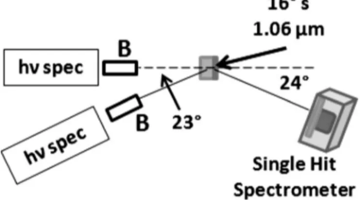
The targets consisted of 1⫻1 mm2 sandwich targets, layered with 10 m Al at the interaction surface, 25 m Cu for a fluor, and a 1 mm Al layer to range out the electrons and prevent multiple passes through the Cu共refluxing兲. They were irradiated at 16° horizontal off normal s-polarization with 5–150 J of laser energy for intensities averaged over the FWHM region共containing 15% of the laser energy兲 from 3 ⫻1018to 8⫻1019 W/cm2. Two filter stack Bremsstrahlung spectrometers21 measured the x-ray emission at rear target
normal共TN兲 and at 23° horizontal to rear TN, about 80 cm from the target. A Spectral Instruments SI-800 CCD operat-ing in soperat-ingle hit mode22 was used to measure the K-shell emission from the buried Cu layer at 24° horizontal to the front TN. A schematic of the setup is shown in Fig.1.
III. BREMSSTRAHLUNG SPECTROMETER DESCRIPTION AND CALIBRATION
The Bremsstrahlung spectrometer consists of a stack of 13 filters from 100 m Al to 4 mm Pb alternating with image plate共IP兲 dosimeters. It is able to differentiate photons up to 500 keV. A magnet was used to eliminate electron contamination共⬍100 MeV兲 and a 5 in. Pb collimator with a 1/2 in. diameter hole limited the field of view to 5 cm at the target plane to minimize fluorescence from other diagnostics and the chamber walls. The filter stack is also enclosed within a 6 mm thick interlocking Delrin cartridge loaded into a 1.8 cm Pb housing. This spectrometer is described in greater detail elsewhere.21
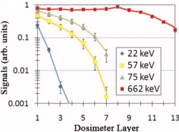
The spectrometer was calibrated at the High Energy X-ray共HEX兲 Laboratory 共NSTec, Livermore, CA兲. The HEX facility produces K-shell line energies by exposing fluores-cent foils to a 160 kV x-ray source. The spectrometer was calibrated with 11 K-shell sources from Zr to Pb, represent-ing line energies of 16 共Zr K␣兲 to 85 共Pb K兲 keV. The photon flux was measured using a Canberra high-purity ger-manium detector previously calibrated with NIST-traceable sources. Additionally, the spectrometer was calibrated with a Cs-137 source共662 keV photon兲 at the Radiation Calorim-etry Laboratory at the Lawrence Livermore National Labo-ratory to provide a single high energy calibration point. The dosimeter signals were compared to one-dimensional Monte Carlo simulations of the filter stack calculated using the Monte Carlo code Integrated Tiger Series 3.0共ITS 3.0兲.23The simulations were used to generate a spectrometer response matrix共SRM兲, representing the dose on each IP for incident photons from 1 keV to 100 MeV energies. Figure2 shows the calibration for four of these data points, at 22, 57, 75, and 662 keV. The data points are the IP readouts and the solid lines represent the predictions of the Monte Carlo model, normalized to the data. The responses are scaled to show them on the same plot. The calibration data show that the Monte Carlo model is a good representation of the response
function. Additionally, the absolute calibration factor deter-mined from scaling the model to the data was found to be consistent for each of the exposures. This calibration factor scales the readout from scanner units to an absolute energy deposition in the IPs.
IV. EXPERIMENTAL DATA
The data from the Bremsstrahlung spectrometer are scanned images of the 13 IPs with a projection of the colli-mator hole on each one. Figure3共a兲shows a sample of six of these channels. For each of the IP channels the mean is taken as the signal level for that channel. The error in the signal level for each channel is quantified as the quadrature addition of three different parameters: the standard deviation in each channel, the gradient across the projection, and a 3% re-sponse variability in the IP scanner. The standard deviation about the mean in each channel is related to the uniformity of the dose and thus the statistics of the deposition. The gradi-ent is taken as the difference in the mean across differgradi-ent parts of the image共away from the boundary兲 and is a mea-sure of three-dimensional 共3D兲 effects in the spectrometer modeling. The 3% IP response variability is empirically de-termined from shot to shot calibration exposures. Figure3共b兲 shows sample data for a 18 J shot and a 121 J shot. The cutoff energy and the slope of the dosimeter signals clearly indicate a trend toward an increasing Bremsstrahlung slope temperature with increasing laser intensity. The signals and errors from each of the spectrometer channels, together with the Monte Carlo modeled SRM, constitute a “few channel spectrometer” problem. The unfolding of the photon spec-trum is described later in this paper.
The K␣data from the single hit spectrometer are shown in Fig. 4. The CCD image was processed using a “single event” algorithm where only photons which deposit all of their energy in a single pixel are counted. The yield is cal-culated by factoring in the detection efficiency of the chip共as a function of chip crowding兲, the solid angle, and filter
trans-FIG. 3. 共Color online兲 Data extraction from the HXBS channels. 共a兲 The mean signal in each channel is taken as the PSL signal value. The error bar on each channel is the quadrature sum of the standard deviation in each channel, the gradient across the channel, and a 3% IP scanner response variation.共b兲 Sample data for a 18 J shot and a 121 J shot. The cutoff energy and the slope of the dosimeter signals clearly indicate a trend toward an increasing Bremsstrahlung slope temperature with increasing laser intensity.
FIG. 4. 共Color online兲 共a兲 The K␣ data from the single hit spectrometer. These yields are not corrected for the opacity of the target and are consid-ered the number of photons escaping from the target at the view angle of the spectrometer. The blue diamonds show the yield in units of photons/SR and the red squares represent the same data normalized to the laser energy. The
K␣yield scales with the laser energy. The normalized yields are plotted on a linear axis to highlight a shot to shot variation up to 30%.
FIG. 2.共Color online兲 The Bremsstrahlung spectrometer is calibrated from 15 to 85 keV and at 662 keV. The points are the measured dosimeter signals and the solid lines represent the Monte Carlo model predictions. The signals are scaled to show them on the same plot. The absolute calibration factor is consistent across the spectrum.
missions. The calculated yields have an error bar of 20% based on the statistics of the signal and on the error in the detection efficiency as calibrated by Maddox et al.22 These yields are not corrected for the opacity of the target and are considered the number of photons escaping from the target at the view angle of the spectrometer. The blue diamonds show the yield in units of photons/SR and the red squares represent the same data normalized to the laser energy. The normalized yields are flat with the laser energy, which shows that the K␣ yield scales linearly with the laser energy. The normalized yields are plotted on a linear axis to highlight the shot to shot variation, which is up to 30%.
V. TARGET SIMULATION
The Bremsstrahlung and K-shell emission from the electron-target interaction was modeled in 3D using an ITS
simulation. 81 narrow spectral bins of electrons logarithmi-cally spaced from 10 keV to 100 MeV are injected at the target surface in a 30 m spot. The electron beam direction-ality and electron cone angle are variable parameters in the simulation. The beam direction is varied between 0° and 16°, consistent with experiments by Santala et al.,24 who found that the beam direction varied between TN to along the laser axis共LA兲 depending on the preformed plasma scale length. The electron cone angle was assumed to have a distribution based on the classical electron ejection angle of electrons in a laser field25 (half= tan−1兵关2/共␥− 1兲兴1/2其). This assumption follows work by Stephens,26where images from buried fluo-rescent foils showed a broad 70– 100 m K␣ spot up to 100 m depth, followed by a 40° 共full兲 divergence angle. From Monte Carlo simulations the assumption of the classi-cal ejection angle was consistent with the measured cone angle distribution. For reference a constant 40° full cone angle response was also simulated. Recent hybrid-PIC simu-lations by Honrubia and Meyer-ten-Vehn27 found that initial electron cone angles consistent with the classical ejection angle reproduced mean divergence angles of 30°–40° seen in experiments due to magnetic collimation effects. The net propagation angle in Monte Carlo simulations is not reduced by collimation so the initial cone angle is expected to be bounded by these two parameter choices.
For each combination of simulation parameters and spectrometer locations, a target response matrix 共TRM兲 is generated, representing the Bremsstrahlung emission from the target for the injected electron energies. The Bremsstrah-lung spectrum is averaged over 5° polar angular bins and 20° azimuthal bins for the off-axis directionality. The K␣ emis-sion detected by the single hit spectrometer is also calcu-lated, generating a K␣ response matrix 共K␣RM兲 for each parameter combination.
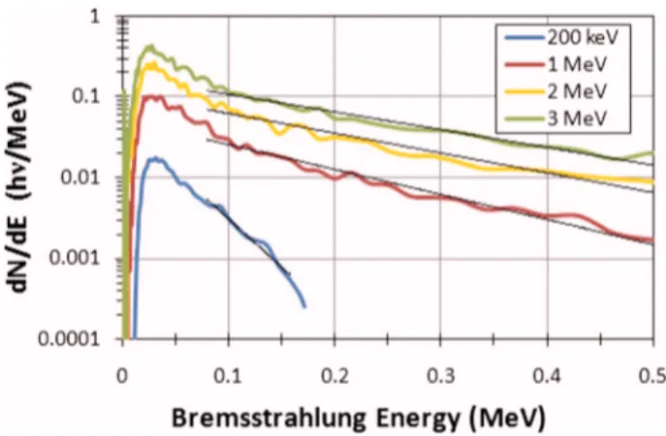
From this model, the Bremsstrahlung emission for vari-ous electron energies is plotted in Fig.5 up to the 500 keV differential photon sensitivity of the spectrometer. There is a clear distinction between 200 keV, 1 MeV, and 2 MeV. Be-tween 2 and 3 MeV the photon spectrum starts to look simi-lar in the energy range of the spectrometer. The 500 keV differential photon sensitivity of the spectrometer thus maps a 2–3 MeV differential electron sensitivity.
The SRM and TRM are multiplied together for the over-all response matrix, representing the response of the dosim-eter layers to electrons injected into the target. This consti-tutes a classic few channel spectrometer problem and the electron spectra can be unfolded using a number of tech-niques, such as fitting test distributions, maximum entropy methods, or singular value decomposition. Here, one and two temperature test distributions seen in previous experimental and computational work13,15,28 are used to determine the band of spectra consistent with the data.
VI. ELECTRON SPECTRUM UNFOLDING AND COMPARISONS TO SCALING LAWS A. One temperature parametrizations
Previous comparisons to intensity scaling laws10,12,13 typically compared a single electron slope temperature共Thot兲 to a single intensity parameter used to characterize the laser. If this is done with the data here, a single electron slope temperature provides a good fit to the Bremsstrahlung data. The fit is characterized by the weighted, reduced 2 fitting parameter, where2⬍1 means on average the predictions fit the measured data within their error bars. The single slope temperature distributions fit the data within 12. The beam directionality is set by the requirement that the electron slope temperature must be simultaneously consistent for both spec-trometers. If the assumed directionality is along the TN, the spectrometer along TN will infer a lower temperature than the spectrometer along the LA. For a given measured spec-trum, the LA spectrometer assumes the actual spectrum is harder since it is not measuring the center of the beam. If the beam directionality is taken along the LA, the TN spectrom-eter likewise assumes a harder spectrum. The beam direction is taken as the angle at which the predicted temperatures are equal. The best fit temperature is thus taken as the tempera-ture that is simultaneously consistent with the measurements from both spectrometers. This works better for higher inten-sities since the electron cone angle is more directional. For
FIG. 5. 共Color online兲 The Bremsstrahlung emission for various electron energies up to the 500 keV differential sensitivity of the spectrometer. There is a distinction between 200 keV, 1 MeV, and 2 MeV. Between 2 and 3 MeV the photon spectrum converges in the energy range of the spectrometer. The 500 keV differential photon sensitivity of the spectrometer maps a 2–3 MeV differential electron sensitivity.
low intensities and consequently lower energy electrons, the assumed cone angle is almost 2and the beam directionality does not matter. The calculated beam directionality varied from 6° to 16°.
Using the FWHM-averaged peak intensity as previously discussed, the slope temperatures are consistent with Beg scaling关Thot= 215共I182兲1/3 keV兴 up to 2⫻1019 W/cm2and 20%–40% higher than Beg scaling for intensities up to 8 ⫻1019 W/cm2. For the 121 J shot shown in Fig. 3共b兲, the single-temperature fit has a Thotof 1.3⫾0.1 MeV. Beg scal-ing predicts a 0.9⫾0.1 MeV Thot 共error bar from the pulse length uncertainty兲, about 40% lower 共2= 10兲. Ponderomo-tive scaling predicts 3.3 MeV, significantly hotter 共2⬇70兲 than the single temperature fit.
This seems to suggest that Beg scaling provides a better fit to the data than ponderomotive scaling. However, this analysis is misleading for two reasons. First, the electron distributions that fit the data are not unique. Parametrization with two temperature components show that different spectra consistent with the data can be drastically different, as will be discussed shortly. Second, comparisons to scaling laws using a single intensity parameter are simplistic and do not properly account for the intensity distribution. The pondero-motive potential is a local effect and proper estimates of the electron spectrum must account for the focal spot intensity distribution rather than just a single peak intensity. Empirical scalings like the Beg scaling law correlate the slope tempera-ture with a defined intensity, as long as a consistent intensity definition is used共which is not always the case兲. This should more consistently predict the slope temperature. However, it is not clear that the intensity scaling law should necessarily translate to other laser systems where the focal spot profile may be very different. Scaling law comparisons using the focal spot intensity distribution will be discussed later in this section.
B. Two temperature parametrizations
The spectral space of the electron distributions can be expanded by parametrizing the distribution using hot and cold temperatures and a ratio between the two components, taking the form f共E兲⬀R共E兩Tc兲+共E兩Th兲, where Tcand Th
are varied from 10 keV to 10 MeV, R from 0.1 to 1000, and
is a normalized Boltzmann or one-dimensional relativistic Maxwellian distribution. The target response matrix with a beam directionality selected from the one-temperature fits is used. The matrix response model simplifies testing of the entire parameter space. The fitting parameter is calculated for 16⫻106 distributions per shot, providing highly resolved variances of the distribution. The electron distributions that simultaneously fit both the spectrometers within 1 2 are selected as valid fits.
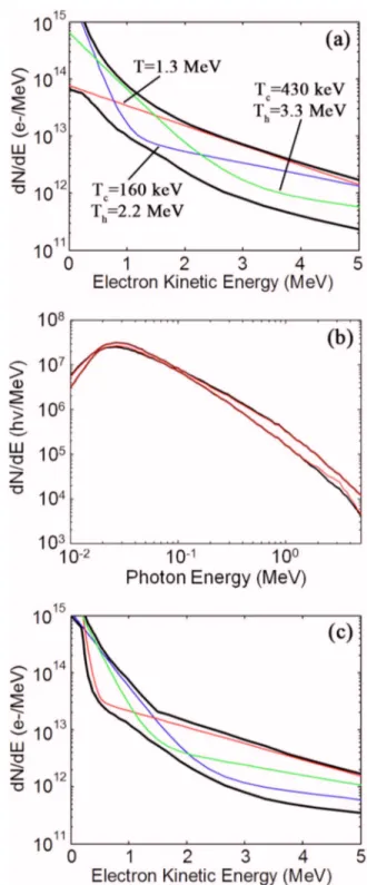
Figure 6共a兲 shows a sample subset of allowed distribu-tions for a 121 J shot, represented by the color lines, along with the envelope of fits, represented by the solid black lines. A broad range of electron distributions is consistent with the data, with almost an order of magnitude difference in the number of electrons at any given energy. The straight red line in Fig.6共a兲represents a single temperature distribution with
a 1.3 MeV slope temperature. The other sample distributions show, however, that this single temperature is not unique and depends on the energy range in which the slope is measured. The solid black lines define the envelope in which the
two-FIG. 6.共Color online兲 共a兲 Various 2-T electron spectra are consistent with the spectrometer data. A sample subset of these curves is plotted, with the black lines representing the envelope of these curves.共b兲 The black lines represent the resultant Bremsstrahlung spectra from the electron spectra in 共a兲. The Bremsstrahlung is significantly more constrained, with the different electron spectra in共a兲 producing the same Bremsstrahlung emission. The red lines represent the Bremsstrahlung spectra from the K␣constrained electron energy spectra.共c兲 2-T electron spectra consistent with both the Bremsstrah-lung data and the K-shell emission. The K-shell emission acts as an electron counter that further constrains the set of possible distributions.
temperature共2-T兲 solutions fall. The envelope itself is not a solution. The envelope serves to bound the spectral space for this shot.
All of these electron distributions generate similar pho-ton spectra up to the differential sensitivity limit of the spec-trometer. The solid black lines in Fig.6共b兲 represent the en-velope of Bremsstrahlung distributions generated by the different electron spectra. This envelope is significantly nar-rower; similar Bremsstrahlung spectra can be generated with larger numbers of colder electrons or smaller numbers of hotter electrons. Above 500 keV the spectrometer has no differential sensitivity, but the Bremsstrahlung spectrum is restricted by the assumption of an exponentially falling elec-tron distribution共in the 2-T parametrization兲.
The band of unfolded electron spectra was reduced by using the Cu K␣emission from the fluorescence layer as an additional constraint. For this shot the measured K␣ yield was 5.3⫻1011⫾20% photons/SR. This yield is not corrected for the target opacity since the opacity is already factored into the K␣RM through the Monte Carlo simulation. The K␣ signal effectively acts as a counter of electrons above 50 keV; these have sufficient energy to reach the copper layer and efficiently stimulate fluorescence. With the K␣ con-straint, the range of possible electron distributions is further reduced in the lower energy part of the spectrum, as shown in Fig.6共c兲. The photon spectrum is only mildly affected, as seen in the solid red lines in Fig.6共b兲.
C. Scaling law comparisons using synthetic electron distributions
A better comparison to analytic scaling laws can be done by generating a synthetic spectrum from the vacuum focal spot intensity distribution. Any modifications due to self-focusing in the preformed plasma are not included here. The intensity distribution is binned in time and space using the focal spot image and a 0.7 ps Gaussian temporal profile as measured from the autocorrelator trace. A conversion effi-ciency and electron energy spectrum are then assigned to each intensity element in space and time using an exponen-tial distribution with a slope temperature from the scaling law and a given conversion efficiency model. Here the flat coupling inferred by Myatt et al. and Nilson et al. is used, with the coupling efficiency scaled to the measured data 共al-ternatively Yasuike’s 10%–50% coupling efficiency would make the hot tail of the electron distribution slightly hotter and would increase the discrepancy shown later between the measured data and the ponderomotive model for tempera-ture兲. The synthetic distribution is then generated by integrat-ing these electron distributions in space and time. This spec-trum does not have a single temperature and the slope temperature is higher when measured at higher energies.
Synthetic electron distributions were generated for three intensity scaling models: ponderomotive scaling, pondero-motive scaling reduced by a 75% scale factor, and the pa-rametrization of density gradient steepening by Chrisman et al.8
The original 1992 PIC simulations of Wilks et al.6 on ponderomotive scaling show a +/−25% difference in
elec-tron temperatures about the ponderomotive potential for p-and s-polarized light, respectively. A synthetic spectrum can then be generated by reducing the ponderomotive tempera-ture by a scale factor, i.e., Th= fTPOND. Since this experiment was performed with a near-normal, s-polarized laser, a syn-thetic spectrum using f = 75% is thus considered within the “error bar” of ponderomotive scaling.
Recent simulations by Chrisman et al.8and Kemp et al.7 have shown a reduction in the slope temperature due to light pressure induced steepening of the density gradient. This arises from shortening of the j⫻B acceleration distance by a factor of
冑
␥nc/nS, where ns is the density of the steepenedshelf. From two-dimensional PIC simulations, the energy spectrum was parametrized by splitting the hot electrons into two components, one with a slope temperature equal to the ponderomotive potential and the other reduced by the factor
冑
␥nc/nS, with each component containing half of theelec-tron energy.
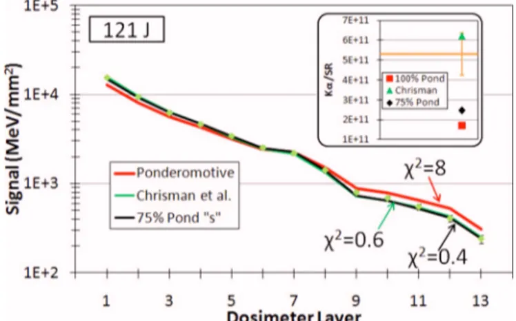
The synthetic spectra generated from these three models are compared to the experimental data in Fig.7. The main figure shows the comparison to the Bremsstrahlung data, while the inset shows the comparison to the measured K␣ signal. The synthetic ponderomotive spectrum is still slightly hotter than the data共2= 8兲, but the fit is significantly better than the 3.3 MeV single temperature ponderomotive distri-bution. The Chrisman parametrization and the 75% pondero-motive model fit the measured data within the error bars. The Bremsstrahlung spectrum predicted by the Chrisman and 75% ponderomotive models are almost exactly the same up to the differential sensitivity limit of the spectrometer. The K␣ signal is shown in the insert by the horizontal orange line, with its associated 20% error bar. The ponderomotive spectrum and the 75% ponderomotive spectrum underpredict the K␣signal by about a factor of 2. The Chrisman param-etrization is consistent with the measured K␣ signal within its error bars.
FIG. 7. 共Color online兲 The synthetic spectra derived from different Thot
scalings using the focal spot intensity distribution are fit to the measured Bremsstrahlung data for the 121 J shot. The synthetic ponderomotive spec-trum is slightly hotter than the data. The Chrisman parametrization and 75% synthetic ponderomotive spectrum fit the Bremsstrahlung data within the error bars. The inset shows the K␣predictions of the different spectra rela-tive to the measured data, given by the orange line and error bars. The ponderomotive and 75% ponderomotive spectra underpredict the K␣signal by a factor of 2.
The Chrisman parametrization provides the best fit to both the Bremsstrahlung and K␣ data in this Monte Carlo model. Resistive transport effects neglected in the Monte Carlo simulations are a potential source of uncertainty and will be assessed later in this paper.
VII. CONVERSION EFFICIENCY SCALINGS WITH INTENSITY
The total conversion efficiency共L→e−兲 and the
conver-sion efficiency into 1–3 MeV共L→1–3 MeVe−兲 electrons is
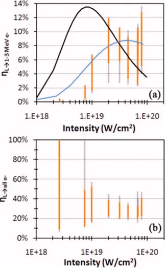
cal-culated for each of the 2-T distributions previously de-scribed. Figure8共a兲shows the scaling ofL→1–3 MeVe−with
laser intensity. The solid gray bars represent the predicted conversion efficiencies for the spectra that fit the Bremsstrah-lung data with 12; the orange bars also fit the K␣constraint within its 20% error bars. L→1–3 MeVe− peaks around 2
⫻1019 W/cm2and then falls off. The conversion efficiency into 1–3 MeV electrons is banded between 3%–12%. For reference, the black and blue lines represent conversion
effi-ciencies into 1–3 MeV electrons given ponderomotive scal-ing applied to a sscal-ingle peak intensity and a representative vacuum focal spot distribution, respectively, and a 25% total conversion efficiency. With standard ponderomotive scaling,
L→1–3 MeVe−peaks at too low an intensity compared to the
data, suggesting that the calculated spectrum needs to take into account both the focal spot distribution and a possible reduction in the temperature. The blue line takes the vacuum focal spot into account, and predicts a flat coupling to 1–3 MeV electrons for laser intensities of 2⫻1019–8⫻1019 W/cm2. The total conversion efficiencies are shown in Fig.8共b兲. The total conversion efficiencies are banded between 20% and 40%. This is slightly higher than the 10%–30% minimum conversion efficiencies measured by Nilson et al., which is probably due to their neglect of energy transfer to fast ions.
The conversion efficiencies predicted from the synthetic spectra from the various scaling models are shown in TableI. For the 121 J shot, the electron distributions consistent with both the Bremsstrahlung spectrum and the K␣ constraint bound L→e− between 20% and 31% and L→1–3 MeVe−
be-tween 2.5% and 7.7%. The synthetic ponderomotive spec-trum results in a total conversion efficiency lower than these bounds共while the distribution shape is given by the models, the absolute conversion efficiency is scaled to the data兲. The Chrisman conversion efficiencies are calculated to be
L→e−= 25% and L→1–3 MeVe−= 4.6%. The higher
conver-sion efficiency is due to the larger number of prescribed colder electrons, which contribute to the energy of the spec-trum but do not produce significant levels of Bremsstrahlung. At these intensities, the Chrisman parametrization has essen-tially the same energy fraction of 1–3 MeV electrons as the ponderomotive scaling. At higher intensities required for ig-nition, more of the low energy component of the spectrum would fall in the energy range of interest so the useful frac-tion would increase.
The 75% ponderomotive spectrum results in more en-ergy going into 1–3 MeV electrons by reducing the tempera-ture of the higher energy tail. This model does not prescribe a large bulk of low energy electrons that inflate the total conversion efficiency of the Chrisman model.
VIII. DISCUSSION AND SYSTEMATIC UNCERTAINTIES
The requirements for ignition have been the subject of several modeling studies.5,27,29Atzeni et al.5assumes for ex-ample a 25% total conversion efficiency and a hot electron temperature consistent with ponderomotive scaling, resulting
FIG. 8.共Color online兲 共a兲 The conversion efficiency into 1–3 MeV electrons is plotted vs laser intensity. The gray bars represent the predicted conversion efficiencies from the Bremsstrahlung data. The orange bars represent the conversion efficiencies also consistent with the K␣ measurement. Above 1019 W/cm2, about 3%–12% of the laser energy goes into 1–3 MeV
elec-trons. For reference, the black and blue lines represent conversion efficien-cies into 1–3 MeV electrons given ponderomotive scaling applied to a single peak intensity and a representative vacuum focal spot distribution, respec-tively, and a 25% total conversion efficiency.共b兲 Laser conversion efficien-cies into all electrons range from 20% to 40% for intensities above 1019 W/cm2.
TABLE I. Conversion efficiencies for the synthetic electron spectra for the 121 J shot. Model L→e− 共%兲 L→1–3 MeVe − 共%兲 2-T parametrization 20–31 2.5–7.7 Ponderomotive 16 5.3 75% ponderomotive 20 6.9 Chrisman 25 4.6
in electrons with too large a range for optimal coupling to the hot spot. The total conversion efficiency measured here is consistent with that assumption, with electron temperatures giving a more optimal range, suggesting somewhat more fa-vorable conditions. The conversion efficiency into 1–3 MeV electrons reported here is low. In this experiment, this is due to the large amounts of energy in the low intensity wings of the focal spot, suggesting the focal spot profile is an impor-tant consideration in a fast ignition driver. The cone angle assumed here, however, ranges from 90° to 60° for 1–3 MeV electrons. This would result in a transport cone angle worse than usually assumed in modeling of ignition. Magnetic fo-cusing of the electron beam at ignition scale conditions miti-gates the effect of divergence of the source electrons and is a subject of ongoing study.30,31
There are two primary sources of error that systemati-cally bias this analysis: the assumption of the electron cone angle and the neglect of resistive transport effects. In contrast with the classical ejection angle assumption, if all the elec-trons are launched into a 40° cone angle whether by mag-netic collimation or otherwise, the calculated conversion ef-ficiencies for the 121 J shot would beL→e−= 16% – 22% and
L→1–3 MeVe−= 1.6% – 5.4% 共with the K␣ constraint兲. The
full conversion efficiency is 25% lower and the conversion efficiency into 1–3 MeV electrons is reduced by 30%–40%. The angular distribution of the electrons is the main uncer-tainty in unfolding the electron spectrum from the Brems-strahlung measurements. A full spectral and angular mea-surement, similar to work by Schwoerer et al.,32or imaging of multiple fluorescent layers buried in the target could help provide additional constraints on the angular distribution.
The other source of error is the neglect of collective electric and magnetic effects in the transport model. While collective fields are not present in a basic Monte Carlo model, the impact can be estimated using a Bell-like33model where an Ohmic potential drives a return current of thermal electrons. The magnitude of the potential in these experi-ments is estimated using an initial electron spectrum from the Chrisman parametrization applied to the focal spot inten-sity distribution and a 25% conversion efficiency, as de-scribed above. The electrons are binned into energy groups and are launched from a 30 m diameter spot into a cone angle given by the classical ejection angle. The electric field is given by E共z兲 =共z兲j共z兲 =共z兲
兺
i Nie 1 共r0+ z tani兲2 H共Ri− z兲,whereis the resistivity of the material, Niis the number of
electrons in each energy group, r0is the initial spot size,iis the divergence angle of each energy group, H is the Heavi-side step function, and Riis the range of the electrons in each
energy group.
The electric field is calculated as a function of depth with a cutoff at the electron range. The electrons lose energy through collisional, radiative, and resistive effects. The col-lisional and radiative losses are taken from tabulated values for cold matter.34 Scattering is included in a rough way by taking the electron path length as two times greater than the
linear penetration depth 共in Al兲, which has been shown for energies from 10 keV to several MeV.35,36The electron range is thus approximated by integrating the energy loss against the potential into the target along with twice the collisional and radiative losses. The electric field is calculated and summed for all energy groups and integrated for a potential across the target. This procedure is then iterated to converge upon a self-consistent solution of the potential and electron penetration depth.
Using this formulation, the potential across the target is calculated at 700 kV if a peak aluminum resistivity of about 1.5⫻10−6 ⍀ m is used for the entire bulk, assuming that most of the interactions occur at temperatures between 10 and 100 eV for which the resistivity of Al is close to the peak value. Half of the potential is in the first 10 m and 34 is in the first 30 m, before the electrons have had a chance to spread. The calculated potential is temperature dependent and may be lower depending on the actual temperature dis-tribution in the target. 3D currents may also serve to partially lower the front surface charge buildup and thus reduce the potential felt by the hot electrons. Regardless, given the elec-tron currents in these experiments, the potential is likely to be at least a couple hundred kV.
Neglecting this potential in a Monte Carlo analysis may influence the interpretation of the conversion efficiencies. Since the majority of the potential is in the first few tens of microns and the Bremsstrahlung is produced throughout the bulk, all of the electrons producing Bremsstrahlung in the target pass through this potential. The electron spectrum is essentially downshifted by this potential before it produces Bremsstrahlung. The electron spectrum inferred from the measured Bremsstrahlung emission just needs to be up-shifted by the potential. If the mean energy is taken as the 1.3 MeV single temperature fit, a shift of a couple hundred kV would slightly perturb the inferred conversion efficiencies. The synthetic ponderomotive spectrum discussed in Sec. VI C is also within range of this potential Ohmic correction. Transport simulations similar to those by Davies18and Hon-rubia and Meyer-ten-Vehn27 are necessary to quantify the shift in the spectrum. The K␣emission is strongly influenced by the Ohmic potentials, as previously discussed by Davies. With the Monte Carlo analysis, the fluor acts as a counter of electrons above 50 keV. If there is a potential of a few hun-dred kV in the first ten microns before the fluor, the energy at which this counter acts is upshifted to a few hundred keV. This could slightly downshift the number of K␣photons pre-dicted by the different models.
The impact of the Ohmic potentials on the K␣constraint is mixed. Some of the electron spectra in Fig. 6共a兲 with larger numbers of electrons in the hundred of keV range produce too much K␣in the Monte Carlo model to be con-sistent with measured K␣ emission. With an Ohmic model, these distributions would be consistent with the data. This would result in an upward revision of the total conversion efficiency since there would be larger numbers of low energy electrons. The conversion efficiency into 1–3 MeV electrons is likely to drop since fewer high energy electrons would be needed to produce the measured Bremsstrahlung emission. Graphically, the orange bars in Fig.8共b兲will shift upwards,
slightly increasingL→e−, while still subject to the
Brems-strahlung constraint indicated by the gray bars. The orange bars in Fig. 8共a兲 will shift downwards, reducing
L→1–3 MeVe−.
Magnetic fields may enhance the energy loss near the front surface of the target and reduce the penetration lengths by increasing the curvature of the electron path.18The impact of magnetic fields on the conversion efficiency would thus be analogous to that of the Ohmic potential.
IX. CONCLUSIONS
The Bremsstrahlung spectrum and K␣ emission of a fluorescent layer have been measured in nonrefluxing targets. Through Monte Carlo modeling, conversion efficiencies into 1–3 MeV electrons of 3%–12% have been inferred. This rep-resents a total conversion efficiency of 20%–40%. Assump-tions of the angular distribution model are a major source of uncertainty in the analysis. Better comparisons to scaling laws used synthetic energy spectra generated from the inten-sity distribution of the focal spot. Forward calculations of the electron spectra for various intensity scaling models were compared to the Bremsstrahlung data. The forward calcula-tions are suggestive of energy spectra with lower slope tem-peratures than scaling with the ponderomotive potential of the laser. Resistive effects result in potentials of a few hun-dred kilovolts in the first tens of microns in the target. This may result in higher total conversion efficiencies than in-ferred from Monte Carlo modeling but lower conversion ef-ficiencies into the 1–3 MeV band of primary interest to fast ignition.
ACKNOWLEDGMENTS
The authors would like to acknowledge Zaheer Ali and Michael Haugh of the HEX facility 共NSTec兲, Bill Carl and Frank Balgos of the RCL, as well as the staff of the Jupiter Laser Facility for their assistance and support during the cali-brations and experiments.
This work was performed under the auspices of the U.S. Department of Energy by Lawrence Livermore National Laboratory under Contract No. DE-AC52-07NA27344 共Au-thorization Review No. LLNL-JRNL-415191兲.
1M. Tabak, J. E. Hammer, M. E. Glinsky, W. L. Kruer, S. C. Wilks, J.
Woodworth, E. M. Campbell, M. Perry, and R. J. Mason,Phys. Plasmas 1, 1626共1994兲.
2M. Tabak, J. H. Hammer, E. M. Campbell, W. L. Kruer, J. Goodworth, S.
C. Wilks, and M. Perry, Lawrence Livermore National Laboratory Patent Disclosure No. IL8826B, 1994; S. Hatchett and M. Tabak, “Cone focus geometry for fast ignition,” in 30th Annual Anomalous Absorption Con-ference, Ocean City, MD, April 2000; S. Hatchett, M. Herrmann, M. Tabak, R. Turner, and R. Stephens, Bull. Am. Phys. Soc. 46, BP1.086 共2001兲.
3R. Kodama, P. A. Norreys, K. Mima, A. E. Dangor, R. G. Evans, H.
Fujita, Y. Kitagawa, K. Krushelnick, T. Miyakoshi, N. Miyanaga, T. Nori-matsu, S. J. Rose, T. Shozaki, K. Shigemori, A. Sunahara, M. Tampo, K. A. Tanaka, Y. Toyama, T. Yamanaka, and M. Zepf,Nature共London兲 412,
798共2001兲.
4R. Kodama, H. Shiraga, K. Shigemori, Y. Toyama, S. Fujioka, H. Azechi,
H. Fujita, H. Habara, T. Hall, Y. Izawa, T. Jitsuno, Y. Kitagawa, K. M. Krushelnick, K. L. Lancaster, K. Mima, K. Nagai, M. Nakai, H. Nish-imura, T. Norimatsu, P. A. Norreys, S. Sakabe, K. A. Tanaka, A. Youssef, M. Zepf, and T. Yamanaka,Nature共London兲 418, 933共2002兲.
5S. Atzeni, A. Schiavi, and C. Bellei,Phys. Plasmas14, 052702共2007兲. 6S. C. Wilks, W. L. Kruer, M. Tabak, and A. B. Langdon,Phys. Rev. Lett.
69, 1383共1992兲.
7A. J. Kemp, Y. Sentoku, and M. Tabak,Phys. Rev. Lett. 101, 075004
共2008兲.
8B. Chrisman, Y. Sentoku, and A. J. Kemp,Phys. Plasmas 15, 056309
共2008兲.
9M. G. Haines, M. S. Wei, F. N. Beg, and R. B. Stephens,Phys. Rev. Lett.
102, 045008共2009兲.
10G. Malka and J. L. Miquel,Phys. Rev. Lett. 77, 75共1996兲.
11K. A. Tanaka, R. Kodama, H. Fujita, M. Heya, N. Izumi, Y. Kato, Y.
Kitagawa, K. Mima, N. Miyanaga, T. Norimatsu, A. Pukhov, A. Sunahara, K. Takahashi, M. Allen, H. Habara, T. Iwatani, T. Matusita, T. Miyakosi, M. Mori, H. Setoguchi, T. Sonomoto, M. Tanpo, S. Tohyama, H. Azuma, T. Kawasaki, T. Komeno, O. Maekawa, S. Matsuo, T. Shozaki, K. Suzuki, H. Yoshida, T. Yamanaka, Y. Sentoku, F. Weber, T. W. Barbee, Jr., and L. DaSilva,Phys. Plasmas 7, 2014共2000兲.
12M. A. Stoyer, T. C. Sangster, E. A. Henry, M. D. Cable, T. E. Cowan, S.
P. Hatchett, M. H. Key, M. J. Moran, D. M. Pennington, M. D. Perry, T. W. Phillips, M. S. Singh, R. A. Snavely, M. Tabak, and S. C. Wilks,Rev. Sci. Instrum. 72, 767共2001兲.
13P. A. Norreys, M. Santala, E. Clark, M. Zepf, I. Watts, F. N. Beg, K.
Krushelnick, M. Tatarakis, A. E. Dangor, X. Fang, P. Graham, T. McCanny, R. P. Singhal, K. W. D. Ledingham, A. Creswell, D. C. W. Sanderson, J. Magill, A. Machacek, J. S. Wark, R. Allott, B. Kennedy, and D. Neely,Phys. Plasmas 6, 2150共1999兲.
14K. Yasuike, M. H. Key, S. P. Hatchett, R. A. Snavely, and K. B. Wharton,
Rev. Sci. Instrum. 72, 1236共2001兲.
15F. N. Beg, A. R. Bell, A. E. Dangor, C. N. Danson, A. P. Fews, M. E.
Glinsky, B. A. Hammel, P. Lee, P. A. Norreys, and M. Tatarakis,Phys. Plasmas 4, 447共1997兲.
16J. Myatt, W. Theobald, J. A. Delettrez, C. Stoeckl, M. Storm, T. C.
Sang-ster, A. V. Maximov, and R. W. Short,Phys. Plasmas 14, 056301共2007兲.
17P. M. Nilson, W. Theobald, J. Myatt, C. Stoeckl, M. Storm, O. V. Gotchev,
J. D. Zuegel, R. Betti, D. D. Meyerhofer, and T. C. Sangster,Phys. Plas-mas 15, 056308共2008兲.
18J. R. Davies,Phys. Rev. E 65, 026407共2002兲.
19B. C. Stuart, J. D. Bonlie, J. A. Britten, J. A. Caird, R. Cross, C. A.
Ebbers, M. J. Eckart, A. C. Erlandson, W. A. Molander, A. Ng, P. K. Patel, and D. F. Price, Tech. Dig. Ser.-Opt. Soc. Am., paper JTuG3共2006兲.
20S. Le Pape, Y. Y. Tsui, A. G. Macphee, D. S. Hey, P. K. Patel, A. J.
Mackinnon, M. H. Key, M. Wei, T. Y. Ma, F. N. Beg, R. B. Stephens, K. U. Akli, A. Link, L. D. Van-Woerkom, and R. R. Freeman, “Characteriza-tion of the preformed plasma for high intensity laser-plasma interac“Characteriza-tion,” Opt. Lett.共to be published兲.
21C. D. Chen, J. A. King, M. H. Key, K. U. Akli, F. N. Beg, H. Chen, R. R.
Freeman, A. Link, A. J. Mackinnon, A. G. MacPhee, P. K. Patel, M. Porkolab, R. B. Stephens, and L. D. Van Woerkom,Rev. Sci. Instrum.79,
10E305共2008兲.
22B. R. Maddox, H. S. Park, B. A. Remington, and M. McKernan,Rev. Sci.
Instrum. 79, 10E924共2008兲.
23J. A. Halbleib, R. P. Kensek, G. D. Valdez, S. M. Seltzer, and M. J. Berger,
IEEE Trans. Nucl. Sci. 39, 1025共1992兲.
24M. I. K. Santala, M. Zepf, I. Watts, F. N. Beg, E. Clark, M. Tatarakis, K.
Krushelnick, A. E. Dangor, T. McCanny, I. Spencer, R. P. Singhal, K. W. D. Ledingham, S. C. Wilks, A. C. Machacek, J. S. Wark, R. Allott, R. J. Clarke, and P. A. Norreys,Phys. Rev. Lett. 84, 1459共2000兲.
25C. I. Moore, J. P. Knauer, and D. D. Meyerhofer,Phys. Rev. Lett. 74,
2439共1995兲.
26R. B. Stephens, R. A. Snavely, Y. Aglitskiy, F. Amiranoff, C. Andersen,
D. Batani, S. D. Baton, T. Cowan, R. R. Freeman, T. Hall, S. P. Hatchett, J. M. Hill, M. H. Key, J. A. King, J. A. Koch, M. Koenig, A. J. MacKin-non, K. L. Lancaster, E. Martinolli, P. Norreys, E. Perelli-Cippo, M. Rabec Le Gloahec, C. Rousseaux, J. J. Santos, and F. Scianitti,Phys. Rev. E 69,
066414共2004兲.
27J. J. Honrubia and J. Meyer-ter-Vehn,Plasma Phys. Controlled Fusion51,
014008共2009兲.
28M. H. Key, M. D. Cable, T. E. Cowan, K. G. Estabrook, B. A. Hammel, S.
P. Hatchett, E. A. Henry, D. E. Hinkel, J. D. Kilkenny, J. A. Koch, W. L. Kruer, A. B. Langdon, B. F. Lasinski, R. W. Lee, B. J. MacGowan, A. MacKinnon, J. D. Moody, M. J. Moran, A. A. Offenberger, D. M. Pen-nington, M. D. Perry, T. J. Phillips, T. C. Sangster, M. S. Singh, M. A. Stoyer, M. Tabak, G. L. Tietbohl, M. Tsukamoto, K. Wharton, and S. C. Wilks,Phys. Plasmas 5, 1966共1998兲.
29R. Betti, A. A. Solodov, J. A. Delettrez, and C. Zhou,Phys. Plasmas 13,
100703共2006兲.
30A. P. L. Robinson and M. Sherlock,Phys. Plasmas 14, 083105共2007兲. 31S. Kar, A. P. L. Robinson, D. C. Carroll, O. Lundh, K. Markey, P.
McKenna, P. Norreys, and M. Zepf,Phys. Rev. Lett. 102, 055001共2009兲.
32H. Schwoerer, P. Gibbon, S. Dusterer, R. Behrens, C. Ziener, C. Reich,
and R. Sauerbrey,Phys. Rev. Lett. 86, 2317共2001兲.
33A. R. Bell, J. R. Davies, S. Guerin, and H. Ruhl,Plasma Phys. Controlled
Fusion 39, 653共1997兲.
34International Commission on Radiation Units and Measurements,
“Stop-ping powers for electrons and positrons,” ICRU Technical Report No. 37, 1984.
35B. F. J. Schonland,Proc. R. Soc. London, Ser. A 108, 187共1925兲. 36R. W. Varder, Philos. Mag. 29, 725共1915兲.