to Travel Demand Analysis
by
John L. Bowman
Submitted to the Department of Civil and Environmental Engineering in Partial Fulfillment of the Requirements for the Degree of
Doctor of Philosophy
in
Transportation Systems and Decision Sciences
at the
Massachusetts Institute of Technology
May 1998© 1998 Massachusetts Institute of Technology All rights reserved
Signature of Author___________________________________________________________ Department of Civil and Environmental Engineering May 22, 1998
Certified by_________________________________________________________________ Moshe Ben-Akiva Edmund K. Turner Professor of Civil and Environmental Engineering Thesis Supervisor
Accepted by________________________________________________________________ Joseph M. Sussman Chairman, Departmental Committee on Graduate Studies
to Travel Demand Analysis
byJohn L. Bowman
Submitted to the Department of Civil and Environmental Engineering on May 22, 1998 in partial fulfillment of the requirements for the Degree of
Doctor of Philosophy in Transportation Systems and Decision Sciences
Abstract
This study develops a model of a person’s day activity schedule that can be used to forecast urban travel demand. It is motivated by the notion that travel outcomes are part of an activity scheduling decision, and uses discrete choice models to address the basic modeling
problem—capturing decision interactions among the many choice dimensions of the immense activity schedule choice set.
An integrated system of choice models represents a person’s day activity schedule as an activity pattern and a set of tours. A pattern model identifies purposes, priorities and
structure of the day’s activities and travel. Conditional tour models describe timing, location and access mode of on-tour activities. The system captures trade-offs people consider, when faced with space and time constraints, among patterns that can include at-home and on-tour activities, multiple tours and trip chaining. It captures sensitivity of pattern choice to activity and travel conditions through a measure of expected tour utility arising from the tour models. When travel and activity conditions change, the relative attractiveness of patterns changes because expected tour utility changes differently for different patterns.
An empirical implementation of the model system for Portland, Oregon, establishes the feasibility of specifying, estimating and using it for forecasting. Estimation results match a priori expectations of lifestyle effects on activity selection, including those of (a) household structure and role, such as for females with children, (b) capabilities, such as income, and (c) activity commitments, such as usual work levels. They also confirm the significance of activity and travel accessibility in pattern choice. Application of the model with road pricing and other policies demonstrates its lifestyle effects and how it captures pattern shifting—with accompanying travel changes—that goes undetected by more narrowly focused trip-based and tour-based systems.
Although the model has not yet been validated in before-and-after prediction studies, this study gives strong evidence of its behavioral soundness, current practicality, potential to generate cost-effective predictions superior to those of the best existing systems, and potential for enhanced implementations as computing technology advances.
Thesis Supervisor: Dr. Moshe Ben-Akiva
Biographical Note
John L. Bowman’s research interests lie in the development of disaggregate models of individual and household lifestyle, mobility, activity and travel behavior, to inform public land use, transport, environmental and welfare policy. He has taught a graduate demand modeling course at MIT.
Dr. Bowman received the degree of Master of Science in Transportation from MIT in 1995, and the degree of Bachelor of Science in mathematics, summa cum laude, in 1977 from Marietta College, Marietta, Ohio. He is a member of Phi Beta Kappa. Before his study of transportation he worked for 14 years in systems development, product development and management for an insurance and financial services firm.
Publications of which Dr. Bowman is co-author include “Travel Demand Model System for the Information Era”, Transportation 23: 241-266, 1996; “Integration of an Activity-based Model System and a Residential Location Model”, Urban Studies 35 (7): 1231-1253, 1998; and “Activity based Travel Demand Models”, in Proceedings of the Equilibrium and
Advanced Transportation Modeling Colloquium, University of Montreal Center for Research on Transport, 1998.
Acknowledgments
This research was supported by the United States Department of Transportation through an Eisenhower Fellowship, with additional funds supplied by federal research grants provided through the New England Region University Transportation Program.
I wish to express gratitude to the many people who contributed directly and indirectly to the completion of this thesis.
Professor Moshe Ben-Akiva, my advisor and committee chairman, first suggested the idea of modeling an entire day’s activity and travel schedule, then provided the guidance I needed to bring it to fruition.
Members of my doctoral committee were very helpful. Professor Michel Bierlaire has supplied many ideas for the direction and content of my research. Professor Rabi Mishalani began giving me welcome guidance and encouragement the first year I arrived at MIT, and has not stopped since. Professor Nigel Wilson gave very helpful comments on my thesis draft.
Mark Bradley has been my partner in research and development. He took my designs and turned them into a practical production system in Portland, provided data I needed for model development, produced forecasts included in this thesis, and wrote early drafts of materials in the thesis related to the Portland model system. Keith Lawton of Portland Metro saw an early version of the day activity schedule model and became the principal sponsor who made
the Portland implementation a possibility. Tom Rossi supported the effort to fund
development of the Portland day activity schedule model through a Cambridge Systematics federal task order contract. I learned much from these three about what it takes to turn academic research into useful innovation.
Staffan Algers, Alex Anas, Kay Axhausen, Chandra Bhat, Ennio Cascetta, Dick Ettema, Konstadinos Goulias, Ryuichi Kitamura, Frank Koppelman, Eric Miller, Taka Morikawa, Kai Nagel, Eric Pas, Yoram Shiftan, Harry Timmermans and Peter Vovsha are academics from around the world who have directly contributed, in one way or another, to the intellectual substance of my work.
Andrew Daly expeditiously increased the capacity of his estimation software, ALOGIT, when I really needed it.
Julie Bernardi has taken care of countless details for proposals, equipment, supplies, papers, reports and presentations leading to this thesis.
Steve Perone, Kyung-Hwa Kim, Karen Larson, Bob Knight and Phil Wuest of Portland Metro provided me with data I needed and some of them accepted the task of taking my work immediately from the research laboratory into a real world application.
Professor Ismail Chabini gave enthusiastic support of me and my work, and insightful suggestions on presenting them to others.
Professor Joseph Sussman provided encouragement throughout my stay at MIT.
Kevin Tierney, Kimon Proussaloglou, Earl Ruiter and Nagaswar Jonnalagada, colleagues at Cambridge Systematics, made my summers enriching, enjoyable and important times of intellectual ferment.
John Abraham, Reinhard Clever, Sean Doherty, Shinwon Kim, Catherine Lawson, Jun Ma, Amr Mahmoud and Jack Wen are fellow students in my field with whom I’ve enjoyed discussing ideas.
Kazi Ahmed, Kalidas Ashok, Omar Baba, Adriana Bernardino, Jon Bottom, Chris Caplice, Jiang Chang, Owen Chen, Yan Dong, Prodyut Dutt, Xu Jun Eberlein, Andras Farkas, Dinesh Gopinath, Mark Hickman, Hong Jin, Daeki Kim, Amalia Polydoropoulou, Scott Ramming, Daniel Roth, Dan Turk, Joan Walker and Qi Yang are current and former fellow
transportation students at MIT, with whom I have shared stimulating conversation and the camaraderie of graduate student life.
Finally, I thank my wife, Joanne, for her unfailing support, my children, Sarah and Phillip, for their patience throughout the last six years, and my parents, Roy and Verna, for teaching me to pursue my dreams.
Contents
ABSTRACT... 3 BIOGRAPHICAL NOTE... 5 ACKNOWLEDGMENTS... 5 CONTENTS... 7 FIGURES... 10 TABLES... 111 INTRODUCTION AND SUMMARY ... 13
1.1 INTRODUCTION... 13
1.2 SUMMARY... 16
1.2.1 Theory of activity-based travel demand ... 16
1.2.2 Models of activity and travel scheduling... 17
1.2.3 Discrete choice modeling approaches ... 19
1.2.4 The day activity schedule model system... 20
1.2.5 The Portland day activity schedule model system ... 22
1.2.6 Model application and evaluation ... 25
1.2.7 Conclusions... 27
1.2.8 Research topics ... 28
1.2.9 Outline of the thesis ... 29
2 THEORY OF ACTIVITY-BASED TRAVEL DEMAND... 31
2.1 THE CHARACTERISTICS OF ACTIVITY AND TRAVEL DEMAND... 31
2.2 ACTIVITY AND TRAVEL DECISION FRAMEWORK... 34
2.3 LIFESTYLE BASIS OF ACTIVITY DECISIONS... 38
2.4 THE CHOICE PROCESS AND THE COMPLEXITY OF THE ACTIVITY SCHEDULING DECISION... 40
2.5 BEHAVIOR-THEORETICAL MODELING REQUIREMENTS... 43
3 MODELS OF ACTIVITY AND TRAVEL SCHEDULES ... 45
3.1 MODEL SYSTEM REQUIREMENTS... 45
3.2 OVERVIEW OF MODELING APPROACHES... 46
3.3 RULE-BASED SIMULATIONS... 49
3.3.1 STARCHILD: classification and choice... 49
3.3.2 AMOS: search for a satisfactory adjustment... 51
3.3.3 SMASH: sequential schedule building ... 55
3.3.4 Summary evaluation of rule-based simulations... 56
3.4 DISCRETE CHOICE MODELS... 57
3.4.1 Discrete choice methods ... 57
3.4.2 Trips and tours ... 58
3.4.3 Trip-based system... 59
3.4.4 Tour-based system ... 61
3.4.5 Summary evaluation of trip and tour-based discrete choice model systems ... 64
4 THE DAY ACTIVITY SCHEDULE MODEL SYSTEM ... 65
4.1 INTRODUCTION AND OVERVIEW OF THE MODEL SYSTEM... 65
4.2 MATHEMATICAL FORM OF THE MODEL SYSTEM... 69
4.2.1 Day activity schedule probability ... 69
4.2.2 Pattern model ... 70
4.2.3 Tour model ... 71
4.2.4 Tour model details... 71
4.3 MODEL DESIGN ISSUES... 72
4.3.1 Conditional independence... 72
4.3.2 Additive expected maximum utility ... 73
4.3.4 Choice set generation ... 74
4.3.5 Lifestyle outcomes versus day activity schedule choices... 75
5 THE PORTLAND DAY ACTIVITY SCHEDULE MODEL SYSTEM... 77
5.1 INTRODUCTION... 77
5.2 DEVELOPMENT HISTORY... 78
5.3 THE PORTLAND SAMPLE DATA... 79
5.4 DAY ACTIVITY SCHEDULE MODEL SYSTEM... 82
5.5 TOUR MODELS... 84
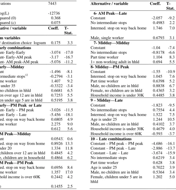
5.5.1 Home-based tour time-of-day models... 85
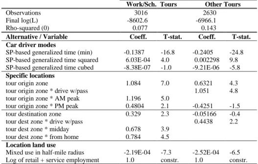
5.5.2 Home-based tour primary destination and mode choice models... 89
5.5.3 Work-based subtour and intermediate stop models... 93
5.6 DAY ACTIVITY PATTERN MODEL... 96
5.6.1 Pattern model choice set... 96
5.6.2 Pattern model utility functions—components and variables ...102
5.6.3 Summary of pattern model estimation results ...106
5.6.4 Primary activity components...108
5.6.5 Secondary activity components ...112
5.6.6 Pattern components ...116
5.6.7 Tours accessibility...124
5.6.8 Pattern model specification tests...125
5.7 EMPIRICAL ISSUES...128
5.7.1 Conditional independence ...128
5.7.2 Resolution of choice dimensions ...128
5.7.3 Integration across the conditional hierarchy ...130
5.7.4 Survey data ...130
6 MODEL APPLICATION AND EVALUATION ...137
6.1 MODEL SYSTEM APPLICATION PROCEDURES...137
6.1.1 Basic procedures and variations ...137
6.1.2 Portland production system application procedures ...139
6.1.3 Simplified procedure for model demonstration ...141
6.2 PEAK PERIOD TOLL POLICY...141
6.2.1 Policy and expected behavioral response ...141
6.2.2 Activity pattern effects ...142
6.2.3 Travel effects...144
6.2.4 Heterogeneity of activity patterns and pattern effects ...147
6.3 IMPROVED TRANSIT ACCESS...150
6.3.1 Transit access improvement without restricted auto ownership...151
6.3.2 Transit access improvement with auto ownership restriction ...153
6.4 OTHER POLICY APPLICATIONS...154
6.4.1 Demand management ...154
6.4.2 Spatial accessibility improvements...155
6.4.3 Highway service level changes ...157
6.4.4 Telecommunications ...157
6.5 CONCLUSIONS...158
7 CONCLUSIONS AND RECOMMENDATIONS ...161
7.1 CONCLUSIONS...161
7.1.1 Theoretical model...161
7.1.2 Empirical model ...163
7.1.3 Model application results ...164
7.2 RECOMMENDATIONS...166
7.2.1 Model validation ...167
7.2.2 Application procedures...167
7.2.4 Model enhancement using merged data from evolving surveys... 169
7.2.5 Survey design and data collection methods... 169
7.2.6 Computational efficiency, application methods and alternative decision protocols... 170
7.2.7 Integrated activity and mobility models ... 170
7.2.8 Theoretical research... 171
APPENDIX A TRANSLATION OF SURVEY DATA INTO DAY ACTIVITY PATTERNS... 173
APPENDIX B THE PORTLAND 114 ALTERNATIVE DAY ACTIVITY PATTERN MODEL... 179
BIBLIOGRAPHY... 181
Figures
Figure 1.1 Activity schedule adjustments to a peak period toll...15
Figure 1.2 The day activity schedule ...21
Figure 1.3 Portland day activity schedule model system ...23
Figure 2.1 Activity and travel decision framework ...34
Figure 3.1 STARCHILD model system ...50
Figure 3.2 AMOS model system ...52
Figure 3.3 A portion of the AMOS context specific search ...54
Figure 3.4 SMASH model system ...55
Figure 3.5 Trip and tour-based model subdivision of the day activity schedule ...59
Figure 3.6 The MTC trip-based model system ...60
Figure 3.7 The Stockholm tour-based model system ...62
Figure 3.8 The Stockholm nested logit work tour model ...62
Figure 3.9 The Stockholm shopping tours model ...63
Figure 4.1 The day activity schedule ...67
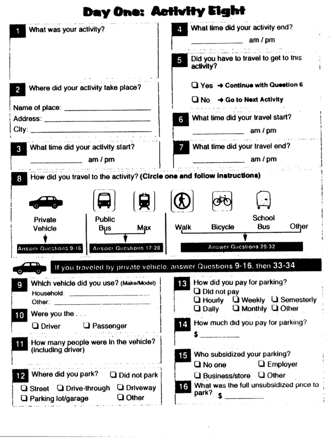
Figure 5.1(a) Portland activity and travel diary form, page 1...80
Figure 5.1(b) Portland activity and travel diary form, page 2...81
Figure 5.2 Portland day activity schedule model system ...83
Figure 5.3 Estimated disutility of generalized time in the tour models...91
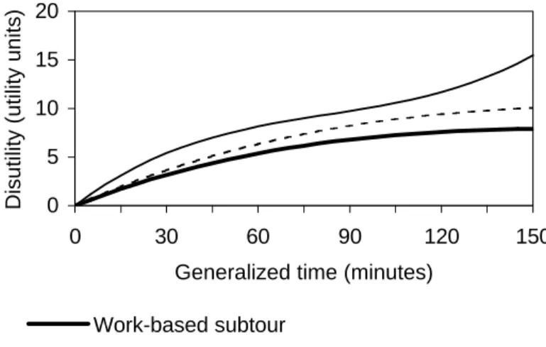
Figure 5.4 Estimated disutility of generalized time in subtours and intermediate stops...96
Figure 5.5 Suggested table format for collecting transportation information in the diary ...135
Figure 6.1 Model application ...138
Tables
Table 1.1 Model and variable types in the Portland day activity schedule model system... 24
Table 1.2 Peak period toll--induced leisure travel captured by the day activity schedule model ... 26
Table 2.1 An estimate of the number of day activity schedule alternatives faced by an individual ... 42
Table 2.2 Behavior-theoretical requirements of the activity-based travel demand forecasting model ... 44
Table 3.1 Requirements of the activity-based travel demand forecasting model ... 46
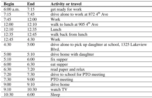
Table 4.1 Hypothetical example--activity and travel diary ... 68
Table 4.2 Hypothetical example—day activity pattern attributes ... 68
Table 4.3 Hypothetical example—tour attributes ... 68
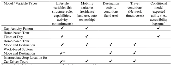
Table 5.1 Model and variable types in the Portland day activity schedule model system... 84
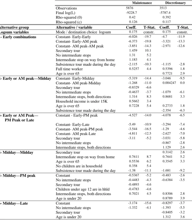
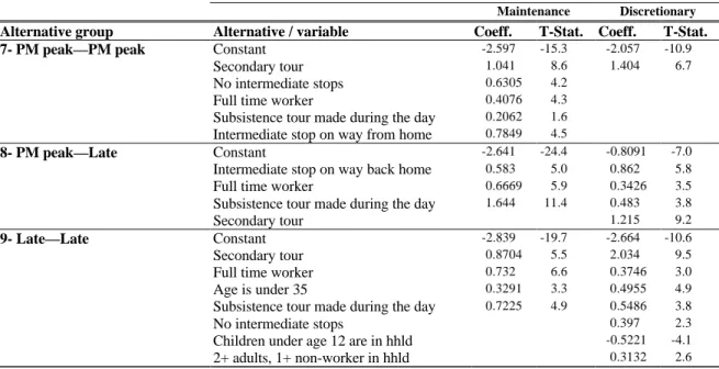
Table 5.3 Home-based non-work tour times of day choice models... 88
Table 5.4 Values of time estimated from stated preference data ... 91
Table 5.5 Home-based tour mode/destination choice models ... 92
Table 5.6 Work-based tour mode/destination choice model... 94
Table 5.7 Intermediate activity location choice models for car driver tours... 95
Table 5.8 Day activity pattern choice dimensions and choice set for each dimension... 97
Table 5.9 Sample pattern distribution by primary activity, at-home vs on-tour and primary tour type... 98
Table 5.10 Sample pattern distribution by primary activity and number & purpose of secondary tours... 99
Table 5.11 Sample pattern distribution by primary activity and at-home maintenance participation ... 98
Table 5.12 Lifestyle and mobility variables in the Portland day activity pattern utility functions...104
Table 5.13 Distribution of the sample patterns, classified by variables in the model ...105
Table 5.14 Summary statistics from day activity pattern model estimation...106
Table 5.15 Day activity pattern model—number of parameters by utility component and variable type...107
Table 5.16 Benchmark variable values for evaluating scale of utility function ...107
Table 5.17 Primary subsistence activity lifestyle variables...109
Table 5.18 Primary maintenance activity lifestyle variables...110
Table 5.19 Primary leisure activity lifestyle variables...112
Table 5.20 Secondary on-tour maintenance activity lifestyle variables ...113
Table 5.21 Secondary at-home maintenance activity lifestyle variables ...114
Table 5.22 Secondary on-tour leisure activity lifestyle variables ...115
Table 5.23 Placement of secondary maintenance and leisure activities in subsistence patterns...118
Table 5.24 Placement of secondary maintenance and leisure activities in maintenance patterns...119
Table 5.25 Placement of secondary maintenance and leisure activities in leisure patterns...120
Table 5.26 Secondary activity combinations on primary tour ...121
Table 5.27 Subsistence pattern inter-tour combinations ...122
Table 5.28 Maintenance pattern inter-tour combinations...123
Table 5.29 Leisure pattern inter-tour combinations ...123
Table 5.30 Tour accessibility logsums ...125
Table 5.31 Statistical tests of pattern model restrictions ...126
Table 5.32 Suggested activity categories for the activity diary ...134
Table 6.1 Day activity pattern adjustments for $.50 per mile peak period toll...143
Table 6.2 Half-tour predictions under the $.50 per mile peak period toll...145
Table 6.3 Predicted toll response of 22 population segments—primary activity purpose...147
Table 6.4 Predicted toll response of 22 population segments—primary tour type ...149
Table 6.5 Predicted toll response of 22 population segments—secondary tours and at-home maintenance .150 Table 6.6 Pattern adjustments for transit access improvement and auto ownership restriction ...151
Table 6.7 Half-tour predictions for transit access improvement and auto ownership restriction ...152
Introduction and Summary
1.1 Introduction
This thesis presents a model of the individual’s activity and travel scheduling decision that can be used like traditional models for urban travel forecasting and analysis. The work is motivated by the well-established notion that travel demand is derived from the demand for activities. It should therefore be modeled as a component of an activity scheduling decision, and models that fail to do this suffer from misspecification that may substantially undermine their ability to forecast. The second motivation is that, although much research has aimed at improving our conceptual understanding of this phenomenon or developing advanced models for capturing certain components of activity scheduling behavior, few have developed
models complete and simple enough to be used for general purpose urban travel forecasting. Of these, none has done it with a scheduling decision that at least spans an entire day, perhaps the most important temporal unit for activity scheduling. Our objective is therefore to develop a model of a person’s day activity schedule—the schedule of activities and travel spanning a 24 hour day—that can be incorporated into urban forecasting model systems. We may subsequently refer to the day activity schedule as the activity schedule, or schedule, for short.
A hypothetical example provides an intuitive understanding of the need for a model that represents travel as a component of an activity scheduling decision. Figure 1.1(a) depicts a simplified representation of a person’s day activity schedule, showing it as a continuous path in time and space. This person spends time at home in the morning, travels by auto to her workplace where she works throughout the day. In the late afternoon she heads for home in her car, but stops en-route at a familiar store to shop, then continues home where she remains
for the rest of the evening. Now suppose the state government decides to impose a peak period toll on the highways in this person’s commute path, substantially increasing her commute costs. How might she respond? If she is time sensitive she may breathe a sigh of relief and continue her schedule as is, happy to pay the extra cost in exchange for a faster commute. If she is cost sensitive and has good transit connections between home and work she may change modes for her commute (Figure 1.1(b)). However, if the transit line does not stop near her desired shopping location or she is uncomfortable carrying packages on the transit vehicle, she may come straight home on her commute and either walk or drive to a store after arriving home, depending on whether her neighborhood has walk-accessible shops. Alternatively, she may decide it is time to start planning her shopping activity more carefully and include the shopping stop only occasionally in her schedule. If she lacks good transit connections, but has flexible work hours she may continue using her car, but work earlier in the day and do her shopping on a separate tour1 to avoid the peak period tolls (Figure 1.1(c)). Or, she might decide to start working four ten-hour days, pay the peak period toll in the afternoons, and shop during the day on her extra day off. She may have the freedom to begin working at home some days, and do her shopping in the middle of the day (Figure 1.1(d)).
These are only some of the likely responses a person may make to a single policy initiative. They include changes in destination, timing and mode, which we refer to as the travel components of the schedule. They also include activity participation adjustment, changes in the number of tours, and trade-offs between at-home and on-tour activity locations. These attributes of the schedule we refer to as the activity pattern2 , since they define the
configuration, or pattern, of the day’s activities. In each case, changes in the travel components are linked closely with changes in the activity pattern. Persons with different lifestyles and resulting activity objectives, such as the need to get children to and from day care providers, might choose from a substantially different set of schedule alternatives.
1
We define a tour as a journey beginning and ending at the same location. This location is the base of the tour. Thus a journey beginning and ending at home is called a home-based tour. We refer to a work-based tour as a subtour, since it occurs in the midst of a home-based tour.
2
We also refer to the activity pattern as the day activity pattern or as the pattern. The day activity schedule model we subsequently develop explicitly represents the day activity pattern, and formally defines its attributes.
Other changes in activity and travel conditions, such as infrastructure changes, vehicle or fuel taxes, parking fees or regulation, telecommute or transit incentive programs, and traffic management could induce a similar variety of complex schedule adjustments involving travel components and the activity pattern.
Work Shop
Space
Time
(c) Time & pattern changes
Work Shop Space Time (d) Work at home Space Time Work Space Time Shop Auto Transit Shop
(b) Mode & pattern changes (a) Activity and travel schedule
Work
Work
Figure 1.1 Activity schedule adjustments to a peak period toll
(a) The schedule prior to the toll includes travel by auto to work, with a shopping stop on the homebound commute. Possible responses to a peak period toll (shown shaded in gray) include (a) no change, (b) a mode change to avoid the toll, (c) a time shift to avoid the toll, and (d) work at home. In cases (b) through (d), the adjustment also involves a pattern change, either the splitting of the shopping activity into a separate tour, or the shift from on-tour work to at-home work.
1.2 Summary
1.2.1 Theory of activity-based travel demand
The literature establishes our objective of modeling travel demand as part of the activity scheduling decision, of which it is a component. The scheduling decision is motivated by the individual’s desire to satisfy personal needs through activity participation, with at least a desire or tendency toward maximizing some objective related to this needs satisfaction (Ben-Akiva and Bowman, 1998). Great heterogeneity of needs exists among people, correlated with observable household and personal characteristics (Jones, Dix, Clarke et al., 1983). People face constraints that limit their activity schedule choice. Notably, activities are sequentially connected in a continuous domain of time and space, and are interrupted on a daily basis for a major period of rest. Travel occurs primarily to achieve activity objectives in the presence of these constraints (Hagerstrand, 1970).
Activity and travel scheduling occurs within a broader framework of interacting household decisions and urban processes (Ben-Akiva, 1973; Ben-Akiva and Lerman, 1985; Ben-Akiva, Bowman and Gopinath, 1996). From the standpoint of our desire to model activity and travel scheduling, four characteristics of the decision framework are most important. First, the scheduling decision is conditioned by the outcomes of longer term processes, including the household’s lifestyle and mobility outcomes, as well as the activity opportunity outcomes of the urban development process. Second, and closely related to the first, the scheduling process is not temporally sequential, but is governed by commitments and priorities, within the constraints of a given scheduling time period. Third, a one-day schedule period is natural because of the daily rest period’s regulating effect, but scheduling interactions occur over even longer time periods. Fourth, the scheduling process interacts with the performance of the transportation system; the demand resulting from the aggregation of all individuals’ scheduling choices determines system performance, and the scheduling decisions are influenced by perceptions of that system performance.
The biggest problem facing the activity schedule modeler is the immense number of schedule alternatives from which the activity scheduler may choose; the scheduling decision involves
the selection of activity purpose, sequence, timing, location, mode and route for many inter-related activities. The process can be viewed as comprising two stages: choice set
generation—the search for alternatives—and the choice of one alternative from the choice set3. Within this basic structure many alternative assumptions can be made about the nature of the process. The most frequently assumed protocol for modeling decisions is that of utility maximization from an exhaustively determined feasible set of alternatives. This is not
realistic in the context of such a large set of alternatives, but successful methods of
implementing alternative protocols for choice problems approaching this size have not been developed.
The review of activity-based travel behavior theory has sharpened the modeling objective. We aim to model travel demand decisions as components of a day activity schedule,
including the interacting dimensions of activity purpose, priority, timing, location, and travel mode. The model should be conditioned on longer-term urban processes, and household lifestyle and mobility outcomes, and interact with processes that determine transportation system performance attributes. Finally, the model needs to be tractable and accurately represent the scheduler’s need to simplify a decision that has countless feasible outcomes.
1.2.2 Models of activity and travel scheduling
We supplement the behavior-theoretical requirements to assure the development of a model that is technically sound, has adequate detail to be sensitive to relevant policies, has practical resource requirements for implementation and use, and produces valid forecasts.
Given the modeling requirements, a review of approaches that have been used in attempts to make activity-based travel forecasting practical leads to the modeling approach taken in this research, a nested system of discrete choice models. Markov and semi-Markov approaches represent the scheduling decision as a sequence of transitions, following the temporal
sequence of the day, with transitions between states corresponding to trips between activities. Their fundamental weakness is their basis in a decision sequence tied to the temporal activity
3
For a general discussion of the choice process, including definitions of choice set (the alternatives considered), universal set (the feasible alternatives), choice set generation and other terms, see Section 2.4 .
sequence, rendering them unable to adequately represent a decision process that is governed more by commitments and priorities than by sequence.
Rule-based models, reviewed in Section 3.3 , simulate schedule outcomes, employing a complex search rule accompanied by a simpler choice model, frequently with iteration occurring between search and choice. These systems are based on various decision theories, such as cognitive limitation or the notion of a search that terminates with acceptance of a satisfactory alternative. Existing rule-based simulations face two important challenges. First, they rely on a detailed exogenous activity program or schedule that determines all or much of the activity participation decision, as well as other important attributes such as location and timing. Thus, although the resulting schedules may be fairly complete in scope, important major components of the schedule are not modeled. Second, they rely on
unproven search heuristics and their decision protocols can be extremely complex. Extensive data and validation requirements accompany their complexity. Although rule-based
simulations are attractive because of the freedom they give to attempt new and potentially improved decision protocols, the accompanying challenges make them unlikely to yield a comprehensive, validated scheduling model in the near future.
In contrast, utility maximization, usually employed in tandem with simple deterministic choice set generation by econometric model systems, is a much simpler protocol for which the schedule scope is a less formidable modeling challenge. The protocol has a solid basis in consumer theory. Although its use of a large choice set pushes it beyond the limits of purely representing rational consumer behavior, the protocol has been successfully used and
validated in discrete choice travel demand model systems where the size of the choice set exceeds the number a person can rationally consider.
Econometric models, systems of equations representing probabilities of decision outcomes, can be viewed in two subclasses, discrete and mixed discrete-continuous. Discrete choice models partition the activity schedule outcome space into discrete alternatives. They deal with the big universal set by subdividing decision outcomes and aggregating alternatives. For example, the simplest models subdivide outcomes by modeling trip decisions instead of an entire day’s schedule, and aggregate activity locations into geographic zones.
Mixed discrete-continuous models focus attention on the continuous time dimension of the activity schedule, seeking to improve on its traditionally missing or weak aggregate
representation in discrete choice models. They combine continuous duration models with discrete choice models for other dimensions of the schedule. However, they have not yet expanded in scope to include most dimensions of the activity schedule, nor have they incorporated duration sensitivity to time-variant activity and travel conditions. Their use in models satisfying the requirements we have identified awaits further methodological development.
1.2.3 Discrete choice modeling approaches
Over time, discrete choice modelers have tried to improve behavioral realism by including more and more dimensions of choice in an integrated system matching the natural hierarchy of the decision process. Lower dimensions of the scheduling hierarchy are conditioned by the outcomes of the higher dimensions. For example, choice of travel mode for the work commute is conditioned by choice of workplace. At the same time the utility of a higher dimension alternative depends on the expected utility4 arising from the conditional dimension's alternatives. In our example, the choice of workplace is influenced by the expected utility of travel arising from all the available commute modes.
Nested logit models effectively model multidimensional choice processes where a natural hierarchy exists in the decision process, using conditionality and expected utility as described above. The expected utility of the conditional dimension is commonly referred to as
accessibility because it measures how accessible an upper dimension alternative is to opportunities for utility in the lower dimension. It is also often referred to as the "logsum", because in nested logit models it is computed as the logarithm of the sum of the
exponentiated utility among the available lower dimension alternatives (Ben-Akiva and Lerman, 1985, Chapter 10).
4
The utility arising from the conditional dimension’s alternatives is the maximum utility among the alternatives. This is a random variable, and its expected value is the expected utility referred to here, sometimes also referred to as expected maximum utility.
The models are disaggregate, representing the behavior of a single decisionmaker. A Monte-Carlo procedure is often used to produce aggregate predictions. In other words, the models make predictions with disaggregate data, requiring the generation of a representative population. The model is applied to each decisionmaker in the population—or a representative sample—yielding either a simulated daily travel itinerary or a set of probabilities for alternatives in the choice set. The trips in the itinerary can then be aggregated and assigned to the transport network, resulting in a prediction of transport system performance. This process may require replications to achieve statistically reliable predictions.
The simplest and oldest subclass of discrete choice model systems divides the activity schedule into trips5. One of the earliest of the integrated trip-based systems, developed for the Metropolitan Transportation Commission (MTC) of the San Francisco Bay area is reviewed in Section 3.4.3 (Ruiter and Ben-Akiva, 1978). More recently, models have been developed that combine trips explicitly in tours, including the Stockholm model system reviewed in Section 3.4.4 (Algers, Daly, Kjellman et al., 1995).
The main behavioral criticism of the trip- and tour-based discrete choice model systems is the division of the schedule outcome into separate pieces—trips or tours—and the failure to represent at-home activity participation. Otherwise, they satisfy the identified theoretical and practical requirements. Although their practicality is closely tied to their undesirable division of the schedule into pieces, advances in computing technology make further integration of the schedule representation an attractive possibility. Thus, we choose the discrete choice approach.
1.2.4 The day activity schedule model system
The day activity schedule is viewed as a set of tours and at-home activity episodes tied together by an overarching day activity pattern, or pattern for short (Figure 1.2). Decisions about a specific tour in the schedule are conditioned by the choice of day activity pattern.
5
A trip is defined as the journey from one activity location to the next. It may involve travel by more than one mode.
This is based on the notion that some decisions about the basic agenda and pattern of the day’s activities take precedence over details of the travel decisions. The probability of a particular day activity schedule is therefore expressed in the model as the product of a marginal pattern probability and a conditional tours probability
p schedule( )= p pattern p tours pattern( ) ( | )
where the pattern probability is the probability of a particular day activity pattern and the conditional probability is the probability of a particular set of tours, given the choice of pattern.
Day Activity Schedule
Day Activity Pattern
Tours
Figure 1.2 The day activity schedule
An individual’s multidimensional choice of a day’s activities and travel consists of tours interrelated in a day activity pattern.
The day activity pattern represents the basic decisions of activity participation and priorities, and places each activity in a configuration of tours and at-home episodes. Each pattern alternative is defined by (a) the primary activity of the day, (b) whether the primary activity occurs at home or away, (c) the type of tour for the primary activity, including the number, purpose and sequence of activity stops, (d) the number and purpose of secondary tours, and (e) purpose-specific participation in at-home activities. For each tour, details of time of day,
destination and mode are represented in the conditional tour models. Within each tour, the choice of timing, mode and primary destination condition the choices of secondary stop locations.
We assume the utility of a pattern includes additively a component for each activity, a component for the overall pattern, and a component for the expected utility of its tours. The activity components can capture basic differences among people in the value of various kinds of activity participation. The pattern component captures the effect of time and space
constraints in a 24-hour day. The expected utility component captures the effect of tour conditions on pattern choice. Through it the relative attractiveness—or utility—of each pattern, depends not just directly on attributes of the pattern itself, but also on the maximum utility to be gained from its associated tours. Patterns are attractive if their expected tour utility is high, reflecting, for example, low travel times and costs. This ability to capture sensitivity of pattern choice—including inter-tour and at-home vs on-tour trade-offs—to spatial characteristics and transportation system level of service distinguishes the day activity schedule model from tour models, and is its most important feature.
The day activity schedule model also improves on tour models’ ability to represent the time dimension by explicitly modeling the time of each one of the inter-related tours in the
pattern. With these features, the day activity schedule model satisfies the identified behavior-theoretical requirements.
1.2.5 The Portland day activity schedule model system
The empirical implementation for Portland, Oregon, tests the feasibility of achieving the requirements for a practical forecasting system without compromising the theoretical requirements. Secondly it tests the importance of the integrated day activity schedule representation; is there evidence that the extra cost and complexity yield improvements in model performance?
We adopt a structure in which tours are assumed to be conditionally independent, given the pattern choice. For home-based tours, tour timing conditions the joint choice of tour mode and destination. Work-based subtours are modeled conditional on the work tour, and these
condition any stops occurring before or after the primary activity. At each conditional level, the probability is represented by a multinomial logit model.
Figure 1.3 shows the overall structure of the activity-based model system. Lower level choices are conditioned by decisions modeled at the higher level, and higher level decisions are informed from the lower level through expected maximum utility variables.
Day Activity Pattern
Home based tours times of day
Home based tours mode and destination
work-based subtours
Intermediate stop locations for car driver tours
INPUT households zonal data network data OUTPUT OD Trip matrices by mode, purpose, time of day and income class Pattern (and
associated tour) probabilities
Expected tour time-of day utilities
Tour time-of-day probabilities
Expected tour mode and destination utilities
Tour mode and destination probabilities
Expected subtour and intermediate stop utilities (not in current implementation)
Figure 1.3 Portland day activity schedule model system
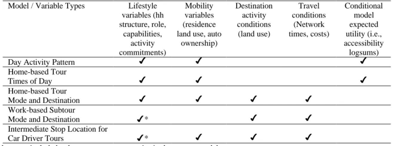
Table 1.1 shows the five main types of models included in the system, as well as the types of variables included in each of the model types. The variables include important lifestyle categories and mobility decisions, attributes of the activity and travel environment, and the expected utility variables from the conditional models. The entire system includes 633 estimated parameters, including 297 measuring the importance of lifestyle and mobility variables, 95 measuring the importance of the activity and travel environment—including
expected utility, and 241 measuring unexplained preferences and the influence of marginal choice dimensions on conditional dimension utility.
Table 1.1 Model and variable types in the Portland day activity schedule model system
Model / Variable Types Lifestyle variables (hh structure, role, capabilities, activity commitments) Mobility variables (residence land use, auto
ownership) Destination activity conditions (land use) Travel conditions (Network times, costs) Conditional model expected utility (i.e., accessibility logsums)
Day Activity Pattern 4 4 4
Home-based Tour
Times of Day 4 4 4
Home-based Tour
Mode and Destination 4 4 4 4
Work-based Subtour
Mode and Destination 4* 4 4
Intermediate Stop Location for
Car Driver Tours 4* 4 4 4
*these are included only as aggregate categories in the current model system
As implemented, the home-based tour predictions are aggregated into zone-to-zone counts of half-tours6 for each of several income classes. The work-based subtour and intermediate stop7 models are applied to these counts, using aggregate categorical variables, and do not supply the upper level models with measures of expected maximum utility. This design compromise substantially reduces the time required to apply the model in a production setting, making it feasible to apply the entire model system using 300mhz Pentium-based microcomputers. This compromise should be eliminated in subsequent production implementations of the model system as advances in computing technology allow. As discussed in Chapter 6, it makes the pattern model insensitive to differential effects of travel conditions on patterns with different numbers of secondary stops.
In the day activity pattern model, likelihood ratio tests were conducted to test the collective significance of groups of variables in the pattern model. The tests support the importance of variables in the four lifestyle categories used in the model: household structure, role in household, personal and financial capabilities, and activity commitments. They support the
6
A half-tour is either portion of a tour between the origin and the primary destination. It includes more than one trip if activities occur between the origin and primary destination.
7
An intermediate stop is a stop for activity during a half-tour. Each intermediate stop adds a trip to the half-tour.
importance of the secondary at-home maintenance activity parameters in subsistence and leisure patterns, indicating that the identification of secondary at-home maintenance is important in the pattern choice set definition8. The tests also indicate that it is important in the choice set definition to distinguish the placement of secondary activities on the pattern in several ways: (a) whether they occur on the primary tour or a separate tour, (b) relative to the primary activity in the primary tour, and (c) specific to pattern purpose and secondary
activity purpose. Finally, a test supports the importance of the tour expected maximum utility parameters as a group. This is an important result in light of the major hypothesis of this study that it is important to represent travel demand in the context of the day activity schedule. With these expected maximum utility variables, changes in tour utility, caused by changes in the transport system performance or in spatial activity opportunities, have a significant effect on the choice of pattern. Such effects cannot be captured by tour or trip-based travel demand models. Testing of the pattern model’s multinomial logit assumption remains as a future objective. The need probably exists for nesting, and perhaps more complex correlation structures, because of the multidimensional nature of the pattern choice. For example, strong random utility correlation probably exists among patterns that share primary purpose. Nevertheless, the tests conducted provide strong evidence, in addition to the individual parameter tests of the previous sections, in support of the basic model structure, utility function structure and lifestyle variable categories of the day activity schedule model.
1.2.6 Model application and evaluation
The model system demonstrates the benefits of its design in various policy applications, including peak period pricing. There, in response to a toll levied on all travel paths during the morning and evening peak travel periods, the model predicts not only shifts in travel
8
Pas (1982), adopting the approach of Reichman (1976), places all out-of-home activities in the three broad categories of subsistence, maintenance and leisure. He defines work and school as
subsistence, and shopping and personal business as maintenance. We adopt these categories for in-home activities as well, defining subsistence as activity, including education, devoted to the current or future generation of household income, maintenance as non-income-generating activities
required to maintain a household, and leisure as optional activities engaged in for enjoyment. We also use the term discretionary interchangeably with leisure.
mode and timing, but also shifts in pattern purpose and structure. As shown in Table 1.2, the net result is an increase in the predicted number of tours for leisure purposes; increases in leisure tours induced by pattern changes more than offset leisure tour decreases caused by the peak period toll.
Table 1.2 Peak period toll--induced leisure travel captured by the day activity schedule model Percent change in number of tours, by tour purpose, in response to $.50 per mile
peak period toll on all roads Time of day Work Maintenance Leisure A.M. peak period -7.1% -8.4% -6.2% P.M. peak period -7.4 -7.7 -1.5
Midday 3.1 3.6 2.8
Outside peaks 6.8 2.3 2.7
Total -2.5% -0.3% +.8%
How does the model capture this induced demand? Increased peak period travel costs reduce expected maximum mode/destination utility (logsums) in the peak period alternatives of the times-of-day choice models, and expected maximum time of day utility in the pattern choice model, where patterns with tours that rely most heavily on peak period auto travel become relatively less attractive. Thus, there is a shift away from patterns with subsistence tours in the pattern model, toward all other pattern types. The net change in maintenance and leisure tours could be positive or negative, because the increase in number of maintenance and leisure patterns, and the introduction of secondary tours on changed patterns, tend to offset the pattern simplification effect for these purposes. In the example, the model actually predicts a net increase in leisure tours.
The above explanation of model response to the peak period tolls excludes the impact on intermediate stop location models and work-based tours. These too are affected by the peak period tolls, through the toll’s direct effect on stop utility, as well as pattern changes and tour destination changes. However, by omitting the expected utility connection of intermediate stops to home-based tours, the model system underestimates the toll’s tendency to reduce trip chaining during the peak period.
The previous analysis ignores the lifestyle effects in schedule choice and the associated potential heterogeneity of response to the toll policy. Predicted pattern shifts are analyzed in each of four activity pattern dimensions—primary activity purpose, primary tour type, secondary tours, and at-home maintenance activity—for 22 population segments, defined by household structure and role, capabilities, activity commitments and mobility decisions. The model captures much heterogeneity in pattern choice and in response to the toll policy, clearly demonstrating the importance of explicitly modeling heterogeneity in the pattern choice.
Analysis of model response to additional policies, including transit improvements, vehicle ownership restrictions, fuel taxes, auto registration fees, parking regulation, neighborhood walkability improvements, mixed use development, and ITS highway capacity increases, and telecommunications advances indicate that the day activity schedule model structure enables the capture of pattern shifts and associated changes in travel demand in a great variety of situations. However, in some cases, the implemented model’s sensitivity to the policy would be limited because of coarse resolution of schedule dimensions or because of missing
variables in the specification. For one example, coarse spatial resolution limits the model’s ability to capture the effect of walkability improvements. For another example, the model lacks variables such as the possession of a credit card or a home computer with modem, that if included might enable it to capture pattern changes caused by improvements in information technology.
1.2.7 Conclusions
The overall conclusion of this study is that a travel forecasting model system based on a discrete choice model of the day activity schedule is practical and captures anticipated activity pattern shifting, with associated travel changes, that previous models have missed.
The day activity schedule model, specified in Chapter 4, satisfies a rich set of requirements derived from the literature on activity-based travel demand, providing the foundation for the development of behaviorally improved travel demand forecasting models. Its full-day scope; detail of pattern, activity and travel dimensions; and integrated structure give the model
design three important realistic performance capabilities. First, it can capture the trade-offs people consider as they face time and space constraints in scheduling their day’s activities. These include variations in activity participation, on-tour versus at-home activity location, number of tours, trip chaining, timing, destination and travel mode. Second, it can
realistically capture the significant influence of lifestyle-based heterogeneity on schedule choice by identifying lifestyle and mobility factors in each of the model’s many scheduling dimensions. Third, it can capture the impact of exogenous factors upon all dimensions of schedule choice, even if the factors only act directly in one dimension. Importantly, this includes the influence of activity accessibility—including travel conditions—on the choice of activity pattern.
The empirical implementation has shown that, though compromises were made in the representation of the activity schedule to enable practical use of the approach, it can handle the scope of the activity schedule at a level of detail matching or exceeding trip or tour-based systems. The model system demonstrates the benefits of its design in various policy
applications, such as peak period pricing, capturing pattern shifts and resulting travel demand effects that trip and tour-based models cannot capture.
1.2.8 Research topics
This study creates many opportunities for fruitful research and development, to verify and exploit the benefits of the day activity schedule approach in travel forecasting, to enhance it by addressing unresolved issues, and to integrate it with related models of household choice, urban development and transport systems. It can also be evaluated for theoretical
weaknesses, serving as grist for the further development of theory and models of activity and travel behavior. Specific research topics include (a) model validation; (b) development of efficient, consistent application procedures with known confidence levels; (c) testing and enhancement of the day activity schedule model, including the 570 alternative pattern, integration of expected utility from secondary stops and subtours, generalized day activity pattern correlation structures, temporal and spatial resolution, secondary tours conditioned by primary tour outcomes, and conditioning of model on usual workplace and commute mode; (d) procedures to combine data from enhanced surveys; (e) schedule model enhancements
that require improved data sets, including improved activity purpose resolution,
telecommunications effects, effects of unusual transportation conditions, and heterogeneity; (f) techniques to improve computational efficiency and incorporate alternative decision protocols; (g) integration of activity and mobility models, using expected schedule utility to explain mobility choices; and (h) reconciliation of the day activity schedule model
specification with formal theories of transport economics and home production economics.
1.2.9 Outline of the thesis
In Chapter 2, the theory of activity-based travel demand is examined, resulting in a set of behavior-theoretical requirements for an activity-based travel demand model system based on a day activity schedule. Chapter 3 studies previous attempts to model travel demand as part of a larger activity schedule, leading to the selection of the discrete choice modeling
approach. Chapter 4 presents the concepts and mathematical form of the day activity schedule model, and identifies important model design issues. Chapters 5 and 6 present the results of an empirical implementation in Portland, Oregon, that (a) demonstrates the practical feasibility a day activity schedule model system satisfying the behavioral requirements of Chapter 2, and (b) tests the importance of the day activity schedule representation. Chapter 7 draws the final conclusions of the thesis and discusses specific ideas for future research to build on those conclusions.
Theory of Activity-based Travel Demand
In the first section of this chapter an examination of the literature establishes our objective of modeling travel demand as part of the activity scheduling decision. Given this objective, we place the activity scheduling decision in a broader decision framework, then consider how activity scheduling is affected by longer term lifestyle decisions and outcomes, and face the principal challenge of modeling activity scheduling behavior, namely the immense set of alternatives from which the activity schedule is chosen. This leads to a set of theoretical requirements for the development of an activity-based travel demand model.
2.1 The characteristics of activity and travel demand
One of the most fundamental and well-known principles is that travel demand is derived from activity demand. This principle implies a decision framework in which travel decisions are components of a broader activity scheduling decision, and calls for modeling activity demand. Chapin (1974) theorized that activity demand is motivated by basic human desires, such as survival, social encounters and ego gratification. Activity demand is also moderated by various factors, including, for example, commitments, capabilities and health.
Unfortunately, it is difficult to model the factors underlying this demand, and little progress has been made in incorporating the factors in travel demand models. However, a significant amount of research has been conducted on how household characteristics moderate activity demand. This research concludes that (a) households influence activity decisions, (b) the effects differ by household type, size, member relationships, age, gender and employment status and (c) children, in particular, impose significant demands and constraints on others in the household (Chapin, 1974; Jones, Dix, Clarke et al., 1983; Pas, 1984).
Hagerstrand (1970) focused attention on constraints--among them coupling, authority, and capability--which limit the individual's available activity options. Coupling constraints require the presence of another person or some other resource in order to participate in the activity. Examples include participation in joint household activities or in those that require an automobile for access. Authority constraints are institutionally imposed restrictions, such as office or store hours, and regulations such as noise restrictions. Capability constraints are imposed by the limits of nature or technology. One very important example is the nearly universal human need to return daily to a home base for rest and personal maintenance. Another example Hagerstrand called the time-space prism: we live in a time-space continuum and can only function in different locations at different points in time by experiencing the time and cost of movement between the locations.
The concepts of activity-based demand, and time and space constraints, have also been incorporated in the classical model of the budget-constrained utility-maximizing consumer. Becker (1965) made utility a function of the consumption of commodities that require the purchase of goods and the expenditure of time. DeSerpa (1971) explicitly identified the existence of minimum time requirements for consumption of goods. Evans (1972)
generalized the model, making utility a function only of activity participation; formulating a budget constraint based on a transformation which relates the time spent on activities, the goods used in those activities and the associated flow of money; and introducing coupling constraints which, among other things, allow the explicit linking of transportation
requirements to the participation in activities. Jara-Diaz (1994) extended an Evans type model explicitly to allow the purchase of goods at alternative locations, each associated with its own prices, travel times and travel costs, all of which enter the time and budget
constraints. He also included a transformation relating the purchase of goods to required trip-making. In maximizing utility, the consumer chooses how much time to spend on various activities, how many trips to make overall, what goods to buy and where, and the travel mode for each trip. These efforts to incorporate activities, time and space into the formal economic model of the consumer stop short of addressing important aspects of the scheduling problem, such as temporally linking activities or allowing for the chaining of trips between activity locations.
A substantial amount of analysis has been done to refine the notion of activity-based travel demand, test specific behavioral hypotheses, and explore modeling methods. We present here only a few highlights. Pas and Koppelman (1987) examine day-to-day variations in travel patterns, and Pas (1988) and Hirsch, et al (1986) explore the representation of activity and travel choices in weekly activity patterns. Kitamura (1984) identifies the interdependence of destination choices in trip chains. Kitamura, et al (1995) develop a time- and distance-based measure of activity utility that contrasts with the typical travel disutility measure. Hamed and Mannering (1993) and Bhat (1996b) explore methods of modeling activity duration. Bhat and Koppelman (1993) propose a framework of activity agenda generation.
For extensive summaries of other results, and access to reading lists, the interested reader can examine one or more of the published reviews of this literature. Damm (1983) compiles a list of empirical research, categorizes the hypotheses tested, lists the explanatory variables associated with each class of hypothesis, and presents the statistical results of parameter estimates. Golob and Golob (1983) examine the literature by categorizing 361 works by primary and secondary focus, with the five focus categories being activities, attitudes, segmentations, experiments, and choices. Kitamura (1988) updates the review, categorizing works by the topics of activity participation and scheduling, constraints, interaction in travel decisions, household structure and roles, dynamic aspects, policy applications, activity models and methodological developments. Perhaps the best recent review of the theoretical contributions in activity-based travel demand analysis is that of Ettema (1996) who describes contributions from the fields of geography, urban planning, microeconomics and cognitive science.
In summary, the literature establishes our objective of modeling travel demand as part of the activity scheduling decision, of which it is a component. The scheduling decision is
motivated by the individual’s desire to satisfy personal needs through activity participation, with at least a desire or tendency toward maximizing some objective related to this needs satisfaction. Great heterogeneity of needs exists among people, correlated with observable household and personal characteristics. People face constraints that limit their activity schedule choice. Notably, activities are sequentially connected in a continuous domain of time and space, and are interrupted on a daily basis for a major period of rest.
We next examine the context of the activity and travel scheduling decision.
2.2 Activity and travel decision framework
Figure 2.1 shows how activity and travel scheduling decisions are made in the context of a broader framework. They are part of a set of decisions made by a household and its
individual members, and in that context they interact with the urban development process and the performance of the transportation system. (Ben-Akiva, 1973; Ben-Akiva and Lerman, 1985; Ben-Akiva, Bowman and Gopinath, 1996).
Mobility and Lifestyle
(work, residence, auto ownership, activities, etc.) Urban Development
Activity and Travel Scheduling
(sequence, location, mode, etc.)
Implementation and Rescheduling
(route, speed, parking, etc.)
Transportation System Performance Household Decisions
Figure 2.1 Activity and travel decision framework
Many household decisions, occurring over a broad range of timeframes, interact with each other and with the urban development process and transportation system performance.
In the figure, the urban development box represents decisions of governments, real estate developers and other businesses. Governments may invest in infrastructure, provide services, and tax and regulate the behavior of individuals and businesses. Real estate developers provide the locations for residential housing and businesses. Where a firm chooses to locate, and its production decisions, affect job opportunities in that area. This conditioning of
individual behavior by urban development outcomes is represented in the figure by the downward pointing arrow joining the urban development and household decision boxes. The corresponding upward pointing arrow represents the fact that household decisions, such as residential choice, also influence urban development decisions. Taken together, the two arrows represent the interplay of household and urban development decisions in markets, such as real estate and employment, that establish conditions under which individual households and developers must operate.
Urban development and household decisions affect performance of the transportation system, such as travel volume, speed, congestion and environmental impact. At the same time, transportation system performance affects urban development and individual decisions.
Household and individual choices, including (a) lifestyle and mobility decisions, (b) activity and travel scheduling, and (c) implementation and rescheduling, fall into distinct time frames of decision making. Lifestyle and mobility decisions occur at irregular and infrequent intervals, in a time frame of years. Activity and travel scheduling occurs at more frequent and regular intervals. Unplanned implementation and rescheduling decisions occur within the day. Outcomes of the longer term processes condition the shorter term decisions, and are influenced by expected benefits associated with anticipated short term decisions.
We define lifestyle broadly, as a set of individual and household attributes, established as outcomes of major life decisions and events, and the gradual accumulation of minor changes, habits and preferences, that determines needs and preferences for activities, and the
resources available for their satisfaction. The lifestyle formation processes are strongly influenced by the accumulation of mobility, activity and travel outcomes. Lifestyle includes household structure (such as single adult, married couple with pre-school children or non-family adult group); individual role in the household (such as principal income earner or childcare giver); activity priorities, commitments and habits (such as absolute and relative devotion to job, property maintenance, hobbies, recreation and participation in civic, religious or social organizations); and financial and personal capabilities and limitations (such as wealth, income, vocational skills and physical disabilities).
Mobility outcomes are attributes, established by lifestyle-constrained decisions and events, that determine the availability and cost of access to activities. They are dominated by clearly defined choices occurring on an irregular and infrequent basis, but can also involve unchosen events such as a job transfer and emergent phenomena such as the gradual selection of a favorite shopping location. Although mobility decisions occur within a given lifestyle context, some of these decisions may be so major as to cause significant lifestyle changes. A mobility decision cannot be conditioned by the more frequent activity and travel decisions, but is influenced by expectations about the benefits to be gained from the activity and travel opportunities made possible by the choice, given the current lifestyle. Mobility decisions include location choices for work, residence, school and other repetitive activities determined by lifestyle; auto acquisition and other transportation arrangements; and arrangements for repetitive conduct of other activities by electronic or other non-travel means.
The activity and travel schedule is a set of activities conducted by a person over a continuous period of time, each activity characterized by purpose, priority, location, timing, and means of access. It is natural to view the schedule as spanning a one day time period because of the regulating effect of the overnight rest period. However, day-to-day interactions occur in scheduling decisions, so the schedule can also be viewed as having a longer time period. The schedule, although carried out by an individual, may be partly determined or influenced by the household. Alternatively, it can be viewed as a household schedule, including a set of activities for each member, and identifying activities in which members participate jointly.
The schedule is the outcome of two processes depicted by separate boxes in Figure 2.1, activity and travel scheduling , and implementation and rescheduling. Activity and travel scheduling yields a planned schedule. It is conditioned by the longer-term lifestyle and mobility outcomes. Given these constraints, and a scheduling period, the decisionmaker may freely arrange activities in various ways to best achieve activity objectives according to his or her priorities. Although the resulting schedule has a temporal sequence, the scheduling process is not temporally sequential. Instead, it is governed by commitments and activity priorities. Each component of the schedule is determined with basic knowledge of the other components of the schedule, and its placement is strongly conditioned by the placement of higher priority components of the schedule
Implementation and rescheduling yield an implemented schedule; during the scheduling period decisions are made to fill previously unscheduled time with unplanned activities, and rescheduling occurs in response to unexpected events. It can be viewed as the reiteration of the scheduling process, employing schedule adjustments at each step rather than replanning the entire schedule. The schedule adjustment decision is based on revised objectives and constraints, informed by the most recent events.
The framework presented here is consistent with the notions of Chapin, Hagerstrand and the activity-based consumer demand economists. Urban development and transportation system outcomes determine many of Hagerstrand’s constraints. Lifestyle and mobility decisions are conditioned by the same underlying factors that Chapin identified as motivating activity selection. They, along with urban development and transportation system outcomes determine many of Chapin’s moderating factors that also influence activity choice.
Likewise, they determine many of the time and space constraints incorporated in the activity-based consumer economists’ models of consumer behavior.
From the standpoint of our desire to model activity and travel scheduling, four characteristics of the decision framework are most important. First, the scheduling decision is conditioned by the outcomes of longer-term processes, including the household’s lifestyle and mobility outcomes, as well as the activity opportunity outcomes of the urban development process. Second, and closely related to the first, the scheduling process is not temporally sequential, but is governed by commitments and priorities, within the constraints of a given scheduling time period. Third, a one-day schedule period is natural because of the daily rest period’s regulating effect, but scheduling interactions occur over even longer time periods. Fourth, the scheduling process interacts with the performance of the transportation system; the demand resulting from the aggregation of all individuals’ scheduling choices determines system performance, and the scheduling decisions are influenced by perceptions of that system performance.