HAL Id: inserm-00861241
https://www.hal.inserm.fr/inserm-00861241
Submitted on 12 Sep 2013
HAL is a multi-disciplinary open access
archive for the deposit and dissemination of sci-entific research documents, whether they are pub-lished or not. The documents may come from teaching and research institutions in France or abroad, or from public or private research centers.
L’archive ouverte pluridisciplinaire HAL, est destinée au dépôt et à la diffusion de documents scientifiques de niveau recherche, publiés ou non, émanant des établissements d’enseignement et de recherche français ou étrangers, des laboratoires publics ou privés.
Per-subject characterization of bolus width in pulsed
arterial spin labeling using bolus turbo sampling.
Marjorie Villien, Emilie Chipon, Irène Troprès, Julien Bouvier, S. Cantin, D.
Chechin, Jean-François Le Bas, Alexandre Krainik, Jan Warnking
To cite this version:
Marjorie Villien, Emilie Chipon, Irène Troprès, Julien Bouvier, S. Cantin, et al.. Per-subject char-acterization of bolus width in pulsed arterial spin labeling using bolus turbo sampling.. Magnetic Resonance in Medicine, Wiley, 2013, 69 (6), pp.1677-82. �10.1002/mrm.24412�. �inserm-00861241�
Per-subject characterization of bolus width in Pulsed Arterial
Spin Labeling using Bolus Turbo Sampling (BoTuS)
M. Villien1,2, E. Chipon3, I. Troprès4, J. Bouvier1,2, S. Cantin5, D. Chechin6, J-F. Le Bas4,5, A. Krainik2,5, and J. M. Warnking1,2
1. INSERM, U836, Grenoble, France
2. Université Joseph Fourier, Grenoble Institut des Neurosciences, Grenoble, France 3. CHU de Grenoble, CIC – Innovation Technologique, Grenoble, France
4. Université Joseph Fourier, SFR1, Grenoble, France
5. CHU de Grenoble, Clinique Universitaire de Neuroradiologie et d’IRM, Grenoble, France 6. Philips Healthcare, Suresnes, France
Corresponding author: Jan Warnking
Grenoble Institut des Neurosciences
Centre de Recherche Inserm U 836 - UJF - CEA – CHU, Chemin Fortuné Ferrini Université Joseph Fourier - Site Santé, Bâtiment Edmond J. Safra
38706 La Tronche, France Tel: +33 04 56 52 05 85
Mail: jan.warnking@ujf-grenoble.fr
Word count: 2814
Abstract
Quantitative measurement of cerebral blood flow using QUIPSS II pulsed arterial spin labeling relies on the assumption that the time between label and QUIPSS saturation is shorter than the natural temporal bolus width. Yet, the duration of the bolus of tagged blood spins entering the region of interest may vary across subjects due to physiological differences in blood velocity or vessel geometry. We present a new technique, Bolus Turbo Sampling (BoTuS), to rapidly measure the duration of the inflowing bolus. This allows optimizing the ASL acquisition for each subject to ensure reliable quantification of perfusion while maximizing SNR by avoiding the use of unnecessarily short label durations. The repeatability of this technique is evaluated and its validity assessed by comparison with ASL data acquired at variable TI1 and by testing subjects at different physiologic states.
Introduction
Arterial Spin Labeling (ASL) is a quantitative MRI method to non-invasively measure cerebral blood flow (CBF)[1]. The longitudinal magnetization of water spins in arterial blood is inverted in the feedings arteries and subsequently the flowing tagged spins are imaged in the region of interest after a certain delay (TI2). ASL methods can be divided into continuous
and pulsed ASL (PASL) techniques depending on the way spins are tagged. PASL is widely used in clinical research protocols due to its ease of implementation, its lower specific absorption rate (SAR) and the absence of need for specific coils. The ASL signal depends not only on CBF but also on factors such as magnetization at equilibrium, tagging efficiency, temporal width of the bolus of tagged spins (2) and the transit time of blood from the label slab to the imaging slice[2]. The QUIPSSII[3] and Q2TIPS[4] sequences aim to eliminate sensitivity to bolus duration and transit times by saturating the longitudinal magnetization of labeled spins remaining in the label region after a delay TI1. This delay, if shorter than the
natural bolus duration, defines the temporal width of the bolus. However, if the saturation is applied too late, the actual temporal width of the bolus is shorter than TI1, leading to errors in
the quantification of CBF from the ASL signal[5].
One response to this issue are multi-TI ASL techniques like QUASAR[6] or Bolus-tracking ASL[7]. Since images are acquired at different inversion times, transit delay and bolus duration can be obtained and accounted for by fitting model functions to the ASL signal. However, multi-TI acquisitions require significantly longer acquisition times or limit the spatial coverage available, and require more sophisticated analysis techniques to obtain robust CBF maps.
Previous single-TI studies have tried to use optimal values for the saturation delay TI1, fixed
width and position of the label pulse implies that this optimization may need to be performed for each specific study[8]. Furthermore, if quantitative CBF measurements are to be guaranteed, the shortest natural bolus duration occurring in the patient population dictates the choice of the TI1 for all subjects, leading to a loss in sensitivity in subjects with longer label
durations.
The aim of this study is to validate a new technique (BoTuS, for Bolus Turbo Sampling) to measure the natural bolus duration 2 in each subject and thus to optimize the TI1 parameter
individually[9], [10]. This technique directly traces the bolus of the tagged spins for about three seconds after the application of the tag pulse, with a temporal resolution of fifty milliseconds. The initial shape of the bolus of the tagged spins is modeled as a boxcar function with flow through the vasculature modeled as a Gaussian dispersion of the tag in time[11], a modified version of the Hrabe-Lewis model[12], [13].
Methods
For this study, a total of thirteen healthy volunteers (age 23-40 years, five female) were scanned on a 3-T Philips Achieva TX whole body scanner using whole-body RF transmit and 8-channel head receive coils. The institutional review board approved the protocol and all subjects gave prior written consent to participate in the study. During all acquisitions we recorded physiological parameters of our subjects (EtCO2, SpO2, respiratory frequency, heart
rate) to verify that the subjects stayed in the same physiological state. The entire protocol consisted of two parts: 1) the measurement of the shape of the bolus using the BoTuS technique, performed twice under baseline physiologic conditions, once at the beginning and once towards the end of each session in order to assess repeatability, and performed once during globally increased CBF under hypercapnia at the end of the session 2) a different
measurement of the natural duration of the bolus from multi-TI1 data, to obtain an
independent measure of bolus width.
BoTuS protocol
The purpose of this part of the study was to assess the feasibility and the repeatability of the BoTuS technique. The aim of this sequence is to rapidly measure the bolus shape of the tagged spins entering our region of interest (ROI). The BoTuS sequence consists of a PICORE[3] tagging scheme (tag width=200 mm, label gap=15 mm) immediately followed by a rapidly repeated EPI read-out on one axial slice just above the Circle of Willis scanned every 50 ms until TI=2900 ms (Figure 1a). Acquisition parameters were: flip angle=90°, TE=19 ms, EPI BW=3525 Hz, voxel size=4*4*5 mm, NA=10 ctl-tag pairs, total scan duration=1’18”. The 90° flip angle assures that the signal is dominated by fresh spins entering the slice between consecutive acquisitions. At a TR of 50 ms in a 5-mm slice, blood in the arteries crossing the slice is fully replaced at flow speeds above 10 cm/s. This is long enough to be sure that fresh blood arrives between subsequent EPI acquisitions in the major feeding arteries of the brain (VPCA > 20cm/s[14]). The mean difference image from the 10 control-tag
pairs shows the inflowing bolus in large vessels at each TI. During the protocol we acquired a total of three BoTuS datasets. Two were acquired at baseline physiologic conditions separated by 40 min to test for repeatability. We also tested the capacity of the BoTuS sequence to detect the global flow differences after a vasodilator paradigm using increased fiCO2 (8%
CO2, 21% O2, balance N2 administered at approximately 12 l/min via a non-rebreathing face
mask). We acquired the hypercapnia BoTuS dataset during CO2 inhalation, shortly after the
second baseline BoTuS dataset.
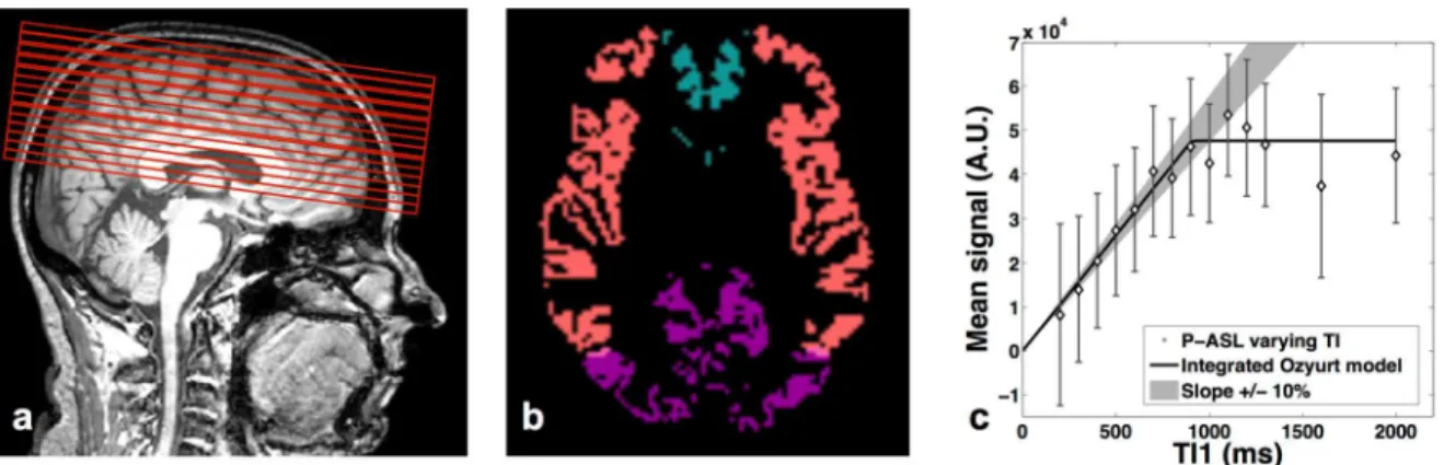
data. The mean difference between control and tag images was calculated to obtain a vascular ASL signal map at each TI. Using the Brain Extraction Tool (bet2) from FSL[15] data from non-brain tissue were eliminated. To automatically select voxels with arterial signal, four large regions approximately corresponding to anterior cerebral artery (ACA), posterior cerebral artery (PCA), and left and right middle cerebral artery (MCA) vascular territories were defined (Figure 1b). The area under the bolus curve (AUC) was computed for each voxel and voxels with at least 20% of the maximal AUC in each territory were selected. The cluster of connected voxels with the highest cumulative AUC in each of the four vascular territories was retained as ROI for the subsequent analysis. We fitted the bolus in each voxel from each ROI with the model of Ozyurt [I] based on a modified version of Hrabe-Lewis model to account for the dispersion of the labeled bolus[11] (Figure 1c):
[I]
where A is an amplitude factor, T1B is the T1 of the arterial blood, 1 is the natural width of the
bolus of tagged spins, 2t is the transit delay between label region and imaging slice and k is the dispersion constant. A four-parameter fit was performed using the Levenberg-Marquardt algorithm[16], adjusting A, 1, 2t and k on a per-voxel basis.
After averaging the model curves from each voxel of the ROIs, we extracted the full width at half-maximum from the average bolus model curve, taking into account the T1 decay
(Figure 1c). We thus obtain a value of the bolus width for each of the four ROIs from each BoTuS dataset.
In order to independently measure the duration of the bolus of labeled blood, we measured and analyzed the ASL signal as a function of TI1, at constant TI2. The ASL signal in a
QUIPSS II sequence is directly proportional to the quantity of labeled blood that leaves the label region prior to TI1. Blood flow can be assumed to be constant during the TI1 period, if
signals are averaged over many repetitions that are not synchronized to cardiac phase[17]. If TI1 is shorter than or equal to the natural duration of the bolus, the ASL signal increases
linearly as a function of TI1. For longer TI1 delays, the ASL signal is independent of TI1, as
all labeled blood has left the label region prior to the saturation pulse. This provides an independent means of measuring the natural duration of the bolus of labeled spins. More standard multi-TI2 ASL signal measurements also provide information about the label width,
but they depend in addition on transit delay, which makes the data less robust to analyze. We acquired a series of 12 PASL datasets varying the TI1 from 200 ms to 1300 ms in 100 ms
increments in a Q2TIPS sequence in randomized order. ASL acquisition parameters were: EPI single shot images, voxel size [4-4-5 mm], 14 slices, 30 pairs of images, tag width=200 mm, label gap=15 mm, TE=24 ms, total acquisition time ~40 min. The minimum TI2 was fixed to 1800 ms. TR and TI2 were mostly independent of TI1, but needed to be
adapted for the shortest and longest TI1-values due to sequence timing constraints. The exact
parameter values used are listed in Table 1. For subjects 11-13 we added measurement points at TI1= 1600 and 2000 ms and used a SENSE factor 2.5 with a TE of 19 ms. The first slice of
the ASL acquisitions is the same as the BoTuS slice (Figure 2a). We acquired a high-resolution T1-weighted structural image to obtain grey and white matter masks using SPM8
(3D GRE TR=8.1 ms, TE=3.8 ms. voxel size [1-1-1.3 mm], 256 mm field of view, 100 contiguous sagittal slices).
All images were realigned, coregistered to the anatomic image and normalized to the MNI ICBM atlas using SPM8 software (SPM, Wellcome Department of Imaging Neuroscience,
http://www.fil.ion.u-cl.ac.uk/spm/). Control and label images were subtracted. Data acquired at a TI2 different from 1800 ms were corrected for T1-decay assuming an arterial blood T1 of
1700 ms[18]. We calculated the average ASL data from the grey matter in MCA, ACA and PCA territories, for each of the 12 acquisitions (Figure 2b). We then plotted the ASL signal as a function of the TI1 and fitted it with the model of Ozyurt integrated over time. To determine
TI1,max, the highest TI1 acceptable for ASL data acquisition according to the multi-TI1 data,
we located the point beyond which the model curve was outside a 10% margin around the initial linear slope (Figure 2c).
Results
BoTuS protocol
The acquisition time of the BoTuS sequence is 78 seconds. Subsequently, about 2 minutes of processing are required to obtain the bolus width in the four vascular territories. From the 104 measurements we made under baseline physiologic conditions, 12 were excluded due to an insufficient quality of fit (R2<0.9). Capnia remained constant throughout all acquisitions under baseline condition.
The differences between the bolus width in the left and right MCA and the ACA for our 13 subjects are not statistically significant (right MCA=(708±121) ms; left MCA=(743±116) ms; ACA=(811±156) ms - mean±std), with a higher inter-individual variability in the ACA territory. However, we measured significantly longer bolus duration in the PCA territory: (1094±211) ms. The mean bolus widths for right and left MCA territories for each subject are spread from 550 ms to 977 ms.
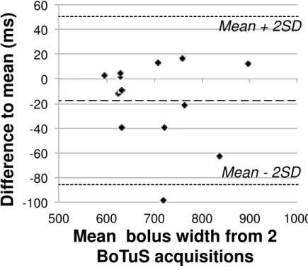
We tested the repeatability of the technique by measuring the bolus shape twice, at an interval of 40 minutes. The repeatability is good as shown in the Bland-Altmann[19] scatter-plot (Fig 3). One subject out of thirteen showed a difference to mean exceeding the 23-interval. The mean difference between the two measurements is significantly different from zero, which implies the presence of an order-effect.
The repeatability coefficient[19] for the measurement of the average bolus width in the right and left MCA territories is 75 ms, that is, the absolute difference between two repeated measurements is expected to be smaller than this value in 95% of the cases. With a mean bolus width of 728 ms in right and left MCA territories for our 26 measurements, this represents a difference of 10% between two measurements on the same subject. The minimum of the bolus widths in left and right MCA territories (instead of their average) showed the same repeatability.
The mean MCA bolus width in 12 subjects (1 subject was excluded due to an insufficient quality of fit (R2<0.9)) was (498±176) ms under hypercapnia (HC) and (747±113) ms under normocapnia (NC) immediately prior to the HC experiment. The analyses of the physiological parameters of our subjects showed no significant difference before and during HC in heart rate (NC=(61±7) min-1 ; HC=(62±7) min-1), arterial oxygen saturation (NC=(98±1)% ; HC=(98±1)%) and respiratory rate (NC=(15±3) min-1 ; HC=(15±3) min-1). The mean end-tidal CO2 increased from (46±6) mmHg during normocapnia to (57±6) mmHg under
hypercapnia. If we assume that the observed reduction in bolus width is inversely proportional to the perfusion change then the mean increase in perfusion due to the CO2 paradigm was
(6±4.3) %/mmHg which is consistent with the literature[20]. The responses to this stimulus were however very heterogeneous between subjects.
Five subjects were excluded due to excessive motion or because the quality of the fit was bad due to a poor signal to noise ratio (R2<0.9). The mean TI1,max on the remaining 8 subjects is
(1020±182) ms for the right and left MCA territories, (1009±250) ms for the ACA territory and (1152±435) ms in the PCA territory. The differences between the three territories are not significant. Also the values in the PCA territories are very heterogeneous and calculated on two subjects only since the others showed a R2 lower than 0.9.
Correlation between BoTuS results and multi-TI1 data
We saw a significant correlation between the bolus width measured in the MCA territory using BoTuS method and the TI1,max determined from multi-TI1 data, with a Pearson
coefficient of 0.65 (p<0.05) (Figure 4a). The bolus width derived from the pre-scan under-estimated the allowable TI1 obtained by the multi-TI1 method, as attested by the scatter plot.
Discussion
The rapid bolus shape pre-scan (acquisition time of 1’18”) allowed determining an optimized TI1 for each subject. The pre-scan acquisition time is dramatically reduced compared to the 40
minutes of acquisitions needed to obtain the bolus width using the 12 PASL multi-TI1 data
points. There are significant differences in the measured bolus widths between vascular territories. Indeed, the PCA are predominantly fed by the basilar arteries, which exhibit slower flow than the ICA predominantly feeding the MCA[21]. This slower velocity generates a longer bolus. The higher inter-individual variability that we observed on the ACA territories is certainly due to the heterogeneities of the ROI in that region. The right and left
MCA territories are the most homogeneous regions since we selected the middle cerebral arteries just above the circle of Willis. The repeatability of the BoTuS technique in this territory is good as shown in the Figure 3.
The estimation of the allowable TI1 from the multi-TI1-data is taken as a reference since it
directly samples the ASL signal of interest. However, it suffers from low SNR. The long acquisition times make the results prone to motion artifacts and prevented us from assessing its repeatability. Almost 40% of the multi-TI1-data had to be discarded. To somewhat
alleviate the problem of SNR, and because the bolus duration is shorter in this territory, we used the large MCA territories (12400 voxels on average) to examine the correlation with the BoTuS method. The results in the ACA and PCA territories are more variable due to the small ROIs, given the position of the imaging volume above the circle of Willis (1950 and 1290 voxels, respectively).
The significant correlation between the BoTuS and the multi-TI1 methods indicates that our
BoTuS sequence has the potential for optimizing PASL acquisitions. However, the BoTuS results are not immediately comparable to the multi-TI1 data, since the TI1,max is a measure of
the integral under the bolus curve. A calibration is therefore necessary to translate the width at half maximum of the roi-average bolus model to a subject-optimized TI1. The limited
multi-TI1 data available in this study leads us to an empirical calibration:
TI1,sequence=1,2*TI1,BoTuS,MCA (Figure 4b).
The bolus widths measured by multi-TI1 PASL in the MCA territory with a 200-mm label
region vary from 717 ms to 1226 ms. With the choice of a fixed TI1 of 700 ms, perfusion
would be quantified accurately for all of our subjects under baseline physiologic conditions. If we determine a per-subject TI1 using the rapid BoTuS pre-scan and our calibration, one
On the other hand, with TI2=1800 ms, the optimized TI1 would lead to an average gain of
18% in ASL signal, with respect to the fixed TI1 of 700 ms.
The ASL literature is relatively sparse in data concerning the optimal choice of TI1 depending
on label width, position, and subject population. From the limited data presented here it is obvious that inter-subject heterogeneity in label duration is large. The method presented has the potential to avoid the need for time-consuming optimizations of this parameter, and to render protocols more robust to variations in slice positioning and subject physiology and morphology.
Bibliography
[1] J. A. Detre, J. S. Leigh, D. S. Williams, et A. P. Koretsky, « Perfusion imaging »,
Magn Reson Med, vol. 23, no. 1, p. 37–45, 1992.
[2] R. B. Buxton, L. R. Frank, E. C. Wong, B. Siewert, S. Warach, et R. R. Edelman, « A general kinetic model for quantitative perfusion imaging with arterial spin labeling. », Magn
Reson Med, vol. 40, no. 3, p. 383–396, 1998.
[3] E. C. Wong, R. B. Buxton, et L. R. Frank, « Quantitative imaging of perfusion using a single subtraction (QUIPSS and QUIPSS II). », Magn Reson Med, vol. 39, no. 5, p. 702–708, 1998.
[4] W. M. Luh, E. C. Wong, P. A. Bandettini, et J. S. Hyde, « QUIPSS II with thin-slice TI1 periodic saturation: a method for improving accuracy of quantitative perfusion imaging using pulsed arterial spin labeling. », Magn Reson Med, vol. 41, no. 6, p. 1246–1254, 1999. [5] R. B. Buxton, « Quantifying CBF with arterial spin labeling. », J Magn Reson
Imaging, vol. 22, no. 6, p. 723–726, 2005.
[6] E. T. Petersen, T. Lim, et X. Golay, « Model-free arterial spin labeling quantification approach for perfusion MRI », Magn Reson Med, vol. 55, no. 2, p. 219–232, 2006.
[7] M. E. Kelly, C. W. Blau, et C. M. Kerskens, « Bolus-tracking arterial spin labelling: theoretical and experimental results », Phys Med Biol, vol. 54, no. 5, p. 1235–1251, 2009. [8] D. S. Bolar, T. Benner, J. B. Mandeville, A. G. Sorensen, et R. D. Hoge, « Accuracy of Pulsed Arterial Spin Labeling in the Brain: Tag Width and Timing Effects », ISMRM
proceeding, 2004.
[9] M. Villien, E. Chipon, I. Troprès, S. Cantin, J.-F. Le Bas, A. Krainik, et J. M. Warnking, « Validation of the per-subject chracterization of bolus width using multi-phase
pulsed Arterial Spin Labeling ». ESMRMB proceeding, 2011.
[10] E. Chipon, A. Krainik, I. Troprès, J.-F. Le Bas, C. Segebarth, et J. M. Warnking, « Per-subject characterization of the bolus shape in pulsed arterial spin labeling », ESMRMB
proceeding, 2008.
[11] O. Ozyurt, A. Dincer, et C. Ozturk, « A modified version of Hrabe-Lewis Model to account dispersion of labeled bolus in Arterial Spin Labeling ». ISMRM proceeding, 2010. [12] J. Hrabe et D. P. Lewis, « Two analytical solutions for a model of pulsed arterial spin labeling with randomized blood arrival times. », J Magn Reson, vol. 167, no. 1, p. 49–55, 2004.
[13] M. A. Chappell, B. J. MacIntosh, M. W. Woolrich, P. Jezzard, et S. J. Payne, « Modelling dispersion in Arterial Spin Labelling with validation from ASL Dynamic Angiography ». ISMRM proceeding, 2011.
[14] N. Ashjazadeh, S. Emami, P. Petramfar, E. Yaghoubi, et M. Karimi, « Intracranial Blood Flow Velocity in Patients with 4-Thalassemia Intermedia Using Transcranial Doppler Sonography: A Case-Control Study », Anemia, vol. 2012, p. 798296, 2012.
[15] S. M. Smith, « Fast robust automated brain extraction », Hum Brain Mapp, vol. 17, no. 3, p. 143–155, 2002.
[16] S. Roweis, « Levenberg-marquardt optimization », Notes, University Of Toronto, 1996.
[17] S. M. Kazan, M. A. Chappell, et S. J. Payne, « Modelling the effects of cardiac pulsations in arterial spin labelling », Phys Med Biol, vol. 55, no. 3, p. 799–816, 2010.
[18] H. Lu, C. Clingman, X. Golay, et P. C. M. van Zijl, « Determining the longitudinal relaxation time (T1) of blood at 3.0 Tesla », Magn Reson Med, vol. 52, no. 3, p. 679–682, 2004.
two methods of clinical measurement », Lancet, vol. 1, no. 8476, p. 307–310, 1986.
[20] A. Battisti-Charbonney, J. Fisher, et J. Duffin, « The cerebrovascular response to carbon dioxide in humans », J. Physiol. (Lond.), vol. 589, no. Pt 12, p. 3039–3048, 2011. [21] N. Bowler, D. Shamley, et R. Davies, « The effect of a simulated manipulation position on internal carotid and vertebral artery blood flow in healthy individuals », Man
Ther, vol. 16, no. 1, p. 87–93, 2011.
[22] E. C. Wong, R. B. Buxton, et L. R. Frank, « Implementation of quantitative perfusion imaging techniques for functional brain mapping using pulsed arterial spin labeling », NMR
Tables and Figures TI1 (ms) 200 300 400 500 600 700 800 900 1000 1100 1200 1300 1600 2000 TI2 (ms) 1800 1800 1800 1800 1800 1800 1800 1800 1800 1900 2100 2100 2300 2700 1TI (ms) 1600 1500 1400 1300 1200 1100 1000 900 800 800 900 800 700 700 TR (ms) 3500 3400 3300 3200 3100 3000 3000 3000 3000 3000 3100 3000 3000 3400
Table 1. Acquisition parameters of multi-TI
1images
(TI
1: Time between label
and QUIPSS saturation, TI
2: time between label and acquisition of the first slice,
5TI=time between saturation and acquisition (TI
1+5TI=TI
2), TR: time between
successive tag and control label pulses)
Figure1: a) Position of the BoTuS acquisition slice just above the circle of
Willis, b) ROIs of connected voxels with strong vascular signal in right and left
middle cerebral arteries, and in the anterior and posterior area, c) Normalized
control/tag difference from the BoTuS sequence showing the bolus shape of the
tagged spins entering our regions of interest for four vascular territories. The
dashed line indicates the cutoff at half the peak amplitude after correction for
T
1-decay, used to determine the duration of the bolus as indicated by the vertical
lines.
Figure 2: a) Position of the multi-TI
1imaging slices. The first slice of the PASL
region of interest is the same as the BoTuS slice, b) Vascular territory map
(pink: middle cerebral arteries, blue: anterior cerebral arteries, purple: posterior
cerebral arteries), c) Average ASL signal in the gray matter of the MCA
territories as a function of TI
1for a single subject. The solid line represents the
fit to the data and the shaded region indicates the limits of the linear regime of
the ASL signal.
Figure 3: Repeatability of the BoTuS results shown in a Bland-Altmann graph
representing the difference to the mean for two separate measurements as a
function of their mean.
-100 -80 -60 -40 -20 0 20 40 60 500 600 700 800 900 1000
D
if
fe
re
n
c
e
t
o
m
e
a
n
(
m
s
)
Mean bolus width from 2
BoTuS acquisitions
Mean + 2SD
Mean - 2SD
R² = 0,42235 500 600 700 800 900 1000 1100 1200 1300 500 700 900 1100 1300 B o T u S , b o lu s w id th ( m s )Multi-TI1, bolus width (ms)
Unity Line BoTuS Linear Correlation R² = 0,42235 500 600 700 800 900 1000 1100 1200 1300 500 700 900 1100 1300 B o T u S , b o lu s w id th ( m s )
Multi-TI1, bolus width (ms)
Unity Line BoTuS 1 BoTuS 2 Linear Correlation