Second Order Fluid Glow Discharge Model Sustained by Different Source Terms
This article has been downloaded from IOPscience. Please scroll down to see the full text article. 2011 Plasma Sci. Technol. 13 583
(http://iopscience.iop.org/1009-0630/13/5/14)
Download details:
IP Address: 66.194.72.152
The article was downloaded on 09/08/2013 at 18:59
Please note that terms and conditions apply.
View the table of contents for this issue, or go to the journal homepage for more Home Search Collections Journals About Contact us My IOPscience
Second Order Fluid Glow Discharge Model Sustained by Different
Source Terms
D. GUENDOUZ1, A. HAMID2, A. HENNAD2
1Institute of Maintenance and Industrial Security, University of Oran, Algeria
2Electrical Engineering Department, Oran University of Sciences and Technology, Algeria
Abstract
Behavior of charged particles in a DC low pressure glow discharge is studied. The electric properties of the glow discharge in argon, maintained by a constant source term with uni-form electron and ion generation, between two plane electrodes or by secondary electron emission at the cathode, are determined. A fluid model is used to solve self-consistently the first three moments of the Boltzmann equation coupled with the Poisson equation. The stationary spatial distribution of the electron and ion densities, the electric potential, the electric field, and the electron energy, in a two-dimensional (2D) configuration, are presented.Keywords: glow discharge, Boltzmann equation, Poisson equation, electron temperature
PACS:
52.30.Ex, 52.65.-y, 52.80.Hc1
Introduction
The field of cold plasma technology has been devel-oped during recent decades to cover a great number of applications whose environmental and economic reper-cussions are extremely important. For this reason, glow discharge has been studied experimentally and theoret-ically[1,2]. Such applications are witnessed in different fields, such as the etching and deposition of thin lay-ers, purity analysis, low pressure gas discharge lamps and plasma display screens. The cold plasmas of glow discharges or corona discharges are characterized by a ratio of electron temperature to gas temperature above 1000. Because of these thermodynamic properties of cold plasmas, this type of discharge is particularly well suited for the surface treatment of heat sensitive mate-rials, such as polymers.
The first attempt to model cathode fall character-istics was made by WARD[3], DAVIES et al.[4] and NEURINGERV[5]using the coupled differential equa-tions for the electron flux and electric field. BAYLE et al.[6] also studied the cathode region of a transi-tory discharge in CO2. In 1986, GRAVES et al. [7] pre-sented a continuum model of DC and RF discharges based on balance equations for charged particles and electron energy densities and Poisson’s equation, as well as for the total electron energy flow and ionization rate. The mathematical models containing the electronega-tive gas composition were made by BOEUF[8]. The model consists of three continuity equations of charged particle species coupled self-consistently with Poisson’s equation, but the electron energy dependence of the re-action rates was not taken into account in the discharge simulation.
Our work aims to introduce a source term includ-ing the electron energy dependence in the continuity
equations of the second order fluid model of the glow discharge. In section 4, a study with a uniform elec-tron and ion generation source is developed. Section 5 presents a study in which a glow discharge is sustained by a secondary electron emission at the cathode.
2
Fluid model
The physical model of glow discharge presented in this work is a second order fluid model, where the charged particle’s transport is described by a macro-scopic quantity. It is based on the resolution of the first three moments of the Boltzmann equation. These three moments are continuity, momentum transfer and energy equations, which are coupled with the Poisson equation by considering the balance approximations of the local field and the average local energy. In this model, the charged particles considered are electrons and positive ions (Ar+).
The transport equations for each charged particle species and the Poisson equation can be described by the equation system as follows,
∂ne
∂t + ∇rΦe= Se(εe), (1)
Φe = −µeneE − ∇(Dene), (2)
∂n+ ∂t + ∇rΦ+= S+(εe), (3) Φ+= µ+n+E − ∇(D+n+), (4) ∂neεe ∂t + 5 3∇rΦε= Sε(εe), (5) Φε= −µeEneεe− ∇(Deneεe), (6) ∆V = −e ε0 (n+− ne), (7)
Plasma Science and Technology, Vol.13, No.5, Oct. 2011
where ne, n+, Φe, εeΦε, E, V , De, D+, µe, µi, e and
ε0are, respectively, electron and ion densities, electron and ion fluxes, electron energy and energy flux, elec-tric field and potential, electron and positive ion diffu-sion coefficients, electron and ion mobilities, elementary charge, vacuum permittivity. S are the source term, which will be defined according to the source used.
3
2D Resolution method
The numerical method adopted in our model is sim-ilar to that described by SCHARFETTER and GUM-MEL[9] in the context of electron transport in semi-conductors. The electron and ion fluxes are discretized using the finite difference method based on the expo-nential flux scheme and Poisson equation using the cen-tered finite differences method. The basic idea of the exponential scheme is to assume that the particle flux is constant between mesh points. The integration time step is kept constant[10].
Eqs. (1), (3), (5) to be resolved have the same gen-eral form,
∂n(x, y, t)
∂t + K∇rΦ(x, y, t) = S(x, y, t), (8)
where n can be an electron or ion density, Φ an electron or ion flux, so the constant K is equal to one (K = 1) and S = Se or S = S+, or n can be an energy density
(neεe), and Φ an energy flux, so K = 5/3 and S = Se. The transport Eq. (8) and Poisson Eq. (7) have a general form and can be developed in 1D and 2D con-figurations. In our 2D work, these equations take the following forms, ∂n(x, y, t) ∂t + K ∂Φ(x, y, t) ∂x + K ∂Φ(x, y, t) ∂y = S(x, y, t), (9) δ2V (x) δx2 + δ2V (x, y) δy2 = − e ε0(ni− ne). (10) Using the finite difference method, these equations be-come nk+1i,j − nk i,j ∆t + K Φk+1 i+1/2,j− Φk+1i−1/2,j ∆x +KΦ k+1 i,j+1/2− Φ k+1 i,j−1/2 ∆y = S k i,j, (11) Vi−1,j+ Vi+1,j ∆x2 + Vi,j+1+ Vi,j+1 ∆y2 −2Vi,j( 1 ∆x2+ 1 ∆y2) = − e ε0(n+i,j− nei,j), (12) where the particle flux or energy flux expression at k+1 instant and at (i + 1/2, j) position is
Φk+1i+1/2,j =[n k+1
i+1,jDki+1,j− nk+1i,j Di,jk exp(T1)]T1
∆x2[1 − exp(T1)] . (13)
Also, at (i − 1/2, j) position and (k + 1) instant, Φk+1
i−1/2,j =
nk+1
i,j Di,jk − nk+1i−1,jDi−1,jk exp(T2)T2
∆x2[1 − exp(T2)] . (14) With T1= −s µk i+1/2,j Dk i+1/2,j (Vk i+1,j− Vi,jk), (15) T2= −s µk i−1/2,j Dk i−1/2,j (Vi,jk − Vi−1,jk ), (16)
s = −1 for electrons and s = +1 for positive ions.
A similar expression can also be obtained for Φk+1i,j+1/2, Φk+1i,j−1/2, T3 and T4. After the substitution of the flux expression in Eq. (11), we obtain the following discretized form, n ¯ ¯ ¯k+1 i−1,j h K DLT2expT2 ∆x2(1 − expT2) i + n ¯ ¯ ¯k+1 i,j h 1 ∆t −K DLT1expT1 ∆x2(1 − expT1)− K D2T2 ∆x2(1 − expT2) −K DTT3exp T3 ∆y2(1 − exp T3)− K DTT4 ∆y2(1 − expT4) i +n ¯ ¯ ¯k+1 i+1,j h k DLT1 ∆x2(1 − expT1) i = n ¯ ¯ ¯k+1 i,j h 1 ∆t i +S ¯ ¯ ¯k i,j− n ¯ ¯ ¯k+1 i,j−1 h K DTT4expT4 ∆y2(1 − expT4) i −n ¯ ¯ ¯k+1 i,j+1 h K DTT3expT3 ∆y2(1 − expT3) i . (17)
Matrices (17) and (12) obtained after discretization are tridiagonal. Hence the transport and Poisson equations can be solved with the Thomas algorithm[11]combined with the iterative relaxation method.
4
Uniform particle source
4.1
Model equation
The present study discusses the properties of a class of electrical discharge with a high current, generated when a spatially uniform source of ionization fills the medium between two parallel planar conductive elec-trodes. The source is considered to be independent of the applied electric field. It is assumed that the elec-trodes are perfect absorbers of electrons or ions without electron and ion emission due to thermionic, photoelec-tric, or other secondary processes. Space-charge effects in these discharges are significant, particularly in the electrode-sheath regions.
WARDIAW and COHEN[12] studied the properties of similar discharges in photo ionization chambers. An-alytic properties were derived for different asymptotic limits in the intensity of the ionization source and the applied electric field. The inclusion of the effects of recombination results in qualitatively different types of solution, which include, for example, a uniform positive column.
Examples of discharges discussed in this first study are (1) γ-ray irradiated discharges[13], where photo ion-ization of the gas is generated by γ-rays, (2) plasmas generated by neutron irradiation[13]where volume ion-ization of the gas is carried out by fission fragments gen-erated by neutron-induced disintegration or a suitable target within the discharge tube, and (3) laser glow dis-charges, where volume ionization is carried out by an energetic electron beam[14], which enters the discharge tube through a thin metal window but does not con-tribute directly to the discharge current.
The equation obtained earlier is with a general ex-pression according to the source term used. In the previous study, the glow discharge is maintained by a steady source with a uniform generation for elec-tron and ion[10,15,16]between two parallel planar elec-trodes. The primary source of electrons is the source function S0, giving the number of electron and positive-ion pairs generated/sec cm3, where S0 is considered to be uniform throughout the inter-electrode region. Also, the electron-ionization and recombination collision pro-cesses are included in our model.
Using the local average energy approximations, the source term in Eqs. (1), (3) and (5) becomes
Se= S0+ KioN neexp(−Ei/KBTe) − γnen+, (18)
S+= S0+ KioN neexp(−Ei/KBTe) − γnen+, (19)
Sε= −S0εe− eΦE − neKioN Hiexp(−Ei/KBTe)
+Eiγnen+, (20)
where S0is the net source term of electron and ion pairs generated[13,15]and is equal to 3.6×10²² m−3· s−1; Kio,
Ei, Hi represent the ionization rate factor, ionization activation energy and the energy loss in ionizing colli-sion, respectively; N is the gas density and KB is the Boltzmann constant; γ is the recombination coefficient of ions in argon and is equal to 8.81×10⁻⁷ cm3· s−1 in our case[15].
Eqs. (18) ∼ (20) combined with Eqs. (1), (3) and (5) are discretized according to Eq. (17), with an integra-tion time step of 10−9 s.
4.2
Transport parameters
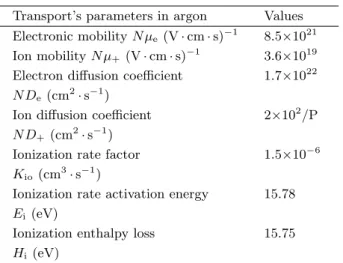
The discharge results have been compared with those of the LOWKE and DAVIES model[15]; we therefore apply the same simulation conditions. The pressure P is set to 240 Torr and the gas temperature is as-sumed to be uniform and equal to 293 K. We use a constant transverse and longitudinal diffusion, i.e.,
DL = DT = D. Table 1 lists the transport parame-ters[17] used in the 2D code.
Table 1. Transport parameters of electrons and ions in argon for constant source term
Transport’s parameters in argon Values Electronic mobility N µe (V · cm · s)−1 8.5×10²¹
Ion mobility N µ+ (V · cm · s)−1 3.6×10¹⁹
Electron diffusion coefficient 1.7×10²²
N De (cm2· s−1)
Ion diffusion coefficient 2×10²/P
N D+ (cm2· s−1)
Ionization rate factor 1.5×10⁻⁶ Kio(cm3· s−1)
Ionization rate activation energy 15.78
Ei(eV)
Ionization enthalpy loss 15.75
Hi(eV)
4.3
Boundary and initial conditions
The inter-electrode distance and electrode width are set to 0.3 cm. In this model, it is assumed that on the dielectric surfaces, both electron and ion densities are equal to zero, while on the electrodes’ surface the elec-tron density is equal to zero and the ion density satisfies the Neumann condition,
∂n+ .
∂x = 0. (21)
The potential applied is void at the cathode surface (x = 0), and fixed to 100 V at the anode surface (x = L), while on the dielectric surfaces it is set in accordance with the following equation[18],
e ε0 t Z 0 [Φ+(t) − Φe(t)]ndt = −∇nV (t). (22) The electron temperature is set to be 0.5 eV at the cathode surface and on other surfaces satisfies the rela-tion
5 2∇Te−
e
kB∇V = 0. (23) The initial distribution for the electron and ion densi-ties takes a Gaussian form[17]written, in (cm−3), by
ne= n+= h 107+ 109(1 − x L) 2(x L) 2+ (1 − y L) 2(y L) 2i. (24) The initial distribution of the electron temperature is assumed to be a constant of 1 eV.
5
Secondary electron emission at
the cathode
5.1
Model equation
In this section, the glow discharge with a low cur-rent is considered to be maintained by electron emis-sion caused by ionic ‘shelling’ at the cathode [19∼21].
Plasma Science and Technology, Vol.13, No.5, Oct. 2011
A numerical code elaborated for the second order fluid model is applied, in which only ionization collision is considered. The source term in Eqs. (1), (3) and (4) becomes
Se= KioN neexp(−Ei/KBTe), (25)
S+= KioN neexp(−Ei/KBTe), (26)
Sε= −eΦeEn− eKiN Hiexp(−E/KBTe). (27)
5.2
Basic data
Table 2 lists all of the basic data and transport pa-rameters[19,20] used in the 2D code.
Table 2. Basic data for argon with secondary electron emission at the cathode effect
Transport’s parameters in argon Values Secondary electron emission coefficient γ 0.046 Ion mobility µi cm2 (V · s)−1 2×10³
Electron mobility µecm2(V · s)−1 2×10⁵
Ion diffusion coefficient Di (cm2· s−1) 102
Electron diffusion coefficient De (cm2· s−1) 106
Ionization rate factor Kio(cm3· s−1) 2.5×10⁻⁶
Ionization rate activation energy Ei (eV) 24
The gas density is set to be 2.83×1016 cm−3 with a gas temperature of 323 K. The electron temperature and energy are linked as follows,
εe= (3/2)KBTe. (28)
The transport coefficient components are asummed to be constant (DL= DT). The results of discharge were compared with those of LIN and ADOMAITIS[19], ex-plaining why we use the same simulation conditions.
5.3
Boundary and initial conditions
In this discharge case, the same conditions were used for the initial and boundary distributions of ion and electron densities and temperatures, on the dielec-tric walls and at the electrode surfaces. The poten-tial applied is set to −77.4 V at the cathode (xmax =
L = 3.525 cm)[19,20] and to zero at the anode (x = 0). The effect of the secondary electron emission coefficient
γ at the cathode appears through the following
condi-tion,
Φe(x, y, t) = −γΦ+(x, y, t). (29)
6
Results and discussion
6.1
Constant source term
In Figs. 1∼6 the stationary 2D spatial distributions of the electric potential and field, electron and ion den-sities and energy of electrons as functions of the inter-electrode distance (x), and inter-electrode width (y), in glow discharge maintained by a constant source with uniform electron and ion generation, are shown, respectively.
Fig.1 Spatial distribution of electric potential
Fig.2 Spatial distribution of longitudinal electric field
Fig.3 Spatial distribution of transversal electric field
The 2D results show the influence of a transverse field. The curves in 2D show clearly three distinct ar-eas, namely the cathode sheath, the positive column and the anodic area. It is a normal discharge regime. In Fig. 1 a significant fall of potential in the cathode region is shown. In the area of the positive column where plasma is formed, the potential is almost con-stant, and roughly equal to the potential applied to the anode. Therefore, in Fig. 2, the variation in longitu-dinal field is linear in the cathode region and equal to zero in the positive column. The direction of the elec-tric field near both electrodes opposes the diffusion of
electrons from the central ionized region to the elec-trodes. The transverse field in Fig. 3 lies within the sense of natural displacement of the charged particles. It is worth to note that this field component is symmet-rical in the middle of the electrode in comparison with the direction of longitudinal shift of the charged parti-cles. It changes its sign on either side of this direction. Hence the transverse electric field drags towards the center of the discharge of the charged particles, which tend to deviate from their axis of motion through ion and electron diffusion.
In Figs. 4 and 5, the first area is also characterized by a negligible electronic density compared with the ion density. The density gradient in this area is due to the fact that the electrons move much faster than the ions in the presence of a potential gradient, which involves an electron depopulation in the area. The pos-itive column area is characterized by a constant and nearly equal electron and ion densities. Consequently, the net space charge is negligible, and the potential is constant. In the anode region, the ion density is rel-atively significant compared with the electron density because of the constant source term.
Fig.4 Spatial distribution of electron density
Fig.5 Spatial distribution of ion density
In Fig. 6, the electron temperature exhibits a max-imum near the electrodes where a high electric field is dominant. The electron temperature increases with the increase in both the longitudinal and the transverse
electric field as seen in the two 2D curves. This ac-quired energy accelerates electrons toward the positive column where they collide with neutrals which causes ionizations and cooling of electrons. In the positive col-umn, where a nearly linear variation in electron temper-ature occurs, electrons continue their displacement to-wards the anode region, where the drop in temperature is sharp due to electron displacement in the opposite direction.
Fig.6 Spatial distribution of electron energy
6.2
Secondary electron emission at the
cathode
In Figs. 7∼12 the steady 2D spatial distribution of the electric potential and field, the ion and electron densities, and the electron temperature in step with the normalized inter-electrode distance (x/L), and elec-trode width (y/L) are shown, respectively. The pres-ence of two different regions, namely the anode region and the cathode-sheath region, is shown clearly. It is a subnormal discharge regime.
A potential fall in the region of the cathodic sheath can be seen in Fig. 7. This is one of the typical charac-teristics for Townsend discharge. In the anode region, the potential varies slightly. In the cathode sheath in Fig. 8 the presence of an intense longitudinal electric field can be seen. This behavior is normal because of the value of the net space charge density, which is not zero in the anode region, shown in Figs. 10 and 11, and the electrons are the major current carrier near the grounded electrode while the ions are the one near the powered electrode. The electron temperature profile in Fig. 12 also gives the electron energy distribution. Elec-trons quickly gain energy from the electric field and are accelerated inwards, so the temperature increases dra-matically near the powered electrode. The curve then quickly dips down due to strong electron cooling by ion-izations, which are highly endothermic. The bulk phase temperature is rather flat and becomes flatter with the increase in voltage drop. The small drop near the an-ode is due to the electrons moving against the electric field. In Fig. 9, the transverse field also changes signs on either side of this direction. The transverse electric
Plasma Science and Technology, Vol.13, No.5, Oct. 2011
field orientates the charged particles towards the center of the discharge.
Fig.7 Spatial distribution of electric potential
Fig.8 Spatial distribution of longitudinal electric field
Fig.9 Spatial distribution of transversal electric field
7
Validity test of the model
7.1
Constant source term
To validate and test our numerical mode of resolu-tion, a study of this discharge type in argon, under the same conditions as those of LOWKE and DAVIES[15] was carried out.
Fig.10 Spatial distribution of electron density
Fig.11 Spatial distribution of ion density
Fig.12 Spatial distribution of electron temperature
In Fig. 13 it is noted that the steady-state spatial distributions of the potential, electric field, ion and elec-tron densities, on the symmetry axes in 2D, are in con-formity with the results of the first order model in 1D given by LOWKE and DAVIES [15]. Their numerical results were validated by experimental results[13].
The first order model in 2D and the second order model in 1D[16,21] are also studied, and the results are in agreement with those of LOWKE and DAVIES.
In Fig. 14, the electron energy curve in 1D devel-oped[21] and the 2D results of the symmetric axes, in the middle of the electrodes, take a similar form, with the magnitude difference due to the presence of two
electric field components in 2D and to the boundary conditions.
Fig.13 Spatial distribution of electron and ion densities in LOWKE’s 1D code and our 2D code of symmetric axes
Fig.14 Spatial distribution of electron energy in 1D code and 2D code of symmetric axes
7.2
Secondary electron emission at the
cathode
To validate and test our numerical model, a study of this discharge in the same conditions as those of LIN and ADOMAITIS[19] and BOUCHIKHI[21] was carried out. It was noted that the steady-state spa-tial distributions of the ion and electron densities in Fig. 15 and the electron temperature in Fig. 16, on the symmetric axis in 2D case, are in conformity with the results obtained by LIN and ADOMAITIS, who used a pseudo-spectral method to discretize the partial differ-ential equation and their boundary conditions.
Fig.15 Spatial distribution of electron and ion density in LIN’s 1D code and our 2D code of symmetric axes
Fig.16 Spatial distribution of electron temperature in LIN’s 1D code and our 2D code of symmetric axes
8
Concluding remarks
A 2D numerical code using the second order fluid equations and two types of source for a low pressure glow discharge is applied. The glow discharge may be maintained by a constant source of electron and ion gen-eration or by secondary electron emission at the cath-ode.
The resultant electric properties of glow discharge obtained for each source type were validated by using a comparative study with those reported in the liter-ature. Calculated results corroborate with previously published simulations. The distribution of electronic temperature in 1D and 2D configurations is also calcu-lated, where the curve in the 2D code of the symmetric axis is in agreement with that obtained with the 1D code.
The studies of DC discharges presented demonstrate the effect of the parameters applied, where two regimes of glow discharge are obtained, namely normal and sub-normal glow discharge. Also, the general form of the source term allows us to consider the recombination, ionization and excitation processes.
We conclude from this study that our numerical code, elaborated for the second order fluid model in 1D and 2D geometry can be applied to conventional glow discharges maintained by different sources in different glow discharge regimes.
To apply the complete approach of local average en-ergy to the second order fluid model, further work is in progress for the electron energy dependence of the electron diffusivity, and recombination coefficient in one and two dimensions. A normal discharge regime is ob-tained for glow discharge susob-tained by secondary elec-tron emission at the cathode.
References
1 Kline L E. 1990, Non Equilibrium Effects in Ion and Electron Transport. Eds. Gallagher J W, Hudson D F, Kunhardt E E, Van Brunt R J. Plenum Press, New York. p.121
Plasma Science and Technology, Vol.13, No.5, Oct. 2011
3 Ward A L. 1962, J. Appl. Phys., 33: 2789
4 Davies A J, Evans J G. 1980, J. Phy. D, 13: 21
5 Neuringer J L. 1978, J. Appl. Phys., 49: 590
6 Bayle P, Vacquie J, Bayle M. 1986, Phys. Rev. A, 34: 360
7 Graves D B, Jensen K F. 1986, IEEE Trans. Plasma Sci., 14: 78
8 Boeuf J P. 1987, Phys. Rev. A, 36: 2782
9 Scharfetter D L, Gummel H K. 1969, IEEE Trans. Electron. Devices, 16: 64
10 Hamid A, Bouchikhi A, Hennad A. 2003, Model of glow discharge in Argon. VIII Plasma Congress of Physics French Society SFP. http://www-fusion mag-netique.cea.fr/sfp 2003/Livre−resume−sfp 2003−
zou.pdf
11 Nougier J P. 1985, Methods of numerical calculation. 2e Masson Edition, Paris
12 Wardiaw A B, Cohen I M. 1973, Phys. Fluids, 16: 637
13 Leffert C B, Rees D B, Jamerson F E. 1966, J. Appl. Phys., 37: 133; also, Boag J W. in Radiation Dosime-try, edited by Attix F H and Roesch W C. (Academic, New York, 1966), Vol. II, Chap. 9, p.1.
14 Fenstermacher C A, Nutter M J, Leland W T, et al. 1972, Appl. Phys. Lett., 20: 56; also, Dreyfus R W, Hodgson R T. 1972, Appl. Phys. Lett., 20: 195
15 Lowke J, Davies K. 1977, J. Appl. Phys., 48: 4991
16 Hamid A. 2005, Mono and bidimensionnal numer-ical model of glow discharge in low pressure DC regime. [Ph.D thesis] Sciences and Technology Mo-hamed Boudiaf University, Oran, Algeria
17 Park S, Economou D J. 1990, J. Appl. Phys., 68: 3904
18 Fiala A. 1995, Two-dimension numerical modelisa-tion of low pressure glow discharge. [Ph.D thesis] Paul Sabatier University, Toulouse, France, no2059
19 Lin Yi-hung, Adomaitis R A. 1998, Physics Letters, A, 243: 142
20 Meyyappan M, Kreskovsky J P L. 1990, J. Appl. Phys., 68: 1504
21 Bouchikhi A, Hamid A. 2010, Plasma Sci. Technol., 12: 59
22 Guendouz D, Hamid A. 2009, IREPHY, 3: 268
(Manuscript received 21 January 2011) (Manuscript accepted 18 April 2011)
E-mail address of D. GUENDOUZ: [email protected]
![Table 2 lists all of the basic data and transport pa- pa-rameters [19,20] used in the 2D code.](https://thumb-eu.123doks.com/thumbv2/123doknet/15047690.693640/5.892.509.768.94.299/table-lists-basic-data-transport-rameters-used-code.webp)
