Different regimes of first order fluid model of glow discharge

Different regimes of first order

fluid model of glow discharge

1

_{Djillalia. Guendouz}

2

_{Azzeddine. Hamid}

Electrotechnic Department,

Sciences and Technology Oran University (USTO) 1_{[email protected]}

2 _{[email protected]}

3

_{Sergey. Pancheshnyi}

Laboratory of Plasma and conversion of energy. Paul Sabatier University,

Toulouse, France

[email protected] Abstract---The objective of this article is to study the kinetics

of charged particles in a glow discharge low pressure in DC mode, sustained by electrons and ions uniform production source. We deduced for the stationary state, the electrics characteristics distributions of the charged particles in a two-dimensional 2D plan-plan configuration. The numerical model presented in this work is based on the first two moment resolution of Boltzmann’s equation.

The characteristics of the glow discharge in argon (densities, field, and potential) according to source term value are presented in this paper. Different types of glow discharge (abnormal, normal, subnormal regime) can be observed that depends of technology application.

Keywords- glow discharge, equation of Boltzmann, constant source term, density of the charged particles, Poisson’s equation.

I. INTRODUCTION

Plasmas of the cold discharges, that are luminescent or crowns, are characterized by a difference between the temperature of the electrons and that of gas, the relationship can be equal to 1000 and more. This absence of balance between the two temperatures makes it possible to obtain plasma in which the temperature of the gaseous medium can be close to the ambient temperature whereas electrons can acquire sufficient high energies to make with the molecules and/or the atoms of gas, inelastic collisions of ionization, attachment or excitation. These thermodynamic properties of these cold plasmas return this type of discharges particularly well adapted in optics, optoelectronics and micro-electronics for the area treatment of metallic material surface dressing sensitive to heat such as polymers, organometallic deposits, multi-layer, engraving of reasons micro and nanometric.

The field of the engineering of cold plasmas developed during the last decades cover a great number of applications [1][2][3][4] whose economic repercussions are extremely significant.

Our work consists in simulating, for the stationary state, the distributions of the electric field and the density of the particles in charge of self-coherent way in two-dimensional geometrical configuration. This configuration, contrary to the one-dimensional model [5][6] enables us to take into account all the transverse parameters. This, places us in a more realistic situation which describes the electric behaviour of the discharges. We can deduce from these distributions the current of the discharge and the power dissipated in the engine with plasma. This model thus makes it possible to reach a better comprehension and optimization of the technological processes based on the

use of cold plasmas in industry. The gas used for this simulation is monatomic electropositive gas argon. The digital model presented in this work is based on the first two moment’s resolution of Boltzmann’s equation.

In section II we present equations of first order fluid model, in section III and IV we develop the resolution method of transport equations of fluid model.

The characteristics of the glow discharge in argon (densities, field and potential) in two dimensional Cartesian geometrical configurations are presented in section VI.

II.DESCRIPTION OF THE FIRST ORDER FLUID MODEL

In our work, the model presented is subject to the following assumptions: (1) the discharge is weakly ionised so that the discharge physics problem can be decoupled from the transport of neutral gas. In addition electron-electron collision is negligible. This assumption is usually satisfied for discharge used in electronics-materials processing since the charged particle-to-neutrals ratio is usually below 10-4_{. (2) Particle loss through gas} convective motion is negligible, (3) electrons emission at the cathode is negligible, ionization and recombination collision process are considered in our model.

The governing equations used in this study are the first two moments of the Boltzmann transport equations. These two moments are the equations of continuity and transfer of the momentum which are coupled with the Poisson's equation by using the approximation of the local field. In this approximation, we suppose that there is a compensation of the charged particles energies gained by the electric field and lost by collisions of. This assumption of local balance can be used as a relation of closing for a system of equations of Boltzmann’s equations, which describes the kinetics of the particles charged. A simple model comprising only electrons and positive ions Ar+ (case of argon) in two-dimensional geometry, can then be consisted by the system of equations according to the following:

+∇Φ = + − ₊ ∂ ∂ n n n S t n e e e e e ' _{αμ E γ . (1)} Φe =−neμeE−De∇ne. (2) + _{+∇Φ+ = + − +} ∂ ∂ n n n S t n e e eαμ E γ ' _{. (3)} 978-1-4244-6255-1/11/$26.00 ©2011 IEEE

Φ₊ =n₊μ₊E−D₊∇n₊. (4) ( ) 0 e n n e V =− − Δ _ε + . (5)

In the above equations we use the following notation: • ne and n+ are electron and positive ion density. • De and D+ are electron and ion diffusion

coefficient.

• μe , μ+ are electron and ion mobility.

• Φ ,e Φ are electron and ion flux components in ₊

the x and y directions.

• E and V are the electric potential and field, • e is elementary charge, ε0 vacuum permittivity.

• S’ represents the constant source term of the electrons and ions uniform production to sustain the discharge [7].

• Parameter

α

is Townsend’s first ionisation coefficient

•

γ

is the recombination coefficient of the ions in argon.

III.DISCRETIZATION OF THE TRANSPORT EQUATIONS

The transport equations (1), (3) and Poisson’s equation (5) to be solved have following form in 2D:

S y t y x x t y x t t y x n = ∂ Φ ∂ + ∂ Φ ∂ + ∂ ∂ ( , , ) ( , , ) ( , , ) _{. (6)} (n n ) ε e δy V(x,y) δ δx V(x) δ e i− − = + 0 2 2 2 2 . (7) The numerical schema adopted in our model is similar to that is described particle transport in semi conductors by Scharfetter and Gummel [8]. The basic idea of the exponential scheme of Scharfetter and Gummel is to assume that the particle flux is constant between mesh points. The step of integration in time is set constant.

The equations (6) and (7) are approximated with the following using finite difference method:

t n n k j i k j i Δ − + , 1 , + x k j i k j i Δ Φ − Φ + − + + 1 , 2 / 1 1 , 2 / 1 + k j i k j i k j i S y , 1 2 / 1 , 1 2 / 1 , = Δ Φ − Φ + − + + _. (8) ) n (n ε e ) Δy Δx ( V Δy V V Δx V V i,j e i,j i,j i,j i,j ,j i ,j i − − = + − + + + + + + + − 0 2 2 2 1 1 2 1 1 ₂ 1 1 With: (9) k j i k j i k j i k j i k j i k j i k j i k j i k j i w D w x D D w x Y Y , 2 / 1 1 , 2 / 1 , 2 / 1 1 , 2 / 1 1 , 2 / 1 , 2 / 1 1 , 1 , 1 1 , 2 / 1 / )) / exp( 1 ( ) / exp( + + + + + + + + + + + + + + Δ − Δ − = Φ .(10) Where: k j 1/2, i j 1/2, i , 2 / 1 +

E

+ +

=

μ

k j i

w

. (11) k j i k j i k j i

n

D

Y

1 _1, , 1 1 , 1 + + + + +

=

. (12) k j i k j i k j i

n

D

Y

1 _, , 1 , + +

₌

_{. (13)} , , ,Φ

μ

n w, D, S are, respectively the particle number

density, flux, mobility, drift velocity, diffusion coefficient and source term.

So the discretized form of longitudinal and transverse electric field is:

x

V

V

k j i k j i

Δ

−

−

=

+ + , , 1 k j 1/2, i

E

. (14)

y

V

V

k j i k j i

Δ

−

−

=

+ + , 1 , k 1/2 j i,

E

. (15) )) exp( 1 ( )) exp( ( 1 2 1 1 , 1 , , 1 1 , 1 1 , 2 / 1 T x T T D n D n k j i k j i k j i k j i k j i − Δ − = Φ + + + + + + . (16)

Where T is defined by: 1

( 1, , ) , 2 / 1 , 2 / 1 1 k j i k j i k j i k j i V V D s T =− + − + + μ . (17) k j i V, is the potential at k

t time on mesh (i, j), s = -1 for electrons and s = +1 for positive ions.

Similar expression can be obtained for Φk_i−+₁1_/2,j for, k 1 2 / 1 j , i++ Φ , k 1 2 / 1 j , i+− Φ .and T2, T3, T4.

After substitution of flux expression in equation (8) the following scheme is obtained:

(

)

⎥⎦+ ⎤ ⎢ ⎣ ⎡ − Δ + − 2 2 2 2 1 , 1 exp 1 exp T T x T D nk L j i 1 , + k j i n

[

(

−

)

−Δ

(

−

)

− Δ − Δ 2 2 2 2 1 2 1 exp 1 exp 1 exp 1 T x T D T T x T D t L L

]

) exp 1 ( ) exp 1 ( exp 4 2 4 3 3 2 3 T y T D T T y T DT T − Δ − − Δ +

(

)

⎥⎦ + ⎤ ⎢ ⎣ ⎡ − Δ + ⎥ ⎦ ⎤ ⎢ ⎣ ⎡ − Δ + − + + 4 4 2 4 1 1 , 1 2 1 1 , 1 exp 1 exp ) exp 1 ( y T T T D n T x T D n k T j i L k j i ⎥ ⎦ ⎤ ⎢ ⎣ ⎡ − Δ + + _{(1 exp )} 3 2 3 1 1 , T y T D nk T j i = k j i k j i S t n , , + Δ . (18)

D_{L and DT are the diffusion coefficient components in x}

and y directions. On the interval [ Xi, Xi+1] and [Yi, Y_i+1 ] we suppose that the diffusion coefficients and mobility’s are constant.

IV.ITERATION RESOLUTION PROCEDURE

Equations (9) and (18) obtained after discretization constitute tridiagonal matrix. Of this fact transport and

Poisson’s equations are solved alternatively with Thomas’s algorithm combined with the iterative relaxation method [9]. Solutions n are obtained for

V n

ne, +,Φe,Φ+, and E, as a function of axial position. The only input experimental parameters are the electrode separation d, the applied voltage V and the source

function S. The material functionsα,γ,w,D, and μ must be specified for the particular gas density considered. The following iteration procedure is used:

• Initial arbitrary profiles are assumed for n as e n a + function of x and y.

• V and E are calculated from n and e n using + equations (9), (14 ) and (15).

• ∂ne ∂tand ∂n+ ∂tare evaluated from the right-hand

sides of equations (1) and (3), and new values of ne and n+ are calculated.

• The new system obtained is written: Therefore for each value of the index j, there will be the tridiagonal matrix which will be solved by the algorithm of Thomas [9]. The values 1

, 1 + k j n and k+1 nx

n are known to the boundary conditions

• The procedure is then repeated, and new profiles for ,n₊

ne and V are generated until convergence is

obtained.

• Because profiles of ne and n+ change very slowly with successive iterations, a test is necessary to ascertain whether profiles have converged. The test adopted is whether derived values of the total current density c, wherec=Φe−Φ₊, are constant for all grid points. This is necessary condition of equations (1) and (3) in the steady state, since when∂ne ∂t=∂n+ ∂t=0 , ∂Φe ∂x=∂Φ+ ∂x, . 0 x ) (Φ_e−Φ ∂ =

∂ ₊ In the present calculations,

convergence is assumed when c is constant to within 5%.

With an aim of accelerating even more convergence of the system of equations, we use a factor of relaxation ω [9]_{.ranging between the value 1 and 2 which is in fact a} coefficient by which we multiply the presumably known densities 1 1 , + − k j i n and 1 1 , + + k j i

n . In general, the value of this factor ω is not known. Ain the case, some tests are necessary to determine it.

V. BOUNDARY CONDITIONS AND TRANSPORT

PARAMETERS

a) In our model, two boundary conditions are required for densities n and e n and electric potential V: i

• At the cathode (x = 0), the anode (x = d), and at the electrodes (y = 0, y = d) the electron and ion densities are taken as zero.

• Generally, we make V = 0 at the cathode V = Va at the anode. Va is the applied voltage. On the electrodes electrical potential satisfy NEUMAN condition:

∂V_∂x=0_{. (19)} b) The temperature and the pressure of the system are

constant [7] and equal respectively to 293°K and 240 Torr.

c) The ionic and electronic diffusion coefficients, as well as their mobility are required as function ofE/N. In the present calculations, we have negligible their data values variation in the interval where the variation of the electric field is weak. So the coefficients ND and Nμ are taken as constant, where N is gas density, and consequently we chooseDL =DT.

d) The ionisation coefficient is given by the following relation, in the case of argon [7]:

_α/N₌4.910−17exp(₋1.4810−15N/E) (cm2)_{. (20)} e) The recombination coefficient is set constant [7], it is

equal to 8.81 10 -7 (cm3_s-1_).

The transport parameters used in our code for argon [10] are consigned in the table below:

TABLE I: TRANSPORT PARAMETERS OF ELECTRONS AND IONS IN

ARGON

Transport’s parameters in argon Values Electronic mobility Nμ_e (V cm s)-1

Ion mobility Nμ₊ (V cm s)-1

Electron diffusion coefficient NDe (cm-1s-1)

Ionic diffusion coefficient D+ (cm 2s-1).

8.5 ×1021 3.6 × 1019 1.7 × 1022

2×102_/P .

VI. RESULTS AND DISCUSSION

Numerical results are presented for three different types of discharges. These discharges correspond to the experimental conditions of Leffert and Al. [11] for argon at 240 Torr, for uniform source functions of 8×1011cm-3 sec-1_{, produced by photo ionization due to γ rays , and} 3.6×1016 _cm-3 _sec-1_{, produced by ionization due to fission} fragments.

The study results presented in this paper concern a two-dimensional Cartesian geometry; the discharge is assumed to be uniform and infinite in the z direction perpendicular to the (x, y) plane. Only steady-state glow discharge will be considered in this following. Argon has been used as a working gas. The inter-electrodes distance and their width are set to 0.3 cm. The two-dimensional distributions of the potential, the electric field, the density of the charged particles and the term source S in a stationary state are presented to illustrate the behaviour of the glow discharge in the subnormal, normal and abnormal regime.

A. Subnormal glow discharge

The subnormal regime of glow discharge have been obtained with our 2D numerical code with uniform source term S’= 8.0×1013 _(cm-3_s-1_{) and the applied voltage to} 105 V.

For solutions appropriate to a γ rays ionization chamber, the sheath thickness is greater than the inter electrodes spacing, and there is no plasma region. Since the drift velocity is of the order 100 times the ion drift velocity.

The results in figures (1) to (6) show the absence of the positive column in space inter-electrodes. There is imbalance between the maxima of ionic and electronic density; the electron density is lower than the positive-ion density.

The surface occupied by the ions and the electrons is different. The electrons are in the vicinity of the anode with a symmetrical space distribution around the axis of the discharge. On the other hand, the distribution of the ionic density is quasi isotropic in space inter-electrodes except near of anode.

0.0 5.0e+7 1.0e+8 1.5e+8 2.0e+8 0.05 0.10 0.15 0.20 0.25 0.05 0.10 0.15 0.20 0.25 E le ct ro n de ns ity ( cm -3) X (c m) Y (cm)

Figure 1. Spatial distribution of electron density in subnormal regime. 0.0 5.0e+8 1.0e+9 1.5e+9 2.0e+9 2.5e+9 3.0e+9 0.05 0.10 0.15 0.20 0.25 0.05 0.10 0.15 0.20 0.25 Io n de ns ity ( cm -3) X (c m) Y (cm)

Figure 2. Spatial distribution of ion density in subnormal regime

0 20 40 60 80 100 120 0.05 0.10 0.15 0.20 0.25 0.05 0.10 0.15 0.20 0.25 E le ct riq u e P o te n tia l (v o lt) X (c m) Y (cm)

Figure 3. Spatial distribution of electric potential regime.

-7 -6 -5 -4 -3 -2 -1 0 0.05 0.10 0.15 0.20 0.25 0.05 0.10 0.15 0.20 0.25 L on gi tu di na l e le ctr ic fi el d ( kv c m -1) X (c m) Y (cm)

Figure 4. Spatial distribution of longitudinal electric field.

-8 -6 -4 -2 0 2 4 6 8 0.05 0.10 0.15 0.20 0.25 0.05 0.10 0.15 0.20 0.25 T ran sv er se e lec tr ic f iel d (k v cm -1) X (c m) Y (cm)

Figure 5. Spatial distribution of transverse electric field

7.0e+13 8.0e+13 9.0e+13 1.0e+14 1.1e+14 1.2e+14 1.3e+14 1.4e+14 0.05 0.10 0.15 0.20 0.25 0.05 0.10 0.15 0.20 0.25 N et s ou rc e T er m e ( cm -3 s -1) X (c m) Y (cm)

This situation indicates to us that the ionic and electronic density did not modify the uniform geometrical field yet and we note (fig 1) that there is a beginning of formation of a pseudo positive column which can extend gradually towards cathode with the increase of the source term.

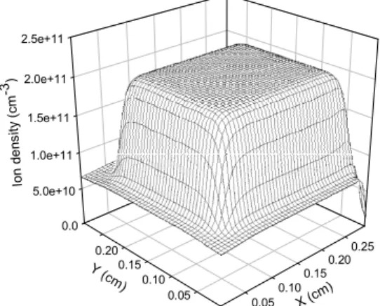
B. Normal glow discharge

The normal regime of the glow discharge was obtained by our 2D numerical model by modifying the source term and the applied voltage.

The uniform source term is set: S’=3.6×1016(cm-3s-1) with an applied voltage of 100 V.

Figures (7) and (8) represent the electronics and ionic densities space distribution in a stationary state of the discharge. They clearly show the presence of three distinct areas: the cathode sheath, the positive column and the anodic area.

0.0 5.0e+10 1.0e+11 1.5e+11 2.0e+11 2.5e+11 0.05 0.10 0.150.20 0.25 0.05 0.10 0.15 0.20 0.25 E le ct ro n D en si ty ( cm -3) X (cm) Y (c_m)

Figure 7. Spatial distribution of electron density in normal regime

0.0 5.0e+10 1.0e+11 1.5e+11 2.0e+11 2.5e+11 0.05 0.100.15 0.200.25 0.05 0.10 0.15 0.20 I on d e ns ity ( cm -3) X (cm) Y (c_m)

Figure 8. Spatial distribution of ion density in normal regime

The first area is characterized by a negligible electronic density compared to the density of the ions. This gradient of density in this area is due to the fact that the electrons move much more quickly than the ions in the presence of a gradient of potential what involves the depopulation of this area by the electrons. The area of the positive column, where plasma is formed, is characterized by electronics and ionic densities which are constant and

quasi equal. Consequently, the space charge is negligible. The maximum of the density for the species charged in this area is 2×1011 _(cm-3_s-1_{). In the anodic} region, the ionic density is relatively significant compared to the electronic density because of the constant source term.

On figures (9), (10) and (11) we respectively represented spatial distribution of the electric potential, and the longitudinal and transverse field in a stationary state. 0 20 40 60 80 100 120 0.05 0.10 0.150.20 0.25 0.05 0.10 0.15 0.20 E le ct ric P ot en tia l ( vo lt ) X (cm) Y (c_m)

Figure 9. Spatial distribution of electric potential in normal regime

-6 -5 -4 -3 -2 -1 0 1 0.05 0.10 0.15 0.20 0.25 0.05 0.10 0.15 0.20 0.25 Lo ng itu di na l e le ct ri c fie ld ( kv c m -1) X (c m) Y(cm)

Figure 10. Spatial distribution of longitudinal electric field.

-8 -6 -4 -2 0 2 4 6 8 0.05 0.10 0.15 0.20 0.25 0.05 0.10 0.15 0.20 0.25 T ra nsve rse e le ct ri c fie ld (k v cm -1) X (c m) Y(cm)

Figure (12) represents the spatial distribution of the net source term S of production of electron-ion pairs in a stationary state. It is significant in the cathode and anode region because of the electric field reigning in these two areas of the discharge.

In the positive column, the net source term S decreases because of two collisionnel process: by ionic recombination and the quasi-total absence of ionization due to the very weak variations of the electric field in this area. 0 1e+16 2e+16 3e+16 4e+16 5e+16 6e+16 0.05 0.10 0.15 0.20 0.25 0.05 0.10 0.15 0.20 0.25 N et s ou rc e T er m e ( cm -3 s-1) X (c m) Y(cm)

Figure 12. Spatial distribution of net source term in normal regime

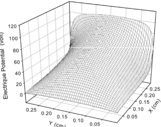
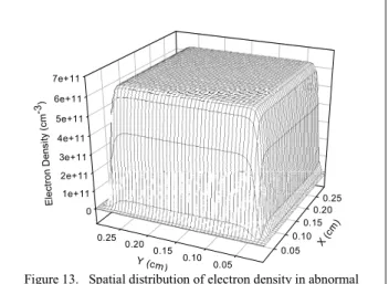
C. Abnormal glow discharge

To simulate the abnormal regime of the glow discharge we must obligatorily increase the source term and the applied voltage. We set S’=3.6×1017 (cm-3s-1), while the applied potential is to 120 V. This increase will involve a growth of the ionic and electronic density in the positive column.

The figures (13) to (16) show clearly the cathode and anode sheath and the positive column. The surface occupied by the positive column is very significant. This increase of the surface and the values of densities (6.3×1011 _cm-3_{) is due primarily at the source term and the} applied voltage. This expansion of the positive column leads automatically to the contraction of the cathode and anode sheath. 0 1e+11 2e+11 3e+11 4e+11 5e+11 6e+11 7e+11 0.05 0.10 0.15 0.20 0.25 0.05 0.10 0.15 0.20 0.25 E le ct ro n D en si ty ( cm -3) X (c m) Y (cm)

Figure 13. Spatial distribution of electron density in abnormal regime 0 1e+11 2e+11 3e+11 4e+11 5e+11 6e+11 7e+11 0.05 0.10 0.15 0.20 0.25 0.05 0.10 0.15 0.20 0.25 Io n D e ns ity ( cm -3 ) X (c m) Y (cm)

Figure 14. Spatial distribution of ion density in abnormal regime

We observe on figure (15) that the gradient of the potential in the cathode sheath becomes increasingly significant with the increase in the source term and the voltage applied.

The reduction of the cathode sheath is due to the expansion of the positive column, when the source term and the applied voltage increase

0 20 40 60 80 100 120 140 0.05 0.10 0.15 0.20 0.25 0.05 0.10 0.15 0.20 0.25 E le ct ri c po te n tia l (v ol t) X (c m) Y (cm)

Figure 15. Spatial distribution of electric potential in abnormal regime -8 -6 -4 -2 0 2 0.05 0.10 0.15 0.20 0.25 0.05 0.10 0.15 0.20 0.25 Lo ng itu di na l e le ct ric f ie ld ( kv c m -1) X(cm ) Y (cm)

Figure 16. Spatial distribution of longitudinal electric field in abnormal regime

-10 -8 -6 -4 -2 0 2 4 6 8 10 0.05 0.10 0.15 0.20 0.25 0.05 0.10 0.15 0.20 0.25 T ra n sv er se e le ct ric f ie ld ( kv c m -1) X(cm ) Y (cm)

Figure 17. Spatial distribution of transverse electric field in abnormal regime 0 1e+17 2e+17 3e+17 4e+17 5e+17 6e+17 7e+17 0.05 0.10 0.15 0.20 0.25 0.05 0.10 0.15 0.20 0.25 n et s o u rc e T e rm e ( cm -3 s -1 ) X(cm ) Y (cm)

Figure 18. Spatial distribution of source term in abnormal regime

It is noticed that the behavior of the axial field and the net source term in this regime is similar to those of the normal regime of the glow discharge.

The table II summarizes specific magnitude of electric grandeurs:

TABLE II: MAGNITUDE OF ELECTRIC GRANDEURS

Electric grandeurs

Subnormal regime

Normal regime Abnormal

regime S’ (cm-3_s-1) _8.0×1013 _3.6×1016 _3.6×1017 Va (V) 105 100 120 Vdiff (V) 0 6.22 5.05 ne (cm-3) 2.39×108 2.0×1011 6.39×1011 N+ (cm-3) 3.16×108 2.0×1011 6.39×1011 | EL| (V/cm) 643 4326 7512 Lg (mm) 0.62 0.25 0.03 xL (mm) . 0.51 0.4

The electric characteristics in a stationary state of different regimes of the glow discharge: Va, Vdiff, ne , n+,| EL|, Lg, xL, which are respectively anodic potential, difference between

maximal potential in the discharge and anodic potential (Vmax- Va), electronic and ionic densities, longitudinal field

at the cathode, sheath thickness and axial position where the longitudinal field becomes zero.

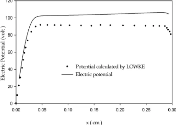
VII. VALIDITY TEST OF THE MODEL

To validate and test our numerical mode of resolution, we carried out a study of the discharge in argon, with the same conditions as the study of first order fluid model of authors Lowke and Davies [7]. We represent electron and ion density and electric potential distribution in figures (19) and (20). x (cm) 0.00 0.05 0.10 0.15 0.20 0.25 0.30 El ec tr on an d i on den si ties (c m -3) 0.0 5.0e+10 1.0e+11 1.5e+11 2.0e+11 2.5e+11

Electron density 1D and 2D code Ion density 1D and 2D code Electron density calculated by LOWKE Ion density calculated by LOWKE

Figure.19. Electronic and ionic densities spatial distribution given by Lowke and Davies and 2D code on symmetric axe

x ( cm ) 0.00 0.05 0.10 0.15 0.20 0.25 0.30 E lec tr ic Pot en tial (volt ) 0 20 40 60 80 100 120

Potential calculated by LOWKE Electric potential

Figure 20. Electric potential spatial distribution given by Lowke and Davies and 2D code on symmetric axe.

The electric proprieties results obtained for normal glow discharge in 1D code and 2D on symmetric axe [12], [13] are in good agreement with those obtained with Lowke and Davies 1D results.

IIX. CONCLUSION

In this paper, we presented a two-dimensional model of dc glow discharge in a Cartesian geometry. The charged particle kinetics is described with the first two moments of the equation of Boltzmann coupled with Poisson’s equation, assuming local equilibrium between particle kinetics and electric field. This 2D configuration made us possible to take into account the transverse

expansion of the glow discharge. This behavior is translated directly on the figures representing spatial distributions of the electronic and ionic densities, the potential and the transverse and longitudinal fields.

The results of simulation rest on the use of a stable and efficient implicit discretization scheme for the first two moments of the equation of Boltzmann.

An application of these numerical model results is used to describe the well-know properties of glow discharges and its different regime (subnormal, normal and abnormal regimes) and we note the influence of particle source and the applied potential. To validate the numerical method of resolution of the macroscopic equations, we studied the evolution of the glow discharge with the same conditions of Lowke and Davies [7].We note that the steady-state spatial distributions of the ion and electron densities and the electric potential on symmetric axe in 2D for normal glow discharge are in very good agreement with the results given by Lowke and Davies.

Further works are in progress where we develop a 1D and 2D numeric code considering the three moment of Boltzmann’s equation, with an electron diffusion and ionization frequency depending to electron energy, taking into account the approach of local average energy apply to the second order fluid model.

IX. REFERENCES

[1] L.E. Kline, in ‘”on equilibrium effects in ion and electron

transport”, Eds. J.W. Gallagher, D.F.Hudson, E.E. Kunhardt and R.J. Van Brunt, Plenum Press, New York p121, 1990

[2] A. Garscadden, Mat. Rev. Sco. Symp. Proc. Vol 165,

Materials Research Society, p3, 1990.

[3] A. Bogarts and R. Gijbels Computer Simulation of an

Analytical Direct Current Glow Discharge in Argon: Influence of the Cell Dimensions on the Plasma Quantities, J. Analytical Atomic Spectrometry, Vol. 12, p 751, 1997.

[4] J. P. Boeuf, and L.C. Pitchord, “ Pseudo spark discharges via

computer simulation “ IEEE Trans. On plasma Sci. 19(2), pp 286-296, 1991.

[5] computer simulation “ IEEE Trans. On plasma Sci. 19(2), pp

286-296, 1991.

[6] A. Hamid, A. Hennad and M. Yousfi “Modélisation d’une

décharge luminescente dans l’argon un terme source

constant”, 1rst _{Conférence Nationale Rayonnement –Matière}

CNRM1 19-20 Janvier 2003 p 64.

[7] D. Guendouz, A. Hamid, ‘’Electric characteristic of glow

discharge in 1D with constant source term’’, 6th _National

Conference of high Tension CNHT, special number of Algerian Journal of Technology AJOT, 46 :50, 2007.

[8] J. Lowke and K. Davies, J. Appl. Phys., 48, 4991, 1977.

[9] D. L. Scharfetter and H. K. Gummel, IEEE Trans. Electron

Devices ED-16, 64, 1969.

[10] J.P. Nougier "Méthodes de calcul numérique ", 2e _édition

Masson, Paris, 1985.

[11] S. Park and D. J. Economou, J. Appl. Phys., 68, 3904, 1990.

[12] C. B. Leffert, D. B. Rees, and F. E. Jamerson , J. .Appl.

Phys. 37, 133, 1966; J. W. Bong, in Radiation Dosimetry, edited by F. H. Attix and W. C. Roesch, (Academic, New York), Vol, II, Chap. 9, p.1, 1966.

[13] A. Hamid, A. Hennad and M. Yousfi “Modélisation

bidimensionnelle d’une décharge luminescente dans l’argon” VIII congrès Plasma de la Société Française de Physique SFP, CEA/Cadarache /France 5 - 7 may, 2003.

[14] D. Guendouz, A. Hamid, IREPHY, Vol 3 n. 5, 268: 273,