Improving the discrimination of primary and secondary sources of organic aerosol : use of molecular markers and different approaches

HAL Id: tel-01895752

https://tel.archives-ouvertes.fr/tel-01895752

Submitted on 15 Oct 2018

HAL is a multi-disciplinary open access archive for the deposit and dissemination of sci-entific research documents, whether they are pub-lished or not. The documents may come from teaching and research institutions in France or

L’archive ouverte pluridisciplinaire HAL, est destinée au dépôt et à la diffusion de documents scientifiques de niveau recherche, publiés ou non, émanant des établissements d’enseignement et de recherche français ou étrangers, des laboratoires

sources of organic aerosol : use of molecular markers and

different approaches

Deepchandra Srivastava

To cite this version:

Deepchandra Srivastava. Improving the discrimination of primary and secondary sources of organic aerosol : use of molecular markers and different approaches. Other. Université de Bordeaux, 2018. English. �NNT : 2018BORD0055�. �tel-01895752�

THÈSE PRÉSENTÉE POUR OBTENIR LE GRADE DE

DOCTEUR DE L’UNIVERSITÉ DE BORDEAUX ÉCOLE DOCTORALE DES SCIENCES CHIMIQUES

PREPAREE A

L’INSTITUT NATIONAL DE L’ENVIRONNEMENT INDUSTRIEL ET DES RISQUES (INERIS)

Par Deepchandra SRIVASTAVA

Improving the discrimination of primary and secondary sources of

organic aerosol: use of molecular markers and different approaches

Sous la direction de : Eric VILLENAVE

(co-direction de : Emilie PERRAUDIN) Soutenue le 26 avril 2018

Membres du jury :

Mme RIFFAULT Véronique, Professeure, IMT Lille-Douai Rapportrice M. WENGER John, Professeur, University College Cork, Ireland Rapporteur Mme D’ANNA Barbara, Directrice de recherche, LCE, Marseille Examinatrice Mme GROS Valerie, Directrice de recherche, LSCE Examinatrice

M. EL-HADDAD Imad, Chercheur, PSI Examinateur

M. ALBINET Alexandre, Ingénieur, INERIS Responsable de thèse

M. FAVEZ Olivier, Ingénieur, INERIS Responsable de thèse

Mme PERRAUDIN Emilie, Maître de conférences, Université de Bordeaux Co-encadrante de thèse M. VILLENAVE Eric, Professeur, Université de Bordeaux Directeur de thèse

The important thing is not to stop questioning.

Curiosity has its own reason for existing.

Les particules en suspension (ou aérosols) représentent aujourd’hui la classe de polluants atmosphériques la plus préoccupante en matière de santé publique et d’impact environnemental. De par la multiplicité de leurs sources d’émissions et/ou de leurs processus de formation dans l’atmosphère, elles ont une composition chimique complexe et leurs origines sont insuffisamment documentées. Une meilleure compréhension de ces phénomènes demeure essentielle à l’amélioration des outils de modélisation ainsi qu’à l’élaboration de politiques publiques efficaces.

Parmi les différentes familles de particules atmosphériques, les aérosols organiques (AO) font actuellement l’objet d’une attention particulière de la part de la communauté scientifique. Ils sont émis directement dans l’atmosphère (on parle alors d’AOP, pour aérosols organiques primaires), ou issus de processus de conversion gaz-particules (on parle alors d’AOS, pour aérosol organiques secondaires). AOP et AOS peuvent avoir des origines anthropiques ou biogéniques. L’objectif de ce travail de thèse était d’acquérir une meilleure connaissance de l’origine des AO à l’aide de marqueurs organiques moléculaires prélevés sur filtres et par couplage avec des données issues de mesures in-situ par spectrométrie de masse.

Une première étape de ce travail de thèse a consisté à réaliser une étude bibliographique sur les différentes approches d’étude de sources d’AO mises en œuvre au sein de la communauté internationale au cours des dix dernières années. Les méthodologies les plus souvent utilisées incluent les outils statistiques de type modèles récepteurs (e.g., Chemical Mass Balance (CMB) et Positive Matrix Factorization (PMF)), et les méthodes dites EC-tracer et SOA-tracer. Environ 200 études réalisées principalement en Europe, Amérique du Nord et Chine à l’aide de ces méthodologies ont pu être analysées et comparées. Chacune de ces méthodologies

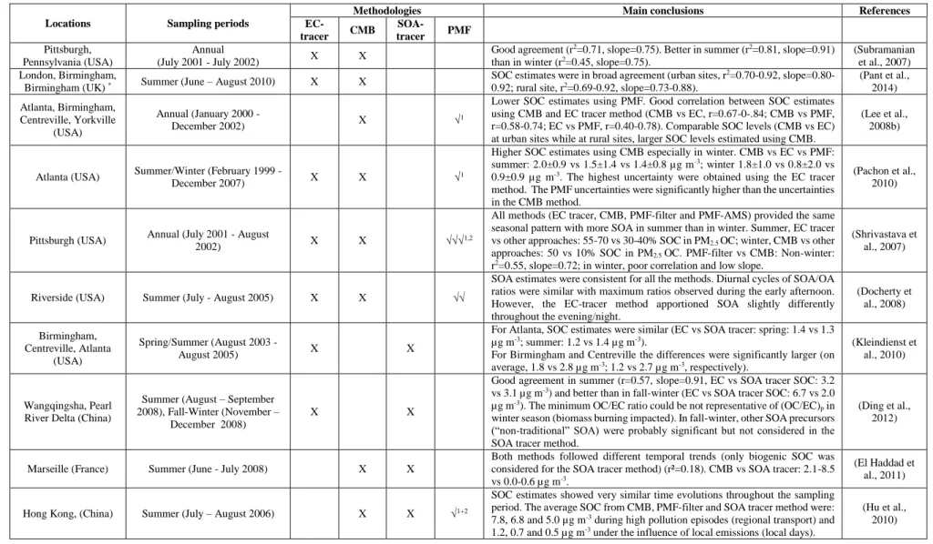
fraction organique des aérosols, en particulier lors de la période printemps-été (Figure 1). Des différences plus marquées sont observées en hiver, suggérant notamment la nécessité d’une meilleure prise en compte des émissions anthropiques liées à la combustion de biomasse (pour le chauffage). L’utilisation de nouveaux traceurs de sources moléculaires devraient permettre d’affiner la compréhension des phénomènes mis en jeux.

Figure 1: Comparaison de résultats présentés dans la littérature scientifique pour la

différenciation entre AOP et AOS au sein de la fraction fine des particules sur la période printemps-été (sites de fond urbain et péri-urbain) à l’aide des 4 méthodologies d’étude de sources les plus fréquemment utilisées en Europe, Amérique du Nord et Chine.

La deuxième étape de la thèse était donc focalisée sur l’analyse chimique aussi complète que possible d’échantillons représentatifs de deux milieux urbains français. Les jeux de données obtenus ont ensuite été exploités par application de la méthode PMF. Ce travail expérimental a été basé sur deux campagnes de prélèvements réalisées à Grenoble (site urbain) au cours de

caractérisation chimique étendue (de 139 à 216 espèces quantifiées) a été réalisée et l’utilisation de marqueurs moléculaires primaires et secondaires clés dans la PMF a permis de déconvoluer de 9 à 11 sources différentes de PM10 (respectivement à Grenoble et au SIRTA, Figures 2 et 3) incluant aussi bien des sources classiques (combustion de biomasse, trafic, poussières, sels de mer, nitrate et espèces inorganiques secondaires) que des sources non communément résolues telles que AO biogéniques primaires (spores fongiques et débris de plantes), AO secondaires (AOS) biogéniques (marin, oxydation de l’isoprène) et AOS anthropiques (oxydation des hydrocarbures aromatiques polycycliques (HAP) et/ou des composés phénoliques). En outre, le jeu de données obtenu pour la région parisienne à partir de prélèvements sur des pas de temps courts (4 h) a permis d’obtenir une meilleure compréhension des profils diurnes et des processus chimiques impliquées.

Figure 2: Contributions moyennes (à gauche) et évolutions temporelles (à droite) des différents

facteurs de sources de l’AO identifiés par PMF pour le site de fond urbain de Grenoble au cours de l’année 2013.

Figure 3. Contributions moyennes (à gauche) et évolutions temporelles (à droite) des différents

facteurs de sources de l’AO identifiés par PMF pour le site de fond péri-urbain du SIRTA lors de l’épisode de pollution aux particules de mars 2015.

Les résultats obtenus pour le site du SIRTA ont pu être comparés à ceux issus d’autres techniques de mesures (en temps réel, ACSM (aerosol chemical speciation monitor) et analyse AMS (aerosol mass spectrometer) en différée) et/ou d’autres méthodes de traitement de données (méthodes traceur EC (elemental carbon) et traceur AOS). Un bon accord a été obtenu entre toutes les méthodes en termes de séparation des fractions primaires et secondaires (Figures 4 et 5).

L’identification des facteurs liés aux émissions primaires du trafic et de la combustion de biomasse a été confirmée par leurs profils diurnes. Ceux-ci sont comparables d’une méthodologie à l’autre avec cependant quelques problèmes de mélange dans le cas des analyses PMF basées sur les spectres de masse aérosol. Pour les facteurs AOS individuels, le facteur mélange d’aérosols secondaires obtenu à partir de la PMF appliquée sur les données chimiques filtres montre une très bonne corrélation avec les facteurs AO très oxydés déterminés à partir des analyses des données de spectrométrie de masse aérosol. Ces résultats suggèrent une origine commune de ces facteurs.

Figure 4: Comparaison des concentrations totales carbone organique primaire (POC)

estimées à partir de différentes méthodologies. A (figure du haut) : séries temporelles. B (figures du bas) : Boites à moustaches indiquant la valeur minimum, le premier quantile, la valeur médiane, le troisième quantile et la valeur maximum. POC*PMF-chemical data: PMF basée sur les données chimiques filtres sans la part issus des poussières ; POC*PMF-offline AMS: PMF basée sur les données offline AMS sans le facteur SCOA.

Figure 5: Comparaison des concentrations totales en carbone organique secondaire (SOC)

mécanismes spécifiques de formation et/ou des précurseurs gazeux responsables de cette fraction de l’AOS (qui représente ici environ 25% de l’AO total dans les PM10). En particulier, pour la méthode SOA-tracer, même si la contribution secondaire de la combustion de biomasse a été prise en compte, la quantité totale d’AOS observée lors de l’épisode de pollution à longue distance est largement sous-estimée probablement en lien avec des espèces non prises en compte telles que les organonitrates ou organosulfates.

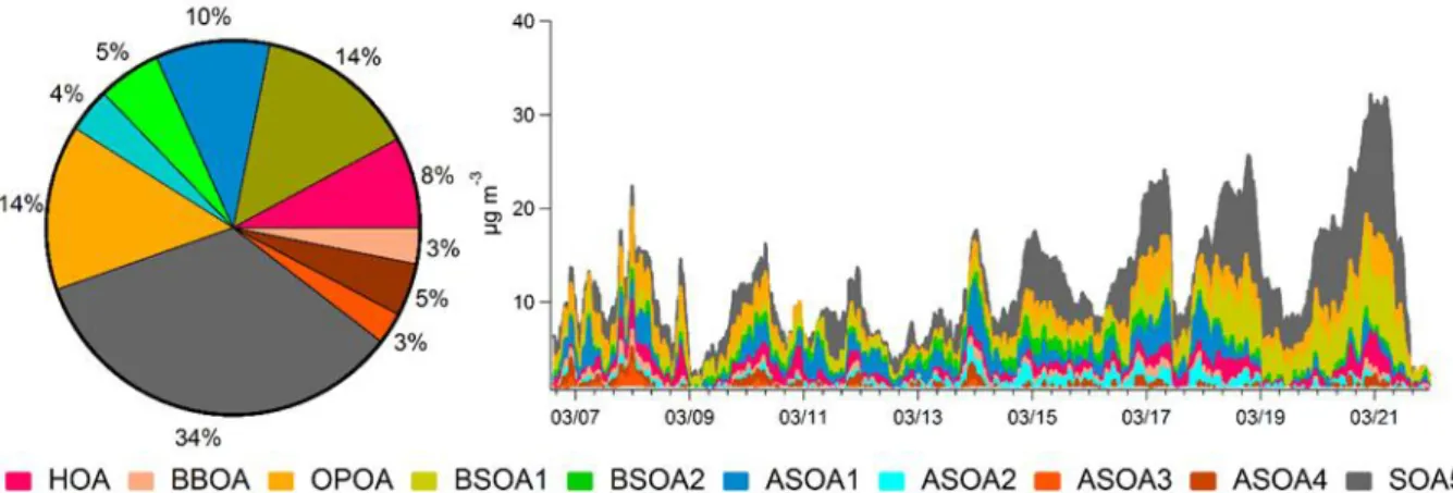
Ainsi, une nouvelle approche d’étude des sources de l’AO a été développée en combinant les mesures en temps réel (ACSM) et celles sur filtres (marqueurs moléculaires organiques) et en utilisant un script de synchronisation des données. Cette méthodologie a été appliquée aux données issues de la campagne réalisée en mars 2015 au SIRTA. L’analyse PMF combinée a été mise en œuvre sur la matrice de données unifiée, conduisant à l’obtention de 10 facteurs de source d’AO, dont 3 facteurs primaires et 7 facteurs secondaires (Figure 6). La cohérence de cette nouvelle méthodologie a été étudiée en comparant les résultats obtenus avec ceux issus de l’analyse PMF des données ACSM. Les résultats montrent une très bonne concordance pour les deux fractions, primaires et secondaires. Cette nouvelle méthode a permis l’identification claire de près de la moitié de la masse totale d’AOS (75% de OA) observée au cours de la campagne de prélèvements. Les facteurs secondaires identifiés ont été classés selon leur état d’oxydation, sources et/ou précurseurs d’AOS. Au final, environ 28% de la fraction totale semble liée à l’AOS anthropique (4 facteurs AOS) en lien avec les sources de combustion telles que la combustion de biomasse et les émissions issues du trafic routier.

Figure 6: Contributions moyennes (gauche) et évolution temporelle (droite) des différentes

sources d’AO identifiées à Paris-SIRTA, France (Mars 2015). HOA : émissions primaires trafic ; BBOA : combustion de biomasse OA ; OPOA : AO primaire oxydé; BSOA-1 : AOS biogénique 1 (marin enrichi); BSOA-2 : AOS biogénique 2 (oxydation de l’isoprène); ASOA-1 : AOS anthropique 1 (HAP oxygénés) ; ASOA-2 : AOS anthropique 2 (HAP nitrés) ; ASOA-3: AOS anthropique 3 (oxydation des composés phénoliques); ASOA-4 : AOS anthropique 4 (oxydation du toluène) et SOA-5 (AOS 5).

Les résultats obtenus ont aussi mis en évidence que 4 facteurs AO étaient liés aux émissions de la combustion de biomasse avec 2 sources primaires (AO combustion de biomasse (BBOA) et AOP oxydé (OPOA)) et 2 facteurs secondaires (en lien avec l’oxydation des composés phénoliques et du toluène). Chose intéressante, 80% du BBOA primaire semble être en fait de l’OPOA. L’AOS anthropique lié à l’oxydation des HAP (caractérisé par les nitro-HAP), toluène et les composés phénoliques, a montré des variations diurnes particulières avec des fortes concentrations au cours de la nuit indiquant un rôle majeur de la chimie nocturne. L’établissement d’un lien direct entre MO-OOA (OA oxygéné plus oxydé) ou LO-OOA (OA oxygéné moins oxydé), issus de l’analyse PMF des données ACSM, avec une source donnée est finalement très difficile à faire. Les résultats obtenus ont montré que l’OOA plus oxydé est probablement associé à des sous-produits d’oxydation ultimes alors que l’OOA moins oxydé

compréhension des processus chimiques liés aux différentes sources de l’AO.

Mots clés : Chimie atmosphérique, Aérosols organiques, Marqueurs moléculaires, Positive

First and foremost, I would like to acknowledge my sincere gratitude to Alex, Olivier, Eric and Emilie for giving me the opportunity to pursue my dreams. My most special thanks go to Alex and Olivier, with whom I have learnt all the new aspects of atmospheric sciences. Our trips to conferences, workshops and meeting, and long discussions (with 100+ slides) not have only helped me to evolve as a good researcher but their constant aid and suggestions have given me courage to believe and present myself in a better way. My list of questions has never bothered them, on the contrary they have always appreciated my curiosity. I would like to thank both for guarding each step of my career in the last years, and helping me to discover new things. The point where I have reached today in my career it would have not been possible without their guidance and unparalleled support, thank you so much for everything (from prefecture to articles). My sincere thanks also go to Eric and Emilie, for their thoughtful suggestions and discussions on skype, have helped me to learn something new always. The knowledge I got over our discussions and support during the China trip with Eric, was unforgettable, that has helped me to learn more about my field, thanks a lot. I would also like to thank Eric for taking care of the things at the university. I am also thankful to Emilie for sharing some good discussions during EAC and PhD day at Bordeaux and email exchanges we had. I would also like to give thanks to the members of the jury for agreeing to judge this work in a limited time. I am really thankful to Véronique RIFFAULT, John WENGER, Barbara D’ANNA, Valerie GROS, and Imad EL-HADDAD for their remarks, corrections, kindness and the exchanges that we had.

I am also very thankful to Kaspar and Imad for their help for the offline AMS analyses. The support I received especially from Kaspar to understand offline AMS data was incredible. Kaspar’s constant help and input to make me understand the different stages of the offline AMS

mystery behind some unresolved things (i.e. WSOC). I also wanted to thank Dr. Philip K. Hopke, Uwayemi Sofowote and Jean-Eudes Petit (J-E) for their remarkable help in the understanding of ME-2 script. The discussions linked to error calculation, application of the constraints, and many more.., kept the research flow to move smoothly and never allowed stress to win over. I wanted to especially thank J-E, without whom this ME-2 work should not have reached to its final stage. Our discussion over ME-2, his warm hospitality in Reims, and ZeFir graphs (still feel they are the hottest ones), and PMF discussions (long running chapter), everything was amazing.

I would also like to thank the people from the lab (RESA). Firstly, a special and big thanks to Jérôme, without whom my GC analysis could have never happened, his constant support and lessons have made my GC path easier. Also, he never got bored with my questions, and the troubles I often had while running GC. The training he provided me on the sample preparation, sample analysis, troubleshooting, everything linked to instrumentation, have helped to set up a solid base for my analytical knowledge what I own today. Secondly, Francois, it was always delightful to have discussion with him. I still remember when I had a lot of issue related to TDU, he often used to come to discuss. Third one goes to Herve, Claudine, Nicolas, Serguei, Faustina, Jean-Pierre, Azziz and Ahmad, thank you so much for helping me out always. I would like to thank people from my building, Florence, Jean, Sabastien, Anne-Sophie, Aline, Jessica, Valerie, Marie, Cecile, Nathalie, Celine, Benedicte, Nathalie, Robin, Vincent, Sylvie, Fabrice, Marion, Serge, Warda and Isaline. With all of them I never felt that I am living thousand miles away from home, every morning was wonderful in the lab including delicious cakes upstairs sometimes, thank you everyone. I particularly would like to thank Francois Gautier, the information provided by him on French culture has made my stay amicable. I would

administrative purposes, for taking care of the things which was not always easy.

I would like to thank Tanguy, first friend of mine, I think I can say that after my arrival in France. Our discussions on science, politics (European + South China sea + US), religions and philosophy have really broadened my views on both aspects science as well as on social side. I am also good in football and Rugby now, ops not in playing just for the knowledge because of our discussions. I would also like to say thank to Patric Bodu for his support for all the graphical abstracts, all of them are simply great. I am also thankful to Florian for some nice discussions on SOA formation.

My heartily thanks for the members of my office, Yunjiang and Grazia. The time I had in my office it was beyond expectation, it was amazing. Discussions on ACSM datasets with Yunjiang and chemistry with Grazia, were always overwhelming, and helped further to enhance my basics on the things which I was not aware so much before. Apart from that, our funny chats over the topics where we had to explain to Yunjiang always, have also increased my humour as I was very bad in that initially. I am really thankful to you guys for being there through the highs and lows of PhD life. I am also thankful to Camille, new member of my office, successor of my office desk, her delightful nature and wonderful smile, have kept my stress level at the bottom during the last months of thesis.

I would like to thank Helene and Daniel, for making my life easier in France and for sharing some good time together. Thank you so much for dealing with all the letters and emails I received as my French level was initially zero. Apart from that, thank you Daniel for telling me about the things in the lab during my initial days and Helene for showing me the fish brain for the first time, and teaching me French in the starting days during lunch at the canteen. A big thanks to my group of friends, those have given some charm and cherish memories to my PhD

to Anitha for good Indian food and some nice evenings. I would never forget our trip to Fécamp (3 GB of pictures in 3 days), Amiens (dancing **), Brussels (Yunjiang*), Switzerland (coca cola project invention), and many more, thank you so much for giving the opportunity to have a balanced work life. I would also like to thank Julie, Julien, Vincent, Marta, Martin, Valentin, Clemence, Quentin, Ibtihel and Victor for sharing some good time together. Thank you so much guys, for the madness, and the good moments whether in the lab or outside we shared. A big thanks to all the other people at INERIS, including people at canteen, accueil, bibliothèque, DSI, ECOT lab, and Christine Couverchel for their generous behaviour and help.

I am also thankful to Sophie for the friendship, the good times we shared on skype to discuss about Iron Man (Grenoble Fe conc.), her unconditional support for everything whether it is linked to papers, PhD manuscript, PAHs or on GC unconventional problems. I am pretty sure Google is going to complain for our long Gmail chats. I am also thankful to Julien from Bordeaux for the good time we had in China.

My PhD journey is incomplete without acknowledging my family, their everlasting support, faith and unconditional love, have given me the inspiration to live my passion, my work. Even I am so far from the home but they never let me think a bit of it, my passion is more important for them rather than the distance, thank you so much for having immense trust on me. I am also thankful to my friends from India and abroad for their support since last couple of years. Then there are some fictional characters, without them I don’t think I can survive. Thank you so much Sheldon, Sherlock, Michael Scolfield, Dr. House and Mr. Robot, you guys were always there and made me happy as much as you can. Finally, at last I would like to thank my laptops (LP-1003171 & LB-1004604), I know we were good companions, and we proved it at the end bravo!!.

Chapter I: General introduction and objectives of the Thesis ... 1

1.1. Context ... 3

1.2. Objectives of the PhD Thesis ... 9

1.3. Strategy of the PhD Thesis and organization of the manuscript ... 9

Chapter II: State of the art of SOA estimation methodologies ... 15

Comparison of methodologies based on measurement data to apportion Secondary Organic Carbon (SOC) in PM2.5: a review of recent studies Article I ... 17

Supplementry Material of Article I. ... 115

Chapter III: Experimental section ... 151

3.1. Sampling sites ... 153

3.2. Sampling periods and sample collection ... 155

3.3. On line measurements ... 157

3.4. Chemical Characterization ... 159

3.4.1. Analytical procedures ... 159

3.4.2. PAHs and their derivatives ... 162

3.4.3. Analysis of SOA markers ... 169

3.5. Chemical Mass Closures ... 175

Chapter IV: Speciation of organic fraction does matter for source apportionment ... 185

Speciation of organic fraction does matter for source apportionment. Part 1: a one-year campaign in Grenoble (France) Article II ... 187

Supplementry Material of Article II ... 203

Speciation of organic fractions does matter for aerosol source apportionment. Part 2: intensive short-term campaign in the Paris area (France) Article III ... 237

Supplementry Material of Article III ... 251

Chapter V: Comparison of different POA and SOA estimation methodologies ... 287

Comparison of different methodologies to discriminate between primary and secondary organic aerosols Article IV ... 289

organic aerosols fractions

Article V ... 345

Supplementry Material of Article V ... 385

Chapter VII: Conclusions and perspectives ... 405

Chapter I

General introduction and objectives of the

Thesis

1.1. Context

The impact of particulate matter (PM) on air quality, and so on human health, is now well recognized. A growing number of studies are notably confirming its influence on the occurrence of respiratory and cerebrovascular diseases, as well as heart attacks and other cardiovascular issues (Kelly and Fussell, 2015; Lippmann et al., 2013; Quan et al., 2010). The implementation of action plans to accurately reduce PM concentration levels in ambient air relies on sound knowledge of their origins. However, the scientific community and public powers are still facing PM source apportionment issues due to the multiplicity of their emission sources and the complexity of their (trans)-formation processes in the atmosphere.

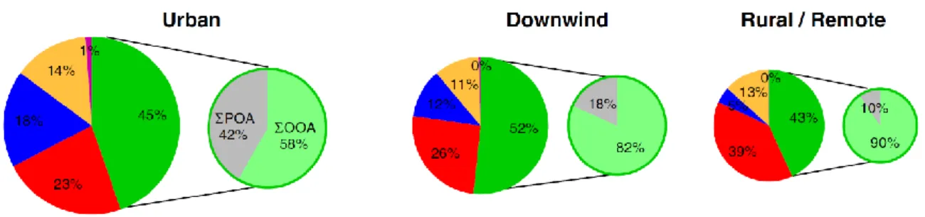
Within the complex airborne particle mixture, organic matter represents a large fraction of the total mass of fine aerosols (from 20 to 90 % in the low troposphere) (Kanakidou et al., 2005; Kroll and Seinfeld, 2008). Organic aerosols (OA) also correspond to the most challenging and ambiguous chemical species in terms of molecular composition, sources, and formation processes. As other atmospheric particles, OA are commonly distinguished according to their introduction mode in the particulate phase. Organic compounds directly emitted in the particulate phase in ambient air are defined as primary organic aerosol (POA). Particulate organic species originating from the oxidation reactions of (semi-) volatile organic compounds (VOCs, SVOCs) and mass transfer processes of their by-products into the aerosol, either via homogeneous or heterogeneous mechanisms, form the secondary organic aerosol (SOA) (Hallquist et al., 2009). The distribution between POA and SOA strongly depends on the location and the season. If POA emissions could eventually be controlled once elucidated, SOA, influenced by biogenic/anthropogenic VOC emissions and by atmospheric photochemistry, are more difficult to regulate. A better knowledge on their origins are though fundamental as they

may constitute about 80 to 90 % of the total OA in some locations (Carlton et al., 2009; Zhang et al., 2011) (Figure I.1).

Figure I.1. Average PM1 composition. Pink: chloride; Yellow: ammonium, Blue: nitrate; Red: sulfate; Green: organic; Light green: oxygenated organic aerosol (OOA); Grey: primary organic aerosol (POA). Adapted from Zhang et al. (2011).

A better understanding of OA sources and/or their formation processes is also crucial for the optimization of chemistry-transport models which are still commonly unable to accurately simulate various OA fractions, and especially SOA (Ciarelli et al., 2016) (Figure I.2).

Such issues of current models notably lead to a poor air quality forecast during specific pollution events, such as those related to high loadings of biomass burning emissions. They also participate to significant uncertainties within near-term climate models, which do not fully take OA into account (Belis et al., 2013).

Epidemiological studies show a clear link between increased mortality and enhanced concentrations of ambient aerosols. The chemical and physical properties of aerosol particles causing health effects are still unclear. Recent studies have shown that a significant amount of SOA (major fraction of OA as shown before) may induce potential health risk (Baltensperger et al., 2008; Kramer et al., 2016; Tuet et al., 2017). Particularly, PAHs (polycyclic aromatic hydrocarbons) derivatives (oxy- and nitro-PAHs) are probably more mutagenic than their

parent PAHs as they act as direct mutagens (Baltensperger et al., 2008; Durant et al., 1996; Kramer et al., 2016; Pedersen et al., 2005; Rosenkranz and Mermelstein, 1985; Tuet et al., 2017). Furthermore, some of these compounds are suspected to be carcinogenic and have been recently classified in the 2A (probably carcinogenic to human) and 2B (possibly carcinogenic to human) groups by IARC (International Agency for Research on Cancer, IARC, 2013, IARC, 2012). Therefore, investigating the sources of such compounds can be a key tool to assess health risks for humans exposed to airborne pollutants.

Figure I.2. Comparison of OA simulation by three currently used European Chemistry

Transport Models to measurements at a Swiss rural background site in March 2009 and June 2006. Adapted from Ciarelli et al. (2016).

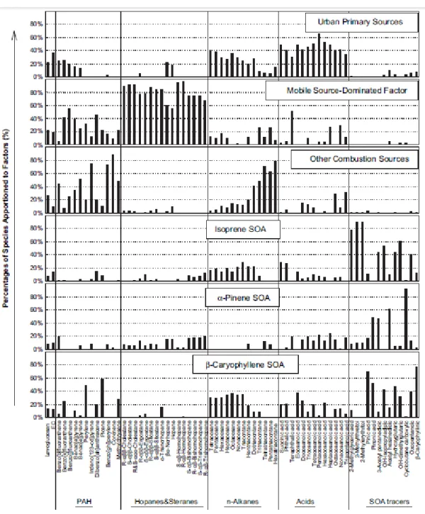
Several source apportionment methodologies have been developed during the last decades. These methods are generally based on the monitoring data, emission inventories (i.e., dispersion models) and statistical evaluations (i.e., receptor models)(Gray et al., 1986; Grosjean, 1984; Kleindienst et al., 2007; Paatero, 1997; Paatero and Tapper, 1994; Turpin and Huntzicker, 1995; Watson et al., 1990). However, only few of these approaches (e.g., SOA-tracer method, positive matrix factorization (PMF)) can provide direct information on the secondary sources based on the chemical speciation of molecular markers (Kleindienst et al., 2007; Kleindienst et al., 2010; Shrivastava et al., 2007; Zhang et al., 2009). The latter species should have a high degree of source specificity and be relatively stable in the atmosphere, to allow gaining insights into aerosol sources and the underlying mechanisms of SOA formation and/or ageing (Schauer et al., 1996). Recently, considerable progress has been made in the molecular characterization of individual SOA constituents from the photooxidation of biogenic and anthropogenic VOCs that can serve as markers for SOA characterization, such as markers from isoprene oxidation, 2- methyltetrols (i.e., the diastereoisomers, methylthreitol and methylerythritol) and 2-methylglyceric acid. These markers have already been used in receptor models (i.e., PMF) to provide deep insight into OA fractions (Heo et al., 2013; Hu et al., 2010; Jaeckels et al., 2007; Shrivastava et al., 2007; Zhang et al., 2009). It appears that the use of molecular markers has the unique advantage of distinguishing SOA contributions from different VOC precursor classes (Figure I.3). Filter-based markers often rely on rather weak time-resolution (typically 24 h), making it difficult to isolate fast transformation processes. Thus, there are still significant gaps in our knowledge which places limitations on our ability to investigate SOA origins.

Figure I.3. Distribution of molecular markers among identified factors in OA source

apportionment using PMF model. Adapted from Zhang et al. (2009).

On the other hand, for about 15 years, the use of online instrumentation for aerosol chemical characterization (i.e., AMS (aerosol mass spectrometer), ACSM (aerosol chemical speciation monitor)) has successfully improved the real-time measurements of particulate organic

OA factors (Lanz et al., 2007; Ulbrich et al., 2009; Zhang et al., 2011). The evolution of OA in the atmosphere is assessed to follow progressive oxidation steps from fresh to highly aged OA associated with a change of chemical functionalities, volatility, and oxidation state (Ng et al., 2010; Sun et al., 2011). The various OA factors retrieved from PMF analysis are then differentiated according to these properties, which might be roughly attributed to either primary or secondary fractions. However, such a discrimination remains relatively uncertain due to the non-specific nature of the measured mass fragments.

In this context, scientific efforts have still to be undertaken to get a better understanding of OA origins, considering as far as possible the whole complexity and variability of the involved processes. Combining different datasets from several measurement set-ups to refine the source apportionment of OA, and notably secondary ones, might help to achieve this goal.

1.2. Objectives of the PhD Thesis

The main goal of this experimental PhD work is to investigate methodologies dedicated to the source apportionment of POA and SOA fractions. These objectives can be described according to the three following questions:

1) How well does current and commonly-used OA source apportionment approaches agree to each other?

2) Which “novel” organic molecular markers could help a better discrimination between primary/secondary and/or biogenic/anthropogenic origins?

3) Can we improve the data treatment of OA mass spectra using some of these specific markers?

1.3. Strategy of the PhD Thesis and organization of the manuscript

To achieve these objectives, the present work has been designed in four main steps:

The first step involved a review on the different approaches currently used to apportion SOA fractions. Here, it has been chosen to mainly focus on SOA, rather than POA, as this fraction is probably the most challenging and is currently subject to on-going methodological developments. Benefits as well as drawbacks and specific issues of the considered approaches are discussed and compared. This review also offered the opportunity to summarise results obtained from a large set of studies conducted in different regions across the world.

The second step included the chemical analysis of a wide variety of molecular organic markers, notably including primary and secondary PAHs, anhydrosugars, cellulose combustion products, odd number higher alkanes, methanesulfonic acid (MSA), and various SOA markers related to the oxidation of isoprene, α-pinene, toluene, and phenolic compounds. These measurements were performed on filter samples collected during two field campaigns: a one year (2013)

campaign at a background urban site in Grenoble (France, Alpine region), and a short-term intensive campaign conducted in the Paris area at SIRTA during a PM pollution event (March 2015). Both of these datasets were enriched with inorganic and metallic species measurements, and then subjected to PMF analysis.

The third step corresponded to the comparison of results obtained from various source apportionment approaches (namely, PMF, EC- tracer method, and SOA-tracer method) applied to different datasets (extended chemical data, ACSM measurements, and offline AMS analysis) obtained from the intensive Paris campaign.

The fourth step relied on an attempt to develop a novel source apportionment methodology to refine the understanding of the various OA sources. In this last step, PMF was carried out with time synchronization using the multilinear engine (ME-2) algorithm on the combined dataset including OA ACSM mass spectra and specific primary and secondary organic molecular markers.

The plan of the present manuscript is basically following the order of these steps, half of the chapters being directly presented in the form of articles already published, or to be submitted soon. The next (and second) chapter is devoted to the review paper dedicated to commonly and widely used SOA source apportionment approaches (Article I). The third chapter describes the experimental work conducted during this thesis, including information on sampling sites, on the used instrumentation, and on the procedures developed/ improved for the analysis of organic molecular markers. The fourth chapter presents the results linked to the use of key organic molecular markers into PMF analysis applied to the Grenoble and Paris datasets (Articles II and III). The fifth chapter corresponds to the article related to the comparison of results obtained from different common methodologies applied to the Paris datasets (Article IV). The sixth chapter deals with the development of a synergic approach to refine OA source

apportionment by combining off-line and on-line measurements (Article V). Finally, the seventh chapter corresponds to major conclusions and perspectives linked to this work.

Due to the structure of this manuscript and the inclusion of articles already submitted or nearly submitted to different journals, references are separately provided in a dedicated subsection within each chapter.

References

Baltensperger, U., Dommen, J., Alfarra, M. R., Duplissy, J., Gaeggeler, K., Metzger, A., Facchini, M. C., Decesari, S., Finessi, E., Reinnig, C., Schott, M., Warnke, J., Hoffmann, T., Klatzer, B., Puxbaum, H., Geiser, M., Savi, M., Lang, D., Kalberer, M., Geiser, T., 2008. Combined determination of the chemical composition and of health effects of secondary organic aerosols: the POLYSOA project. J Aerosol Med Pulm Drug Deliv. 21, 145-54.

Belis, C. A., Karagulian, F., Larsen, B. R., Hopke, P. K., 2013. Critical review and meta-analysis of ambient particulate matter source apportionment using receptor models in Europe. Atmos. Environ. 69, 94-108.

Carlton, A. G., Wiedinmyer, C., Kroll, J. H., 2009. A review of Secondary Organic Aerosol (SOA) formation from isoprene. Atmos. Chem. Phys. 9, 4987-5005.

Ciarelli, G., Aksoyoglu, S., Crippa, M., Jimenez, J.-L., Nemitz, E., Sellegri, K., Äijälä, M., Carbone, S., Mohr, C., O'Dowd, C., 2016. Evaluation of European air quality modelled by CAMx including the volatility basis set scheme. Atmos. Chem. Phys. 16, 10313-10332.

Durant, J. L., Busby, W. F., Lafleur, A. L., Penman, B. W., Crespi, C. L., 1996. Human cell mutagenicity of oxygenated, nitrated and unsubstituted polycyclic aromatic hydrocarbons associated with urban aerosols. Mutation Research/Genetic Toxicology. 371, 123-157.

Gray, H. A., Cass, G. R., Huntzicker, J. J., Heyerdahl, E. K., Rau, J. A., 1986. Characteristics of atmospheric organic and elemental carbon particle concentrations in Los Angeles. Environ. Sci. Technol. 20, 580-589.

Grosjean, D., 1984. Particulate carbon in Los Angeles air. Sci. Total Environ. 32, 133-45. Hallquist, M., Wenger, J., Baltensperger, U., Rudich, Y., Simpson, D., Claeys, M., Dommen,

J., Donahue, N., George, C., Goldstein, A., 2009. The formation, properties and impact of secondary organic aerosol: current and emerging issues. Atmos. Chem. Phys. 9, 5155-5236.

Heo, J., Dulger, M., Olson, M. R., McGinnis, J. E., Shelton, B. R., Matsunaga, A., Sioutas, C., Schauer, J. J., 2013. Source apportionments of PM2.5 organic carbon using molecular marker Positive Matrix Factorization and comparison of results from different receptor models. Atmos. Environ. 73, 51-61.

Hu, D., Bian, Q., Lau, A. K. H., Yu, J. Z., 2010. Source apportioning of primary and secondary organic carbon in summer PM2.5 in Hong Kong using positive matrix factorization of secondary and primary organic tracer data. J. Geophys. Res.-Atmos. 115,

IARC, 2012. Some Chemical Present in Industrial and Consumer Products, Food and

Drinking-Water Vol. 101 (868 pp.

https://monographs.iarc.fr/ENG/Monographs/vol101/mono101.pdf).

IARC, 2013. Diesel and Gasoline Engine Exhausts and Some Nitroarenes Vol. 105 (714 pp.https://monographs.iarc.fr/ENG/Monographs/vol105/mono105.pdf).

Jaeckels, J. M., Bae, M.-S., Schauer, J. J., 2007. Positive matrix factorization (PMF) analysis of molecular marker measurements to quantify the sources of organic aerosols. Environ. Sci. Technol. 41, 5763-5769.

Kanakidou, M., Seinfeld, J., Pandis, S., Barnes, I., Dentener, F., Facchini, M., Dingenen, R. V., Ervens, B., Nenes, A., Nielsen, C., 2005. Organic aerosol and global climate modelling: a review. Atmos. Chem. Phys. 5, 1053-1123.

Kelly, F. J., Fussell, J. C., 2015. Air pollution and public health: emerging hazards and improved understanding of risk. Environ. Geochem. Health. 37, 631-649.

Kleindienst, T. E., Jaoui, M., Lewandowski, M., Offenberg, J. H., Lewis, C. W., Bhave, P. V., Edney, E. O., 2007. Estimates of the contributions of biogenic and anthropogenic hydrocarbons to secondary organic aerosol at a southeastern US location. Atmos. Environ. 41, 8288-8300.

Kleindienst, T. E., Lewandowski, M., Offenberg, J. H., Edney, E. O., Jaoui, M., Zheng, M., Ding, X., Edgerton, E. S., 2010. Contribution of Primary and Secondary Sources to Organic Aerosol and PM2.5 at SEARCH Network Sites. J. Air Waste Manage. Assoc. 60, 1388-1399.

Kramer, A. J., Rattanavaraha, W., Zhang, Z., Gold, A., Surratt, J. D., Lin, Y.-H., 2016. Assessing the oxidative potential of isoprene-derived epoxides and secondary organic aerosol. Atmos. Environ. 130, 211-218.

Kroll, J. H., Seinfeld, J. H., 2008. Chemistry of secondary organic aerosol: Formation and evolution of low-volatility organics in the atmosphere. Atmos. Environ. 42, 3593-3624. Lanz, V. A., Alfarra, M. R., Baltensperger, U., Buchmann, B., Hueglin, C., Szidat, S., Wehrli, M. N., Wacker, L., Weimer, S., Caseiro, A., 2007. Source attribution of submicron organic aerosols during wintertime inversions by advanced factor analysis of aerosol mass spectra. Environ. Sci. Technol. 42, 214-220.

Lippmann, M., Chen, L., Gordon, T., Ito, K., Thurston, G., 2013. National Particle Component Toxicity (NPACT) Initiative: integrated epidemiologic and toxicologic studies of the health effects of particulate matter components. Research Report (Health Effects Institute). 5-13.

Ng, N. L., Canagaratna, M. R., Zhang, Q., Jimenez, J. L., Tian, J., Ulbrich, I. M., Kroll, J. H., Docherty, K. S., Chhabra, P. S., Bahreini, R., Murphy, S. M., Seinfeld, J. H., Hildebrandt, L., Donahue, N. M., DeCarlo, P. F., Lanz, V. A., Prévôt, A. S. H., Dinar, E., Rudich, Y., Worsnop, D. R., 2010. Organic aerosol components observed in Northern Hemispheric datasets from Aerosol Mass Spectrometry. Atmos. Chem. Phys. 10, 4625-4641.

Paatero, P., 1997. Least squares formulation of robust non-negative factor analysis. Chemom. Intell. Lab. Syst. 37, 23-35.

Paatero, P., Tapper, U., 1994. Positive matrix factorization: A non‐negative factor model with optimal utilization of error estimates of data values. Environmetrics. 5, 111-126.

Pedersen, D. U., Durant, J. L., Taghizadeh, K., Hemond, H. F., Lafleur, A. L., Cass, G. R., 2005. Human Cell Mutagens in Respirable Airborne Particles from the Northeastern United States. 2. Quantification of Mutagens and Other Organic Compounds. Environ. Sci. Technol. 39, 9547-9560.

Quan, C., Sun, Q., Lippmann, M., Chen, L.-C., 2010. Comparative effects of inhaled diesel exhaust and ambient fine particles on inflammation, atherosclerosis, and vascular dysfunction. Inhalation Toxicol. 22, 738-753.

Rosenkranz, H. S., Mermelstein, R., 1985. The genotoxicity, metabolism and carcinogenicity of nitrated polycyclic aromatic hydrocarbons. Journal of Environmental Science and Health. Part C: Environmental Carcinogenesis Reviews. 3, 221-272.

Schauer, J. J., Rogge, W. F., Hildemann, L. M., Mazurek, M. A., Cass, G. R., Simoneit, B. R., 1996. Source apportionment of airborne particulate matter using organic compounds as tracers. Atmos. Environ. 30, 3837-3855.

Shrivastava, M. K., Subramanian, R., Rogge, W. F., Robinson, A. L., 2007. Sources of organic aerosol: Positive matrix factorization of molecular marker data and comparison of results from different source apportionment models. Atmos. Environ. 41, 9353-9369. Sun, Y. L., Zhang, Q., Schwab, J. J., Demerjian, K. L., Chen, W. N., Bae, M. S., Hung, H. M.,

Hogrefe, O., Frank, B., Rattigan, O. V., Lin, Y. C., 2011. Characterization of the sources and processes of organic and inorganic aerosols in New York city with a high-resolution time-of-flight aerosol mass apectrometer. Atmos. Chem. Phys. 11, 1581-1602.

Tuet, W. Y., Chen, Y., Xu, L., Fok, S., Gao, D., Weber, R. J., Ng, N. L., 2017. Chemical oxidative potential of secondary organic aerosol (SOA) generated from the photooxidation of biogenic and anthropogenic volatile organic compounds. Atmos. Chem. Phys. 17, 839-853.

Turpin, B. J., Huntzicker, J. J., 1995. Identification of secondary organic aerosol episodes and quantitation of primary and secondary organic aerosol concentrations during SCAQS. Atmos. Environ. 29, 3527-3544.

Ulbrich, I. M., Canagaratna, M. R., Zhang, Q., Worsnop, D. R., Jimenez, J. L., 2009. Interpretation of organic components from Positive Matrix Factorization of aerosol mass spectrometric data. Atmos. Chem. Phys. 9, 2891-2918.

Watson, J. G., Robinson, N. F., Chow, J. C., Henry, R. C., Kim, B., Pace, T., Meyer, E. L., Nguyen, Q., 1990. The USEPA/DRI chemical mass balance receptor model, CMB 7.0. Environ. Softw. 5, 38-49.

Zhang, Q., Jimenez, J. L., Canagaratna, M. R., Ulbrich, I. M., Ng, N. L., Worsnop, D. R., Sun, Y., 2011. Understanding atmospheric organic aerosols via factor analysis of aerosol mass spectrometry: a review. Anal. Bioanal. Chem. 401, 3045-3067.

Zhang, Y., Sheesley, R. J., Schauer, J. J., Lewandowski, M., Jaoui, M., Offenberg, J. H., Kleindienst, T. E., Edney, E. O., 2009. Source apportionment of primary and secondary organic aerosols using positive matrix factorization (PMF) of molecular markers. Atmos. Environ. 43, 5567-5574.

Chapter II

State of the art of SOA estimation

methodologies

Article I

Comparison of methodologies based on measurement

data to apportion Secondary Organic Carbon (SOC) in

PM2.5: a review of recent studies

Comparison of methodologies based on measurement data to apportion

secondary organic Carbon (SOC) in PM

: a review of recent studies

D. Srivastava1, 2,3,O. Favez1, *, E. Perraudin2,3, E. Villenave2,3, A. Albinet1, *

1_{INERIS, Parc Technologique Alata, BP 2, 60550 Verneuil-en-Halatte, France}

2_{CNRS, EPOC, UMR 5805 CNRS, 33405 Talence, France}

3_{Université de Bordeaux, EPOC, UMR 5805 CNRS, 33405 Talence, France}

* _{Correspondence to: alexandre.albinet@gmail.com; alexandre.albinet@ineris.fr;}

Abstract

Secondary organic aerosol (SOA) accounts for a significant fraction of airborne particulate matter. A detailed characterization of SOA is required to evaluate its impact on air quality and climate change. Despite the substantial amount of research studies done during these last decades, the estimation of the SOA fraction remains difficult due to the complexity of the physicochemical processes involved. Several methodologies have been developed to perform a quantitative and predictive assessment of the SOA amount. The selection of the appropriate approach is a major research challenge for the atmospheric science community. This review summarizes the current knowledge on the different secondary organic carbon (SOC) estimation methodologies commonly used: EC tracer method, chemical mass balance (CMB), SOA tracer method, radiocarbon (14C) measurement and positive matrix factorization (PMF). The principles, limitations and challenges of each of the methodologies are discussed. A comprehensive -although not exhaustive- summary of results obtained on SOC estimates, for different regions across the world, during the last decade is proposed. The studies comparing directly the performances of the different methodologies are also reviewed. A comparison of the results on SOC contributions and concentrations obtained worldwide based on the different methodologies and under similar conditions (i.e. geographical and seasonal ones) is also done. Finally, the research needs on SOC apportionment are identified.

1 Introduction and objectives

Organic matter (OM) constitutes a major fraction, approximately 20-60% of fine airborne particles (Docherty et al., 2008). Besides their abundance, the ambient composition of atmospheric particulate organic matter (POM) remains poorly understood due its chemical complexity and large measurement uncertainties (Goldstein and Galbally, 2007; Turpin et al., 2000).

Atmospheric POM has both primary (directly emitted) and secondary (formed in the atmosphere) sources, which can be either natural or anthropogenic. Primary biogenic aerosols include pollen, bacteria, fungal and fern spores, viruses, and fragments of plants (Després et al., 2007; Simoneit and Mazurek, 1982). Such particles belong mainly to the coarse aerosol fraction and their global emissions on Earth reach up 1000 Tg yr–1 (Jaenicke, 2005). Anthropogenic primary sources include fuel combustion from transportation (road, rail, air and sea), energy production, biomass burning, industrial processes, waste disposal, cooking and agriculture activities (Querol et al., 2007; Seinfeld and Pandis, 2006). Emitted particles are mainly associated with the fine aerosol fraction and a global emission rate of about 50 Tg yr-1 has been estimated for anthropogenic POM (Kanakidou et al., 2005; Volkamer et al., 2006).

Secondary particles are formed in the atmosphere by gas-particle conversion processes such as nucleation, condensation and heterogeneous multiphase chemical reactions (Carlton et al., 2009; Zhang et al., 2007; Ziemann and Atkinson, 2012). The contribution of secondary organic aerosol (SOA) to POM reaches up to 80% under certain atmospheric conditions (Carlton et al., 2009). Most of organic aerosols (OA) in urban and rural atmospheres are speculated to be secondary in nature but their exact chemical composition remains uncertain (Shrivastava et al., 2007; Zhang et al., 2007; Zhao et al., 2013). Both biogenic and anthropogenic gaseous emission sources contribute to the SOA production (Carlton et al., 2009; Griffin et al., 1999). Air quality models have still difficulties to reproduce the observed particulate matter (PM) concentration

levels due to a poor illustration of the OA fractions, primary and notably secondary, reinforcing the need for improving the knowledge on SOA formation processes and on their contribution to total OA (Ciarelli et al., 2016a; Hallquist et al., 2009; Tsigaridis et al., 2014).

As defined, secondary organic carbon (SOC) is not directly emitted, and is present in the particulate phase along with primary OC (POC). In addition to the difficulties to chemically characterize POM due to its high complexity and diversity, there is a real challenge to identify relevant criteria to distinguish POC from SOC. A clear information on SOC formation and a right approach to apportion SOC are highly needed to apply efficient air quality strategies.

Several data treatment methodologies have been developed in the last decades to evaluate the contribution of SOC to total OM or PM. Offline methods, usually based on filter measurements, together with emission inventories data, include elemental carbon (EC) -tracer approach (Gray et al., 1986; Grosjean, 1984; Turpin and Huntzicker, 1995), statistical receptor models such as chemical mass balance (CMB) (Watson et al., 1990) or positive matrix factorization (PMF) (Paatero, 1997; Paatero and Tapper, 1994; Shrivastava et al., 2007; Zhang et al., 2009b), SOA-tracer method (Kleindienst et al., 2007), radiocarbon (14C) measurements (Gelencsér et al., 2007; Liu et al., 2014; Szidat et al., 2009), water soluble organic carbon (WSOC)-based method (Weber et al., 2007) and regression approaches (Blanchard et al., 2008). Moreover, thanks to recent advances in online aerosol mass spectrometry (AMS) (DeCarlo et al., 2006; Jayne et al., 2000), real time measurements of aerosol chemical composition has improved the knowledge on OA sources over the last 15 years, and successfully enforced to classify their primary and secondary origins (Sun et al., 2011; Xu et al., 2014).

Among all the methods mentioned above, CMB and EC-tracer methodologies are the most commonly used worldwide. Increase in the use of AMS combined to PMF data analysis as well as SOA-tracer method, filter PMF approach and 14C measurements is also noticeable, due to

their unique feature to establish direct connections between different SOA fractions and the nature of their precursors and/or their formation processes (El Haddad et al., 2011; Gelencsér et al., 2007; Hu et al., 2010; Kleindienst et al., 2010; Kourtchev et al., 2008). The present paper aims at presenting a comprehensive -although not exhaustive- summary of results obtained worldwide on SOC estimates during the last decade. After a brief synthesis of the current knowledge on SOA precursor emission inventories, the principles, limitations and challenges of each of the five methods mentioned above are discussed. The results obtained from each of these different methodologies are documented for different regions across the world (America, Asia, Europe and Middle East). The studies comparing directly the performances of the different methodologies are then reviewed and a comparison of the results obtained worldwide under similar conditions (i.e. geographical and seasonal ones) is also done. Finally, the research needs on SOC apportionment are finally identified and discussed.

2 Major sources of SOA precursors: current knowledge from emission inventories

SOA is formed in the atmosphere by oxidation reactions of hydrocarbons leading to the generation of volatile or non-volatile compounds involved in gas phase oxidation processes to form new particles either by nucleation or through condensation on pre-existing particles (Nozière et al., 2015; Zhao et al., 2013). Global SOA production from biogenic volatile organic compounds (BVOCs) ranges from 2.5 to 44.5 Tg yr-1, whereas the global SOA production from anthropogenic VOCs (AVOCs) ranges from 3 to 25 Tg yr-1 (Tsigaridis and Kanakidou, 2007; Volkamer et al., 2006). The major classes of SOA precursors are volatile and semi volatile-alkanes, alkenes, aromatic hydrocarbons, and oxygenated compounds (Figure 1).

Biogenic SOA precursors are mostly alkenes; with ~50% isoprene and ~40% monoterpenes, the rest being other reactive alkenes, such as sesquiterpenes, oxygenated and unidentified VOCs

(Ziemann and Atkinson, 2012). Isoprene and monoterpenes have always been associated with a major fraction of total BVOC emissions. Isoprene has the largest global atmospheric emissions of all the non-methane VOCs, estimated to be 500 Tg yr−1, with a range of 440-600 Tg yr−1 (Guenther et al., 2006). Despite low SOA yield, it contributes to about 4.6 Tg yr−1 to SOA mass (Tsigaridis and Kanakidou, 2007). The production of SOA from photo-oxidation of terpenes is speculated to make up 13-24 TgC yr−1 from global emission of monoterpenes of about 140 Tg yr−1 (Guenther et al., 1995). Other terpenoid compounds, such as sesquiterpenes, have lower emission than isoprene or monoterpenes, with a global emission of 26 TgC yr−1 (Acosta Navarro et al., 2014). However, they may contribute significantly to SOA formation because they are very reactive and show high secondary aerosol formation yields (Griffin et al., 1999). BVOCs come also largely from the oceans, particularly dimethylsulfide (DMS), which is oxidized into methane sulfonic acid aerosol (MSA) (Kettle and Andreae, 2000). Other identified marine SOA components are dicarboxylic acids (Kawamura and Sakaguchi, 1999), dimethyl- and dimethylammonium salts (Facchini et al., 2008; Hallquist et al., 2009). Also estimations showed that the global production of SOA from marine isoprene is insignificant in comparison to terrestrial sources (Arnold et al., 2009).

Anthropogenic SOA precursor emissions consist of ~40% alkanes, ~10% alkenes, and ~20% aromatics (trimethylbenzenes, xylenes and toluene), the remaining part being oxygenated and unidentified compounds (Ziemann and Atkinson, 2012). Most of the anthropogenic SOA are formed from the oxidation of substituted monoaromatic compounds and long-chain alkenes (Odum et al., 1997; Weber et al., 2007) emitted from sources such as fossil fuel burning, vehicle emissions, biomass burning, solvent use and evaporation (Chen et al., 2010a; Johnson et al., 2006; Kleeman et al., 2007; Marta and Manuel, 2010; Tkacik et al., 2012). Global emission of aromatic compounds is about 18.8 Tg yr-1 (Henze et al., 2008) and result in an estimated range

OA (POA) vapours has also been observed as a potential source of SOA in the atmosphere (Robinson et al., 2007; Shen et al., 2015; Zhao et al., 2014b). Approximately 16 TgC yr-1 _(9– 23 TgC yr-1) of the traditional POA could remain permanently in the condensed phase, while 19 TgC yr-1 (5–33 TgC yr-1) undergo gas-phase oxidation before re-condensing onto pre-existing particles (Donahue et al., 2009; Hallquist et al., 2009). POA includes compounds with lower volatilities than traditional SOA precursors, such as long chain n-alkanes, polycyclic aromatic hydrocarbons (PAHs), and large alkenes, and therefore partitioned in the atmosphere between the gaseous and particulate phases. PAHs have been identified as a major component in emissions from diesel engines and wood burning sources (Schauer et al., 1999, 2001). Photooxidation of these compounds in the gas phase has been shown to yield high molecular weight oxygenated compounds (Sasaki et al., 1997; Wang et al., 2007), which may partition into the particle phase and lead to significant SOA formation (Mihele et al., 2002). PAHs are estimated to yield 3–5 times more SOA than light aromatic compounds and account for up to 54% of the total SOA from oxidation of diesel emissions, representing a potentially large source of urban SOA (Chan et al., 2009; Srivastava et al., 2018b; Zhang, 2012) Other anthropogenic precursors lead also to the formation of SOA notably, phenolic compounds and furans largely emitted by biomass burning (Bruns et al., 2016; Yee et al., 2013) and could account significantly to the SOA formed in winter periods.

Finally, on a global scale, BVOC emissions are expected to be one order of magnitude greater than those of anthropogenic VOCs (Seinfeld and Pandis, 1998). Isoprene has the largest global emission (3-5 times higher than monoterpenes) resulting in a probably dominant SOA production on a global scale. At regional and urban scales, anthropogenic sources are also believed to account for a significant fraction of SOA (Chen et al., 2010a; Foster and Caradonna, 2003; Kleeman et al., 2007; Rutter et al., 2014; Volkamer et al., 2006) with similar order of magnitude as biogenic SOA. However, it should be noted that estimations presented in this

section remain highly uncertain due to possible biases from model simulations based on data from laboratory oxidation experiments. A better understanding of the complex physicochemical mechanisms involved in the SOA formation is still required to better evaluate SOA fluxes. This notably implies further field/laboratory studies and subsequent relevant methodologies for the estimation of SOA fraction. Some of these methodologies are described and compared in the following sections.

Figure 1. Distribution of the major classes of SOA precursors (adapted from Ziemann and Atkinson, 2012).

3 Description of the main approaches to apportion SOC fraction

This section proposes a comprehensive, although not exhaustive, review on recent applications of the most commonly used methods for SOC estimation from field measurements

with a presentation and discussion of their principles, limitations and challenges. The review proposed here concerns the studies reported from 2006 to 2016, focusing then on the most recent information available on SOC estimations. Only annual data and those related to the spring-summer period are considered. Data availability and statistical representativeness of all the world regions explain this choice. Besides, due to enhanced biogenic emissions and photo-chemical activities, the spring-summer period is the most favourable to observe high SOA concentrations.

As a first limitation, it should be noted that all offline filter-based methods may suffer from sampling artifacts leading to the overestimation and/or underestimation of atmospheric concentrations of the target compounds. On one hand, sorption of gas species on the filter or formation of secondary compounds by chemical reactions on the collection support between particulate compounds and atmospheric oxidants (O3, NOx, OH) induce an overestimation of particulate phase concentrations (positive artifact). On the other hand, volatilization of particulate compounds collected on the filter or chemical degradation due to reactions between collected compounds and atmospheric oxidants lead to an underestimation of particulate phase concentrations (negative artifact). These artifacts are highly dependent on temperature, compound vapour pressures and sampling flow rates (Albinet et al., 2010; Ding et al., 2002; Goriaux et al., 2006; Mader and Pankow, 2001; McDow and Huntzicker, 1990; Subramanian et al., 2004; Tsapakis and Stephanou, 2003; Turpin et al., 1994; Turpin et al., 2000).

3.1 EC-tracer method

3.1.1 Principle

The EC-tracer method is an extensively used approach since the 80s (Castro et al., 1999; Chu, 2005; Gray et al., 1986; Grosjean, 1984; Lim and Turpin, 2002; Pachon et al., 2010; Saffari et al., 2016; Saylor et al., 2006; Turpin and Huntzicker, 1995; Yu et al., 2004).

The main advantage of this method is to use only ambient measurements of OC and EC, which are readily available. Since EC and primary OC are mostly emitted by the same combustion sources (either modern or fossil fuel), EC can be used as a tracer for primary combustion generated OC (Gray et al., 1986; Strader et al., 1999; Turpin and Huntzicker, 1995). The ratio of ambient concentrations of particulate OC to EC includes information about the extent of SOC formation. Ambient OC/EC ratios larger than those specific to primary emissions illustrate SOA formation. In this method, OC primary can be expressed as in Equation (1). [𝑂𝐶]_𝑝 = [𝑂𝐶

𝐸𝐶]_𝑝[𝐸𝐶] + [𝑂𝐶]𝑛𝑜𝑛−𝑐𝑜𝑚𝑏. (1) The SOC fraction can be estimated using the following Equation (2).

[𝑂𝐶]𝑠 = [𝑂𝐶] − [𝑂𝐶]𝑝 (2)

where [OC] is the measured total OC concentration, [OC]p is the POC concentration, [OC/EC]p represents the ratio of OC to EC concentrations for the primary sources affecting the site of interest, and [OC]non-comb. is the non-combustion contribution to the POC (Cabada et al., 2004; Strader et al., 1999; Turpin and Huntzicker, 1995), [EC] is the measured EC concentration, and [OC]S is the SOA contribution to the total OC. Sources of [OC]non-comb. include cooking activities, soil and road re-suspended PM, biogenic sources (i.e., plant detritus, resuspension of other biogenic material), etc. (Cabada et al., 2004; Plaza et al., 2006; Saylor et al., 2006). All of these parameters are time-dependent which means, substantially influenced by meteorological conditions and emission scenarios (Gray et al., 1986; Plaza et al., 2006). Details regarding the calculation of [OC/EC]p and [OC]non-comb. are provided in the supplementary material (SM).

3.1.2 Limitations and challenges

As detailed in the SM, ambient [OC/EC] ratios significantly fluctuate with time and locations and the EC-tracer method may suffer from major issues linked to the choice of constant values used in Equation (1). The assumption of constant primary [OC/EC]p and [OC]non-comb. values, assumed to be representative of the period of the study, may not be fully relevant. In particular, day to day [OC/EC]p values are function of the nature of the emission sources, the meteorological conditions and the influence of atmospheric pollutant transport, leading to significant uncertainties (Cabada et al., 2004; Strader et al., 1999). Therefore, a constant ratio might not be appropriate for the application of the EC-tracer method on a long-term basis, such as yearly timescale (Lonati et al., 2007; Yuan et al., 2006b). In addition, the application of the EC tracer method is not straight forward to data collected in cold periods. During these periods, data sets must be thoroughly examined to determine the days when secondary formation of particulate OC is expected to be negligible. Usually, parameters used for the determination of “primary emission predominance” conditions are low solar radiation, low temperature and low O3 concentration levels, and/or occurrence of high NO and low NO2 concentrations. Based on these criteria, (Lonati et al., 2007) obtained a [OC/EC]p ratio of 9.5, for the subset of data collected in Milan (Italy) during several cold seasons. However, this value seemed too high to be assumed as representative of primary ratio compared to previously reported values in several other studies (Strader et al., 1999; Turpin and Huntzicker, 1995; Yang et al., 2005). This result suggested that the selection of a constant [OC/EC]p value may not be adequate under all meteorological conditions. Besides[OC/EC]p, the estimation of [OC]non-comb. is another important parameter in the application of the EC tracer method. [OC]non-comb. is usually assumed to be small (Chu, 2005) or negligible (Favez et al., 2008; Lim and Turpin, 2002) and often estimated by the intercept of the regression line of Equation (1). This lead to artificially higher values of SOC especially for the smaller values of EC (Saylor et al., 2006). Emission inventories

can also be used to estimate both, [OC/EC]p and [OC]non-comb, parameters, but the accuracy of this approach, especially for [OC]non-comb, is questionable.

Under the significant influence of local sources (e.g., wood combustion), with higher OC and lower EC emission rates, higher values of [OC/EC], not necessarily due to the existence of SOC derived from photochemical reactions, may be observed (Na et al., 2004). Consequently, qualitative estimation of SOC using [OC/EC] ratios should be applied only after a careful inspection of local sources of OC and EC. Moreover, the presence of a significant fraction of semi-VOCs (SVOCs) in the aerosol could induce significant variations of the [OC/EC] ratio, depending on the change in ambient air temperature (Castro et al., 1999). For instance, an increase of temperature from winter to summer would result in a decrease of the minimum [OC/EC] ratio due to the evaporation of primary SVOCs at higher temperatures in summer.

Another issue arises from the EC/OC analysis. The most commonly used thermal protocols are NIOSH (National Institute for Occupational Safety and Health), IMPROVE (Interagency Monitoring of PROtected Visual Environment) and EUSAAR 2 (European Supersites for Atmospheric Aerosol Research) (Birch and Cary, 1996; Cavalli et al., 2010; Chow et al., 2007; Chow et al., 1993). They differ mostly in their temperature programs and optical correction types for charring based on transmittance or reflectance. The three protocols are comparable for total carbon (TC) concentrations but the results can vary significantly concerning EC-OC split (Chiappini et al., 2014; Karanasiou et al., 2015; Wu et al., 2016). Moreover, depending on the protocol used, very low EC loading can be difficult to measure, for instance in the case of samples from remote locations.

In addition to the above limitations, it should also be noted that a variety of linear regression techniques and simple slope estimators can also show considerable variation in the [OC/EC] ratio. For instance, significant difference have been witnessed in SOC estimates made for

several Mexican cities in different studies (Mancilla et al., 2015; Martinez et al., 2012; Stone et al., 2008), as well as other locations around the world, and the selection of the approach to calculate [OC/EC] ratio is probably one of the main reason explaining the differences observed. Details on the use of different regression techniques and associated issues are provided in the SM.

In general, several authors indicated a [OC/EC]p ratio of approximately 2, used then as a threshold for interpreting ratios exceeding this value as an indicator of the presence of SOA (Gray et al., 1986; Strader et al., 1999; Turpin and Huntzicker, 1995; Turpin et al., 1991; Yang et al., 2005). Higher [OC/EC]p ratios may be due to the different approaches adopted to determine the dominant primary emission period by taking the above-mentioned conditions into account though there is no way to avoid the contribution of secondary formation processes. To account for the limitations of the EC-tracer method, several authors proposed to estimate the method uncertainties considering the EC/OC measurement and the assumptions inherent to the EC tracer method itself. Lim and Turpin (2002) suggested a value of ±10% of uncertainty in the SOC estimation while Pachon et al. (2010) estimated uncertainties of about of 80% on SOC values in winter and 47% in summer.

All of these results further suggest the strong need of a standard procedure to select primary [OC/EC] ratio and [OC]non-comb..

3.1.3 Review of recent studies based on the EC-tracer method

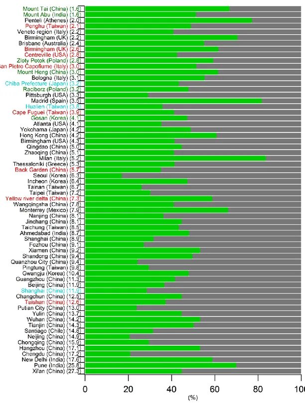
Figure A1 synthesizes the locations of the studies discussed in this section. Detailed references about these results are given in Tables A2 and A3 in the SM. It is important to note that no data (or very few) are displayed here for Africa, Oceania, Central Asia, Russia, Central and South America. This does not imply that no EC tracer studies have been conducted so far at these

places but rather means that they fall outside the specific criteria of this review (PM2.5 fraction andstudies from 2006 to 2016).

3.1.3.1 Studies in America

Seasonal and regional variations of SOA have been examined thoroughly over the North American continent using the EC-tracer method (Day et al., 2015; Docherty et al., 2008; Dreyfus et al., 2009; Kleindienst et al., 2010; Mancilla et al., 2015; Murillo et al., 2013; Pachon et al., 2010; Polidori et al., 2006; Saffari et al., 2016; Saylor et al., 2006; Seguel A et al., 2009; Sunder Raman et al., 2008; Toro Araya et al., 2014; Vega et al., 2010; Yu et al., 2007). Overall, annual SOC levels ranged from 1.1 to 2.7 µgC m-3, contributing to 27-70% of PM2.5 OC (Figure 2; Table A2). The highest contributions (~63% on average) were obtained for rural locations, while at urban sites contributions were in the range of 30 to 50%. SOC estimates in warm period in the USA obtained from the literature showed that 29-43% (1.0-1.8 µgC m-3) of PM2.5 OC was secondary, with the highest contribution (43%, 1.2 µgC m-3_{) at a rural location (Centreville)} (Figure 3, Table A3).

Few examples of SOC estimations are also available in Central and South America (Mancilla et al., 2015; Murillo et al., 2013; Seguel A et al., 2009; Toro Araya et al., 2014; Vega et al., 2010) (Figure 2). The annual average SOC contribution was approximately 57% and reached up to 87% of PM2.5 OC in Mexico (Mancilla et al., 2015) (Figure 2, Table A2). Some other previous studies showed lower SOA contributions (Martinez et al., 2012; Stone et al., 2008), though the estimations were not carried out using the same approach. In Santiago, Chile, no significant differences have been observed between the annual and spring-summer SOC contributions (annual: 29±6% and spring-summer: 31±6%) (Toro Araya et al., 2014). These