Development of an analytical method usefull for the quantification of L-Glu & GlutaMAX during fermentation

(1)

(2)

(3)

Objectives

The objectives of this work are to establish time and cost-efficient methods for the quantification of L-Glutamine and GlutamaxTM in different mediums containing serums. These methods have to be easy to perform and based on a purpose of daily basis analysis of mammalian cells cultures.

Methods | Experien ces | Resu lts

Two methods will be developed in parallel and will allow the monitoring of L-Glutamine and GlutamaxTM during bioprocesses. It is really crucial to quantify the amount of L-Glutamine or GlutamaxTM which gives information about cells viability and metabolism.

Methods that have been developed allow the quantification of L-Glutamine and GlutamaxTM in different media with an iscocratic separation on a RP-HPLC system using a C18 column. The accuracy of both methods is less than +/-10% as well as the reproducibility that is less than 5%. The methods developed are based on a pre-column reaction of derivatization that is controlled automatically by the auto sampler. One of the main parts of these methods development was the optimization of the reaction parameter in order to assure a complete reaction.

A precise SOP for each method will also be developed that will allow people to use these method on daily purpose analysis.

Development of an analytical method useful for

the quantification of L-Glu & Glutamax

TM

during

fermentation

Graduate

Mayor Mathieu

Bachelor’s Thesis

| 2 0 1 3 |

Degree course Life Technologies Field of application Analytical Chemistry Supervising professor Dr. Franka Kalman franka.kalman@hevs.ch

Reaction used for the derivatization of the primary amine of L-Glu and Glutamaxtm.

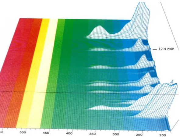
One example of the absorbance spectrum of the media SFM4CHO with the serum hyclone SH30548 using GlutamaxTM as substrate. The peak of GlutamaxTM comes out at 12.4 min

(4)

Table of contents

0. Abbreviations 2

1. Introduction 3

2. Aim and methods requirements 3

3. Theoritical part 4

3.1 Litterature used and strategy 4

4. Experimental part 6

4.1 Materials 6

4.2 Reagants and safety 6

4.3 Sample preparation 7

4.3.1 Method 1 7

4.3.2 Method 2 7

4.4 HPLC systems 8

4.4.1 Isocratic 8

4.4.1.1 Method 1.1 for L-Glutamine 9

4.4.1.2 Method 1.2 for GlutamaxTM 9

4.4.1.3 Method 2.1 for L-Glutamine 10

4.4.1.4 Method 2.2 for GlutamaxTM 10

4.4.2 Gradient 11

4.4.2.1 Method 3.1 11

4.4.2.2 Method 3.2 12

5. Results and discussion 13

5.1 Method development 13

5.1.1 Determination of the sampling method 13

5.1.2 Optimization of the OPA reaction 14

5.1.3 Determination of the wavelength UV detector 17 5.1.4 Determination of the best separation method 20 5.1.5 Determination of the experimental HEPT Curve 29

5.2 Methods requirements 32

5.2.1 Specificity 32

5.2.2 Range 32

5.2.3 Accuracy 33

5.2.4 Precision 33

5.2.5 LOD of the method 34

5.2.6 Linearity 34

5.3 Comparison between kinetics obtained from two different HPLC. 35

5.3.1 SFM4CHO media with L-Glu 35

5.3.2 Sigma media with GlutamaxTM 37

5.4 Others kinetics 39 6. Conclusion 40 7. Prospects 40 8. Acknowledgments 40 9. Literature 41 10. Appendix 42 10.1 Excel tables 42 10.2 Formulas 53

10.3 SOP for method 1.1 55

(5)

0. Abbreviations

HPLC: High performance liquid chromatography LC: Liquid chromatography

HEPT: Theoretical plate height

HPLC-RP: High performance liquid chromatography on reverse phase SOP: Standard operation procedure

L-Glu: L-Glutamine ACN: Acetonitrile MeOH: Methanol

LIF: Laser induced fluorescence DAD: Diode array detector UV: Ultraviolet OPA: ortho-phtalaldehyde 2-MCE: 2-mercaptoethanol λ

: wavelenght [nm]

µ: Flowrate [ml/min]

dp: particles diameter [µm]

w: peak width [min]

Rt: retention time [min]

Lcol: column length [cm]

Rs: resolution

H: Theoretical plate height [cm]

N: Number of theoretical plates

Vinj: injection volume [µl]

(6)

1. Introduction

L-glutamine is an essential component in cell culture media, being used as a source for the energy production of the cell. It also used for the synthesis of proteins and nucleic acids necessary for the cells growth. However, the L-Glutamine is temperature sensitive and thus degrades spontaneously at 37 °C which is the normal temperature of mammalian cells cultures. The degradation of L-Glutamine does not only result in a loss of energy source but also generates ammonia as by-product. The accumulation of ammonia can be toxic for the cells and can affect the glycosylation and cell viability. This drives to a lower protein production for the cells and can also change the glycosylation pattern.

As an alternative to L-Glutamine, a dipeptide had been developed that is more stable than the simple amino-acid in the same conditions. This molecule is called GlutamaxTM and corresponds to the following amino acids sequence: L-Alanyl-L-Glutamine. As mentioned, the considerable advantage of this molecule is its extreme stability in the mammalian cells culture conditions due to its L-glutamine stabilized form. It then prevents the break-down of L-glutamine and thus the formation of ammonia.

Anyways, for each substrate that is chosen, it is really crucial to monitor the amount of L-Glutamine or GlutamaxTM which give information about cells viability and metabolism. In order to quantify the ammonia and the L-glutamine, enzymatic kits or automatic devices are often used. However, these kits and automatic devices are really expensive in themselves and also in their maintenances. In contrast to L-Glu, methods to specifically detect the dipeptides of GlutamaxTM solutions have not been described so far.

2. Aim and method requirements

The objectives of this work are to establish time and cost efficient methods for the quantification of L-glutamine and GlutamaxTM. This method has to be easy to perform and based on a purpose of daily basis analysis of the mammalian cells cultures. The methods also have to be according to the method requirements needed from the biotechnical department. The requirements are described in the following points:

 Specificity: the methods have to be specific for L-Glutamine and GlutamaxTM. Furthermore, it has to be compatible with different medias e.g. serum free and serum containing media.

 Range: the measuring range should lie between 0.1 and 8 mM (0.015 – 1.2 mg/ml for L-glu and 0.0217 – 1,7 mg/ml for glutamax)

 Limit of quantification : limit of quantification should be at least 0.1 mM for each subtracts or lower

 Accuracy: an accuracy (recovery) of +/- 10% is acceptable

 Precision : a precision of +/- 5% (repeatability) is acceptable

 Robustness: the method should run in an easy to perform manner in daily routine circumstances. Easy to perform system suitability testing parameters shall be chosen.

(7)

 Linearity: chose the calibration curve to cover the above mentioned range accordingly and based on practical considerations.

3. Theoretical part

In this section, the main keys of methods choices and methods developments will be given. The methods have to be specific to different medium which are presented in the following table:

Table 1: All different mediums containing serums

Metabolite

Medias with serum

L-Glu Glutamaxtm

SFM4CHO (Hyclone SH30548) × ×

CDCHO ×

DMEM/Ham'F12 (Sigma D6421) with 10% FCS × ×

DMEM/Ham'F12 (Gibico 10743011) with 10% FCS ×

As seen below, the analytical method that will be chosen has to be compatible for each media containing each serum presented in the table 1. Each of the media and serum contain a lot of different molecules that can be really big (like for example some DNA residues or some enzymatic molecules). For this reason, the matrix effect has to be study carefully.

3.1. Literature and strategy

Before searching any publications or literature about this area of research, it is always good to think a little bit by him-self. The main analytical instruments which are often present in laboratories are the LC systems. It is therefore a good idea to try to develop methods on it. The second thing is to think about the separation itself. Once again, one of the most popular analytical methods because of its cost and viability is the HPLC-RP. But how it is possible to separate such a little and relatively polar molecule on a system that retains molecule due to non-polar interaction with physiological pH. The solution that comes rapidly to mind is to use a derivatizing agent that can be able to increase the retention on the reversed phase column of the L-Glutamine or GlutamaxTM. Therefore, L-Glutamine and GlutamaxTM can be detected using a simple RP-HPLC system.

It also appears relatively rapidly that the molecule of OPA is widely used for this purpose. Several publications mentioned the utilization of this reagent for the derivatization of molecules containing primary amines, which is the case of the two molecules of interest. The point of departure was the publication of Jens Olaf Krömer and Michel Fritz (2004) that published about the “In vivo quantification of intracellular amino-acids and intermediates of methionine pathways in Corynebacterium glutamicum”. They described a reaction of derivatization using OPA and under certain conditions and at physiological pH and detected with UV at 338 nm.

(8)

Then, it is needed to find an adequate column for the separation. As the pH is relatively high, the choice of the column was actually specific. Indeed, at theses pH, most of the rp-columns existing will be affected by this parameter and will result in a considerable deterioration of the column. The next step will be the optimization of the derivatization parameters and conditions. In order to reduce the error relative to this reaction, the 1100 auto sampler of Agilent will be used and will also be a non-negligible part of the method development. Once it is working and the molecules of interest detected using an UV-detector, the matrix effect of all media containing serum will have to be studied in order to make an analytical method specific for all mediums. It requires a working handle sampling and also a proper dilution that avoid all matrix effect.

(9)

4. Experimental part 4.1 Materials

HPLC: Series 1100 Agilent from the laboratory f103

 UV detector : G1315A, Serial : DE91606692

 Auto sampler : G1313A, Serial : DE91609213

HPLC: Series 1100 Agilent from the biotechnical department

 UV detector : G1315A

 Auto sampler : G1313A pH Meter: Metrohm 654 pH-Meter

Filters 3kDA: Nanostep 3K Omega, Life Science Micropipettes: from Biohit

All glassware from the laboratory f103 Centrifuge: Hettich, Mikro 200

HPLC Vials of 2 mL

Analytical balance: Metler Toledo, laboratory f103.

Filters 0.45 um: Exapuretm, Syringe Filters PTFE, 0.45µm, 24 mm PTFE membrane

HPLC Column: C18 gravity, Macherey-Nagel, 4,6mm x 150 mm, 3 µm, serial N°: N8090623

4.2 Reagants and safety

Table 2 : Reagents, provenance and safety Compound name Formula Quality

[%]

Origin n° number catalogue

n° CAS Safety Notice

Acetonitrile C2H2N 99.9 Lab-Scan C73C11X 75-05-8 Xn, F -

OPA C8H6O2 99 Sigma P0657

643-79-8

Corrosive, T -

MeOH CH4O 99.9 Lab-Scan C17C11X 67-56-1 T, F -

L-Glutamine C5H10N2O3 99 Sigma G3126 56-85-9 - -

MQ Water H2O - - - -

Glutamaxtm C8H15N3O4 - Invitrogen A12860 - - 200 mM

solution

2-MCE C2H6OS >98 Flukka 63700 B3,D1A,D2B -

Sodium dihydrogen phosphate NaH2PO4.H2O Acros Organics A0331028 10049-21-5 - -

Bicine C6H13NO4 99 Sigma B3876

150-25-4

(10)

4.3 Sample preparation

The preparation of samples and the sampling itself has to be performed well in order to get acceptable results. Two different methods of preparation and storage of samples are presented here. Both of them are acceptable and will be discussed further. Note here that both preparation of sample containing L-Glutamine or Glutamaxtm are the same so there is no consideration about this. The both methods will be discussed later, they are not fundamentally different but they belong to contrasting strategies. Note that all the results that will be presented here result from the method 1 of sampling.

4.3.1 Method 1

Aliquot periodically 1 mL from the culture of mammalian cells, filter it on a 0.45 µm filter (see section 4.1). Store it in the freezer for further analyses. If you use it directly, take 200 µl of the sample and filter it on a 3kDa filters (see section 4.1). In order to do it, run 10 min at 15000 rpm in a centrifuge. Once this is done, add 20 µl of H2O and run another 10 min with the centrifuge. Once it is done, sample 200 µl for further dilutions and analyzes. Again, if the samples are not used directly, store them in the freezer.

4.3.2 Method 2

Aliquot periodically 1 mL from the culture of mammalian cells, filter it on a 0.45 µm filter (see section 4.1). Store it in the freezer for further analyses. If you use it directly, use immediately 200 µl for further analyses. Again, if the samples are not used directly, store them in the freezer.

(11)

4.4 HPLC-RP systems

In this part, the main ideas about the systems that have been developed will be given but only about the separation (not the reaction of derivatization) that (both) will be discussed later.

4.4.1 Isocratic

This is basically the best way to have an efficient separation and has the most chance to work for all mediums assuming that the separation (resolution) will be better. Before going any deeper with the description of the method, the following figure explains the strategy that has been used for all isocratic separation that will be presented:

Figure 2: Strategy of the method development with isocratic separation

Once we can see on the figure 2, for the isocratic methods, there is five different parts. They correspond to the following:

1) Isocratic part for the separation of the molecules of interest

2) Augmentation of the percentage of organic solvent in order to empty the column 3) Augmentation of the percentage of organic solvent in order to empty the column 4) Stabilization of the column for the next injection

5) Stabilization of the column for the next injection

Another important thing to notice before go any further is that, two different methods have been developed in parallel for the L-Glutamine and GlutamaxTM. As GlutamaxTM is the most non-polar molecule of interest, once can assume a longer retention time into the rp-column. That’s why the percentage of organic solvent has to be increased in the case of GlutamaxTM. All other parameters remain the same for each method but -by worries of comprehensibility- the details of all methods will still be given.

(12)

4.4.1.1 Method 1.1 for l-Glutamine

Column: C18 gravity, Macherey-Nagel, 4,6mm x 150 mm, 3 µm, serial N°: N8090623 HPLC system: Series 1100 Agilent, laboratory f103

 Auto sampler : G1313A, Serial : DE91609213 Wavelength UV detector: 338,4 [nm]

Temperature: 25°C

Eluents: ACN and NaH2PO4 (40mM, pH = 7,8)

Table 3: Eluent composition for method 1.1

Time [min] %ACN %Buffer Flow rate [ml/mn] max. pressure [bar]

13 14 86 0.8 300

15 60 40 0.8 300

17 60 40 0.8 300

19 14 86 0.8 300

Stop time: 21 min

4.4.1.2 Method 1.2 for GlutamaxTM

Column: C18 gravity, Macherey-Nagel, 4,6mm x 150 mm, 3 µm, serial N° : N8090623 HPLC system: Series 1100 Agilent, laboratory f103

Wavelength UV detector: 338,4 [nm] Temperature: 25°C

Table 4: Eluent composition for the method 1.2

Time [min] %ACN %Buffer Flow rate [ml/mn] max. pressure [bar]

11 19 81 0.8 300

13 60 40 0.8 300

16 60 40 0.8 300

18 19 81 0.8 300

(13)

4.4.1.3 Method 2.1 for L-Glutamine

 Auto sampler : G1313A, Serial : DE91609213 Wavelength UV detector: 338,4 [nm]

Temperature: 25°C

Eluents: MeOH and NaH2PO4 (40mM, pH = 7,8)

Table 5: Eluent composition for method 2.1

Time [min] %MeOH %Buffer Flow rate

[ml/mn] max. pressure [bar] 13 14 86 0.8 300 15 60 40 0.8 300 17 60 40 0.8 300 19 14 86 0.8 300

Stop time: 21 min

4.4.1.4. Method 2.2 for GlutamaxTM

Eluents: MeOH and NaH2PO4 (40mM, pH = 7,8)

Time [min] %MeOH %Buffer Flow rate

[ml/mn] max. pressure [bar] 11 19 81 0.8 300 13 60 40 0.8 300 16 60 40 0.8 300 18 14 81 0.8 300

(14)

4.4.2 Gradient

For the development of a separation using a gradient of organic solvent, the separation will be harder to proceed but the peaks will have a greater height and that will result in a better limit of detection. The method in itself will be faster and that is a really powerful economic argument. As the matrix effect is relatively complicated to handle, only the working methods will be presented here.

4.4.2.1 Method 3.1 for L-Glutamine

Eluents: ACN and NaH2PO4 (40mM, pH = 7,8) Table 7: Eluent composition for the method 3.1

Time [min] %ACN %Buffer Flowrate [ml/mn] max. pressure [bar]

8 50 50 0.8 300

10 50 50 0.8 300

12 15 85 0.8 300

14 15 85 0.8 300

Starting eluent composing: 15% ACN and 85% Buffer Stop time: 14 min

In order to have a better understanding of the evolution of the eluent during time, the following figure will help to visualize it:

(15)

4.4.2.2 Method 3.2 for L-Glu



Time [min] %ACN %Buffer Flowrate [ml/mn] max. pressure [bar]

2 15 85 0.8 300

9 60 40 0.8 300

11 60 40 0.8 300

13 15 85 0.8 300

Starting eluent composing: 15% ACN and 85% Buffer Stop time: 14min

In order to have a better understanding of the evolution of the eluent during time, the following figure will help to visualize it:

(16)

5. Results and discussion

This is the main part of the report, the choice of methods and the method development will be covered here. By worries of comprehensibility, all the steps will be described here in details, but all the specifications about the analytical method itself will only be given in the SOP in appendix.

5.1 Method development

All the methods about the sampling and also about the analytical methods will be covered and discussed here. Once will be able at the end to clearly understand why and which methods are retained in the SOP.

5.1.1 Determination of the sampling method

For the preparation of the sample, it is two different methods described in section 4.3. The only difference between the both methods is the filtration on the 3 kDa filter (see section 4.1) and the dilution after using the centrifuge. As it has been already mentioned earlier, serums as well as samples or medium can contain really big molecules. The main problem with big molecules is that the pre-column used can be relatively quickly blocked. It is the only problem. As the following figure will express, there is no loss in the response of the molecule of interest but only a loss of molecule that cannot go through the pre column. Another interesting thing to explain is the utilization of 20 µl of H2O MQ that will assure the passage of all the molecules of interest. Indeed, it is possible that after the first centrifugation, some of the molecules can be stuck into bigger one. That’s why the 20 µl of H2O are used.

Figure 5: Comparison between the two samples preparation for the SFM4CHO (Gibico 10743011) medium containing L-Glutamine. In red: without filtration on 3kDA filter. In Blue: with filtration on 3kDA.

On the figure 5, once can see no difference in the response of the molecule of interest (~11.8 min). Therefore, the assumption that the big molecules filtered on 3 kDA cannot go through the pre column should be truthful. It is interesting to discuss the two different way of sampling once this assumption is issued.

(17)

In the case of method 1 of sampling, the pre column is saved but takes more time for the preparation. On the other hand, method 2 is faster but affects the pre column. At this point, it is interesting to have a little guess:

The price of a pre column is about 100 CHF, and can handle up to twelve injections. So for the method 2, the price of 12 injections is then 100 CHF. It is possible to compare this price to the cost of method 1 for the same amount of injections. As it has been noted, the time needed for the sample preparation is 20 min of centrifuge plus about 7 min for the preparation. Assuming that an operator that can run this method is paid about 60 CHF per hour and the cost of one 3kDA filter is about 5 CHF, it is possible to calculate the price for twelve injections as well. As is it trivial, the calculation will not be given here but only the result: 87 CHF. It appears clearly that the method 1 is cheaper and that is the main argument to choose this method of sampling for the SOP. More details about this method of sampling are given in the SOP in appendix.

5.1.2 Optimization of the OPA reaction

Before go any deeper in the method development of the analytical method itself, it is necessary to discuss the optimization of the reaction of derivatization. In order to optimize the reaction that was mentioned by Jens Olaf Krömer and Michel Fritz (2004) in their publication: “In vivo quantification of intracellular amino-acids and intermediates of methionine pathways in

Corynebacterium glutamicum”, a fluorescence lector had been used. All different conditions are

presented in the following table (on the next page) and also the corresponding figure to the data received.

(18)

Table 9: optimization parameters for the OPA reaction Bicine + 2ME 5% [ul] Glu_1 mg/ml [ul] Bicine 0.5 M [ul] OPA 1,04 mg/0.2 ml [ul] H2O [ul] Somme [ul] Scale down [ul]

I.1

4 3 6 6 20 39 19.5 Bicine + 2ME 5% [ul] Glu_1 mg/ml [ul] Bicine 1 M [ul] OPA 1,04 mg/0.2 ml [ul] H2O [ul] Somme [ul] Scale down [ul]

I.2

4 3 6 6 20 39 19.5 Bicine + 2ME 5% [ul] Glu_1 mg/ml [ul] Bicine 0.1 M [ul] OPA 1,04 mg/0.2 ml [ul] H2O [ul] Somme [ul] Scale down [ul]

I.3

4 3 6 6 20 39 19.5 Bicine + 2ME 5% [ul] Glu_1 mg/ml [ul] Bicine 0.5 M [ul] OPA 1,04 mg/0.2 ml [ul] H2O [ul] Somme [ul] Scale down [ul]

I.4

6 3 6 6 20 41 20.5 Bicine + 2ME 0.5% [ul] Glu_1 mg/ml [ul] Bicine 0.5 M [ul] OPA 1,04 mg/0.2 ml [ul] H2O [ul] Somme [ul] Scale down [ul]

I.5

6 6 6 6 20 44 22

I.5'

4 6 6 6 20 42 21

I.6

4 6 6 6 20 42 21

I.7

6 6 6 6 40 64 32

I.8

4 6 6 6 40 62 31 Bicine + 2ME 0.5% [ul] Glu_1 mg/ml [ul] Bicine 0.5 M [ul] OPA 1,04 mg/0.2 ml [ul] H2O [ul] Somme [ul] Scale down [ul]

final 1

4 6 6 6 40 62 31 Bicine + 2ME 0.5% [ul] Glu_0,1 mg/ml [ul] Bicine 0.5 M [ul] OPA 1,04 mg/0.2 ml [ul] H2O [ul] Somme [ul] Scale down [ul]

final 2

4 6 6 6 40 62 31 Bicine + 2ME 0.5% [ul] Glu_1 mg/ml [ul] Bicine 0.5 M [ul] OPA 1,04 mg/0.2ml [ul] H2O [ul] Somme [ul] Scale down [ul]

final 3

4 6 6 6 40 62 31 Bicine + 2ME 0.5% [ul] Glu_1 mg/ml [ul] Bicine 0.5 M [ul] OPA 0.5 mg/0.2ml [ul] H2O [ul] Somme [ul] Scale down [ul]

final 4

4 6 6 6 40 62 31 Bicine + 2ME 0.5% [ul] Glu_1 mg/ml [ul] Bicine 0.5 M [ul] OPA 0.1 mg/0.2ml [ul] H2O [ul] Somme [ul] Scale down [ul]

final 5

4 6 6 6 40 62 31 Bicine + 2ME 0.5% [ul] Glu_1 mg/ml [ul] Bicine 0.5 M [ul] OPA 2,5 mg/0.2ml [ul] H2O [ul] Somme [ul] Scale down [ul]

final 6

4 6 6 6 40 62 31

(19)

As only the results from the final systems will be plotted here, it is interesting to comment this table 9 a little bit. As it can be seen, the experiments I.1, I.2 and I.3 show the effect of different concentration of bicine in the reaction. It appears that a concentration of 0.5 M drives to a better amount of fluorescence. Then, I.4 shows that the concentration of the 2-mercaptoethanol has to be lower than it is in I.1, I.2 and I.3. So, I.5, I.5’, I.6, I.7, I.8 are only different concentration of

2-mercaptoethanol using different dilution in order to optimize this parameter.

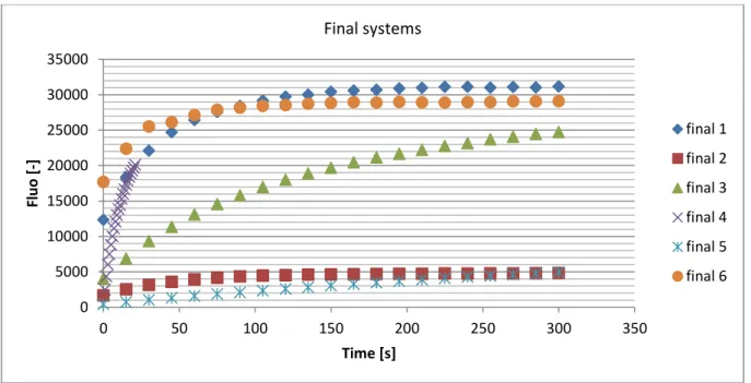
The following figure will express the final systems that have been retained due to

experiments ran before (I.1 to I.8), the system with the more amount of fluorescence will be retained for the derivatization conditions.

Figure 6: Plot of final systems conditions for the derivatization

The conditions that have been retained are the system final 6. It is visible on the figure 6 that the system final 6 has one of the most amounts of fluorescence. It is also visible that the kinetics of this reaction follows a first order and is really fast. The half time is almost reach during the time that the reagent is put in the box and enters the fluorescence lector. This shows how specific and fast the reaction is. Note that the system called final 4 encountered some troubles that drive to this relatively strange results. Note also that the final 6 parameters drive to a dilution of 10,33 of the sample that will be really important for the further analyzes.

0 5000 10000 15000 20000 25000 30000 35000 0 50 100 150 200 250 300 350 Fl u o [ -] Time [s] Final systems final 1 final 2 final 3 final 4 final 5 final 6

(20)

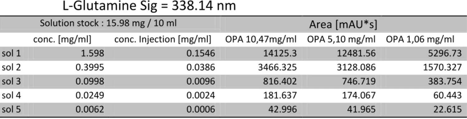
The following table will confirm the data obtained in the table 9. It is actually different HPLC runs with different concentration of OPA used that correspond to systems finals presented in table 9:

L-Glutamine Sig = 338.14 nm

Solution stock : 15.98 mg / 10 ml

_{Area [mAU*s]}

conc. [mg/ml] conc. Injection [mg/ml] OPA 10,47mg/ml OPA 5,10 mg/ml OPA 1,06 mg/ml

sol 1 1.598 0.1546 14125.3 12481.56 5296.73

sol 2 0.3995 0.0386 3466.325 3128.086 1570.327

sol 3 0.0998 0.0096 816.402 746.719 383.754

sol 4 0.0249 0.0024 181.637 174.067 60.443

sol 5 0.0062 0.0006 42.996 41.965 22.615

5.1.3 Determination of the wavelength UV detector

In order to define a wavelength for the UV detection, a 3D spectrum of all the absorbance from a sample of SFM4CHO is taken. First of all, this is done in order to confirm that the wavelength used by Jens Olaf Krömer and Michel Fritz (2004) in their publication: “In vivo quantification of intracellular amino-acids and intermediates of methionine pathways in Corynebacterium

glutamicum” is valuable. It is also done to check the relative purity of the peak, as it was possible to

use a DAD detector. The strategy is relatively simple: the 3D spectrum of all the absorbance from 200 to 600 nm will show where the impurity can hide at the elution time of the molecule of interest.

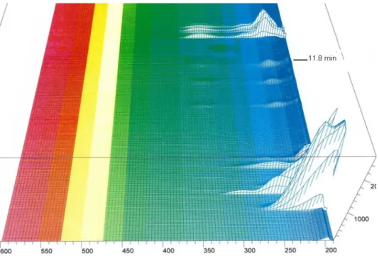
Figure 7: 3D spectrum of 200 to 600 nm of the absorbance for SFM4CHO (Hyclone SH30548) with method 1.1

(21)

It is possible to see that the wavelength of 338 is relatively specific and is a good wavelength in order to detect the L-Glutamine (it comes out at about 11.8, figure 8). In the case of the method 1.1 and the L-glutamine, no impurities are detected. It is possible to fix the wavelength at 338 and will empty the chromatogram from all the peaks that come out from 200 to 300 nm.

For the method 1.2, it is almost the same results as it is the same medium and serum that was analyzed. The following figures represent the 3D spectrum of same wavelengths that had been used for figure 7 and 8.

(22)

The molecule of interest is detected at about 12.4 min, as for the figure 7 and 8, it can be seen that the choice of a wavelength of 338 nm is a relatively good choice. And that, for the same reasons that was stated before, in an optic of refining the chromatograms.

(23)

5.1.4 Determination of the best separation method

As seen above, several methods had been developed and the next step is to define which of these methods of separation are the most appropriate for the system. All the methods will be described in more details with some chromatogram to illustrate them. Then, the method chosen will be discussed with more precision.

The first two methods that are going to be discussed are the method 2.1 and the method 2.2. As seen above, the only difference with the method 1.1 and 1.2 are the organic solvent that is used. For the case of 1.1 and 1.2, acetonitrile has been used and for the others, it was methanol. Both methods provide a good separation with decent resolutions. The main problem that was

encountered was the methanol potential to change significantly the viscosity of the eluent. And this drives to a really strong difference on the pressure during the phase 2, 3 and 4 of the figure 2. As we can see on table 3, 4, 5, 6, 7, 8, the max pressure is 300 Bar. For this reason, and as many

experimental problems were encountered about the max pressure, the method 2.1 and 2.2 are not retained. For example, during the phase 3 of figure 2, for a flow rate of 0.8 ml/min, the pressure reached 280 Bar. Hence, these two methods were not retained in the optic of plotting an HEPT experimental curve. Indeed, the assumption that the pressure of higher flow rate with the same conditions would exceed 300 Bar.

In comparison to the methods 2.1 and 2.2, methods 1.1 and 1.2 do not have this problem which is a relatively good point for these methods. It was no differences between the statistics calculated for the both methods but only this problem of viscosity. That’s why the statistics of the methods 2.1 and 2.2 as well as their chromatograms will not be given here as they have no real interests. Therefore, methods 2.1 and 2.2 will be eliminated for this purely practical reason.

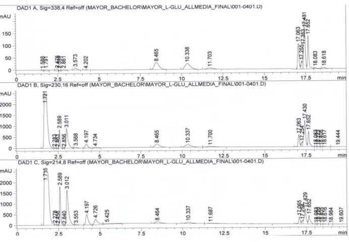
The following figures present the different chromatograms obtained with all medium and serum for the methods 1.1.

(24)

Figure 12: L-Glutamine with CDCHO using method 1.1

(25)

Figure 14: L-Glu tamine with SFM4CHO (Hyclone SH30548) using method 1.1

The retention time and the resolutions for each medium are related in the next table: Table 10: retention time statistics for all media and resolution from method 1.1

L-Glu_method 1.1 Rt [min] Rs DMEM/Ham'F12 (Sigma D6421) 11.847 4.24 CDCHO 11.703 3.57 DMEM/Ham'F12 (Gibico 10743011) 11.85 4.06 SFM4CHO (Hyclone SH30548) 11.826 3.85 Average [min] 11.8065 SD_tR [min] 0.06046693 RSD_tR[%] 0.51214952

From a purely experimental point of view, method 1.1 could be validated for all medium with L-glutamine as subtract. The next point will be the optimization of the flow rate with the calculation of the number of theoretical plates (N) that will result in a plot giving the HEPT curve. It will be treated in the further discussion.

(26)

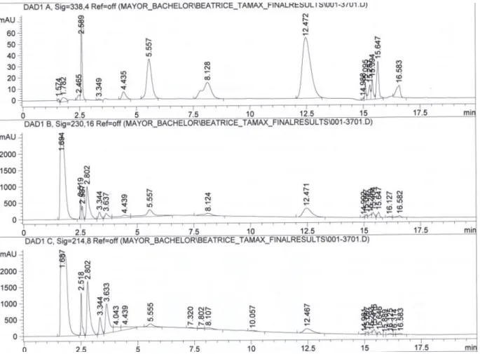
The chromatograms for the methods 1.2 for all medium are also given in the following figures:

(27)

Figure 16: Glutamaxtm with SFM4CHO (Hyclone SH30548) using method 1.2

The statistics about retention times for both medium is presented in the following table. Note that the resolution has not been calculated due to the absence of any peaks near the retention time of the molecule of interest in the UV region.

Table 11: retention time statistics for all medium using method 1.2 Glutamaxtm_method 1.2 tR [min]

DMEM/Ham'F12 (Sigma D6421) 12.503 SFM4CHO (Hyclone SH30548) 12.472

Average 12.4875

SD_tR 0.0155

(28)

The reason why the organic solvent is not higher is because with a FLD detector, it is possible to detect an impurity as we will see on the next figure:

Figure 17: FLD detection (Ex=230, Em=450) of Glutamaxtm with SFM4CHO (Hyclone SH30548) using method 1.2

The resolution calculated between these two peaks is 2.6, that is acceptable. It would be also accepted to work with a higher amount of acetonitrile as the impurity peak represents only 0.6% of the peak area of the molecule of interest. By worries of having some changes in the mediums or in the serum used in the future, a safe separation was preferred.

At this point, it is a good to make a recapitulation of what it has been seen until now. We have discussed the difference between the method 1.1 and 1.2 versus the method 2.1 and 2.2. It has appeared that the method 2.1 and 2.2 have some practical problems that drive to the abandon of these two methods even if they present the same quality of separation that 1.1 and 1.2 do have. In order to push the discussion a little bit forward, it is a good time to discuss the two last methods involving a gradient separation.

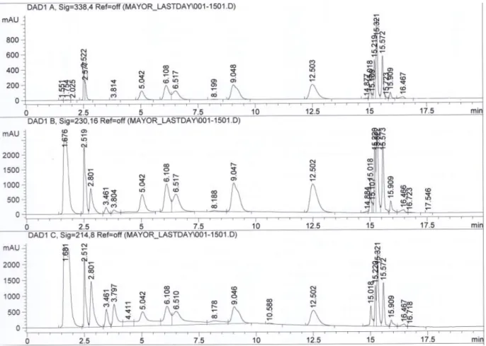
The method 3.1 as well as the method 3.2 involve a gradient separation which has the effect of refining the peaks and will result in a better detection limit. The problem of this kind of separation is the lower robustness. Assuming the method should be robust and able to adapt on different HPLC, an isocratic separation is preferred. Note that is not the only reason, indeed some change in medium and serum can happen and the method will not be able to adapt. However, this is still interesting and the results about the two methods developed will still be given and discussed briefly. The following figures will present some results using these methods for L-glutamine only.

(29)

Figure 18: L-Glutamine with SFM4CHO (Hyclone SH30548) using method 3.1

(30)

Figure 20: L-Glutamine with CDCHO using method 3.1

(31)

The statistics about the retention time and the resolutions for the method 3.1 are presented in the following table:

Table 12: retention time statistics for all media and resolution from method 3.1

L-Glu_method 3.1 Rt Rs DMEM/Ham'F12 (Sigma D6421) 5.79 2.36 SFM4CHO (Hyclone SH30548) 5.78 1.49 CDCHO 5.722 1.51 DMEM/Ham'F12 (Gibico 10743011) 5.792 2.32 Average 5.771 SD_tR 0.03308575 RSD_tR[%] 0.57331047

As it is possible to see on the table 11, the RSD relative to the retention time is only 0.5%. On the others hand, the resolution calculated for the method 3.1 is still usable but as it has been already said above, any little change in mediums or serums can fast drive into some problems of the

separation of the molecules that the method want to separate. However, this method is still

performable in an economic optic. But once again, the accent had been put on the separation itself and not on pure statistics and economic pressure.

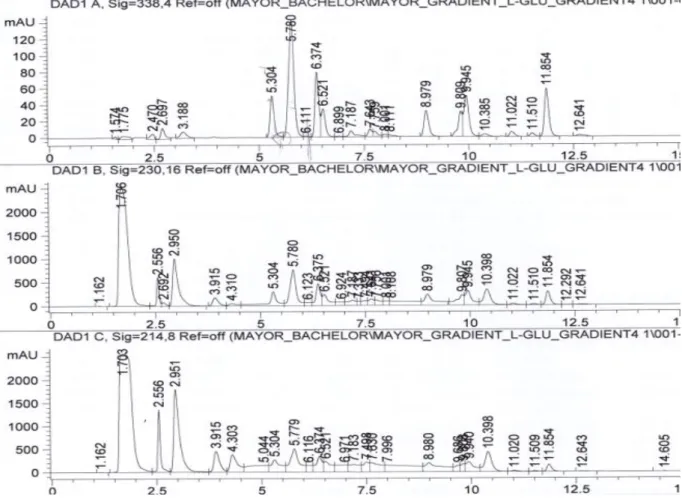
For the method 3.2, the approach is relatively different. As we can see on the figure 3, it starts with an isocratic mode for 2 min before it goes to a gradient mode. As it is less interesting for the report as one medium does not separate decently, only one example of chromatogram will be given here.

(32)

Once again, all the methods that are presented here are viable. All the statistics are decent and the only argument that will force to make a choice is the quality of the separation. As it had been already said, the method 2.1 and 2.2 are not viable from an experimental point of view. And also from the fact that generally it is not used to work with a higher pressure than 300 Bars. For the method 3.1 and 3.2, their elegance is not enough to fill in the problem that could be encountered with any changes in the matrix. So, the most safe and reproducible choice to make is to retain the method 1.1 and 1.2.

Note also that because of an experimental consideration, the gradient could not go higher than 60% for the simple reason that the buffer could precipitate a bit when it goes more than 60% of organic solvent.

5.1.5 Determination of the experimental HEPT Curve

The final step in order to optimize methods 1.1 and 1.2 that had been developed is to plot the HEPT curve. This curve expresses the theoretical plate height (H) in function of the flow rate and represents the Van Deemter plot that is the sum of three different functions. In order to do this, it is necessary to calculate the number of theoretical plates (N). All is presented in the following figures:

Figure 23: Theoretical plates for method 1.1

y = 0.0000993x - 0.0021130 0.6 ml/mn y = 0.0000747x - 0.0010228 0.7 ml/mn y = 0.0000747x - 0.0007444 0.8 ml/mn y = 0.000080x - 0.000493 0.9 ml/mn y = 0.0000816x - 0.0003199 1 ml/mn 0 0,002 0,004 0,006 0,008 0,01 0,012 0,014 0,016 0 50 100 150 200 250

w

^2

/16

t

R

^2

Theoretical plates 0.6 ml/mn_L-glu 0.7 ml/mn_L-glu 0.8 ml/mn_L-glu 0.9 ml/mn_L-glu 1 ml/mn_L-glu

(33)

Table 13: Number of theoretical plates for method 1.1 Flow rate [ml/min] N H [cm]

0.6 10070 0.0014895

0.7 13386 0.0011205

0.8 13210 0.0011205

0.9 12500 0.0012

1 11627 0.00129

Once we know the number of theoretical plates (N), it is possible to plot the HEPT curve and the following figure will express it for the method 1.1.

Figure 24: Experimental HEPT Curve for L-Glu with method 1.1

The same calculation has not been done for the method 1.2 because it was not possible to calculate the number of theoretical plates in the same way it was done for the method 1.1. Indeed, as it can be seen on figure 11 and 12, there is no peaks available near the peak of GlutamaxTM. But the theoretical plates can be calculated for the peak only.

Table 14: Number of theoretical plates for method 1.2

Flowrate [ml/mn] N H [cm] 0.6 9710 0.001544 0.7 11846 0.001266 0.8 11533 0.001300 0.9 10875 0.001379 1 10454 0.001434 0,001 0,0011 0,0012 0,0013 0,0014 0,0015 0,0016 0,5 0,7 0,9 1,1 H [ cm ] Flowrate [ml/mn]

Experimental HEPT Curve for L-Glu

(34)

Figure 25: Experimental HEPT curve for L-Glu with method 1.1

We can see on figure 21 and 22 that the optimal region of the curve is between 0,7 and 0,8 ml/mn for the method 1.1 and it is 0,7 for the method 1.2. A flow rate of 0.8 ml/min is then fixed for both methods. It is interesting to think about the parameters that can influence the value of H. As is it relative to the peak shape and width, it is assumable that it will depend on the diameter of the column as well as the diameter of the particles in the column. Its length will also influence it and as it has been shown above, the flow rate will also play a role. More generally it depends of the quality of the column. 0,001 0,0011 0,0012 0,0013 0,0014 0,0015 0,0016 0,5 0,7 0,9 1,1 H [ cm ] Flowrate [ml/mn]

Experimental HEPT Curve for Glutamax

experimental HEPT curve for Glutamax

(35)

5.2 Methods requirements

In this section, only the results from the needed requirements are presented.

5.2.1 Specificity

As it has been already said, the methods 1.1 and 1.2 are specific for each medium containing each serum.

5.2.2 Range

The range that was needed to cover is 0.015 – 1.2 mg/ml for L-glutamine and 0.0217 – 1,7mg/ml for the GlutamaxTM. Note that the samples are diluted 34.1 times before the injection. Following figures will show examples of calibrations used for method 1.1 and 1.2:

Figure 26: Calibration cruve for L-Glutamine_Agilent 1100_F103 using area.

Figure 27: Calibration curve for GlutamaxTM_Agilent 1100_F103 using height. y = 103027x - 14,57 R² = 1 0 1000 2000 3000 4000 5000 0 0,01 0,02 0,03 0,04 A re a [ m A U* s] Concentration [mg/ml] Calibration L-Glu_Agilent 1100_F103 Calibration L-Glu_Agilent 1100_F103 Linéaire (Calibration L-Glu_Agilent 1100_F103) y = 2430x + 1,619 R² = 0,9993 0 20 40 60 80 100 0 0,01 0,02 0,03 0,04 H e ig h t [m A U] Concentration [mg/ml]

Calibration glutamax_Agilent 1100_biotech

Série1

(36)

5.2.3 Accuracy

For this part, two solutions of known concentrations had been used in order to calculate the recovery. It is acceptable to have an accuracy of +/- 10%.

Table 15: accuracy for method 1.1

Precision L-Glu (n=3) concentration : 57,11 mg / 100 ml = 0.5711 mg/ml

concentration th. After dilution : 0.01842 mg/ml

Area [mAU*s]

Average

1693.183 1700.424 1688.57971 1690.5477

concentration calculated : 0.01823 mg/ml

% recovery 98.97

Table 16: accuracy for method 1.2

Precision Glutamaxtm (n=3)

solution : 1485 ul / 100 ml. Glutamaxtm (MW = 217.22, Conc. = 200 mM). Concentration th. after dilution : 0.02081 mg/ml

Area [mAU*s]

Average

1359.29967

1356.325 1360.32 1361.254

concentration calculated: 0.02024 mg/ml

% recovery 97.26

The recovery calculated for each method is less than +/- 10%. Note that it will be the value used in the SOP by safety.

5.2.4 Precision

Table 17: repeatability for method 1.1

Rt [min] Height [mAU] Area [mAU*s]

n=1 5.77 1780.067 98.190 n=2 5.88 1797.776 98.528 n=3 5.85 1843.527 98.632 n=4 5.78 1798.979 98.663 n=5 5.66 1774.429 98.744 n=6 5.65 1768.367 98.726 Average 5.77 1793.857 98.580 SD 0.106 27.299 0.206 RSD 1.846 1.521 0.209

(37)

5.2.5 LOD of the methods

Table 18: LOD for the method 1.1

L-glu DAD Sig = 338.14

Solution stock : 15.98 mg / 10 ml

conc. [mg/ml] conc. Injection [mg/ml] mole/litre Area [mAU*s] Height [mAU] solution 1 1.598 0.15465015 0.001058233 14125.3 415.055 solution 2 0.3995 0.038662538 0.000264558 3466.325 115.641 solution 3 0.099875 0.009665634 6.61396E-05 816.402 32.01 solution 4 0.02496875 0.002416409 1.65349E-05 181.637 7.64 solution 5 0.006242188 0.000604102 4.13372E-06 42.996 1.758 solution 6 0.003121094 0.000302051 2.06686E-06 19.842 0.8389 solution 7 0.001560547 0.000151026 1.03343E-06 9.546 0.3856

solution 8 0.000780273 7.55128E-05 5.16715E-07 4.264 0.196

LOD : 0.00052 mM

Table 19: LOD for the method 1.2

Glutamax

TM

DAD Sig = 338.14

Solution stock : 3450 ul / 100 ml

conc. [mg/ml] conc. Injection [mg/ml] mole/litre Area [mAU*s] Height [mAU] solution 1 1.498818 0.145051582 0.000667763 9410.545 322.542 solution 2 0.3747045 0.036262896 0.000166941 2456.325 79.654 solution 3 0.093676125 0.009065724 4.17352E-05 559.975 22.401 solution 4 0.023419031 0.002266431 1.04338E-05 130.835 5.658 solution 5 0.005854758 0.000566608 2.60845E-06 30.256 1.335 solution 6 0.002927379 0.000283304 1.30423E-06 17.286 0.623 solution 7 0.001463689 0.000141652 6.52113E-07 7.965 0.245 solution 8 0.000731845 -- -- -- -- LOQ: 0.00065 mM

The limit of detection had to be less or equal to 0.1 mM for both methods. It is reached and is about 200 times lower without using an FLD detector. Note that it is also possible to use an FLD detector that will result in a lower LOD.

5.2.6 Linearity

In order to avoid all problems from the matrix effect, a dilution of 34.1 times is performed. It corresponds to the sum of the dilution of all manipulations. This dilution coefficient corresponds of a dilution of 3.3 times for the samples preparation of the samples and 10.333 times for the reaction of derivatization in the syringe of the injector.

(38)

5.3 Comparison between kinetics obtained from two different HPLC.

In order to illustrate the robustness of the method 1.1 and 1.2, the following section will compare the results from two different experiments run on two different series1100 of agilent.

5.3.1 SFM4CHO media with L-Glu

Figure 28: comparison between two same sample series on two different HPLC systems with method 1.1 (Beatrice is the samples name)

Table 20: numerical values of figure 24

Agilent1100_f103 [mg/ml] Agilent1100_biotech [mg/ml] Bea 0 1.041 1.018 Bea 1 0.929 0.892 Bea 2 0.681 0.642 Bea 3 0.462 0.420 Bea 4 0.263 0.233 Bea 5 0.251 0.209 Bea 6 0.241 0.171 Bea 7 0.243 0.190 Bea 8 0.242 0.181 Bea 9 0.249 0.203 Bea 10 0.260 0.204 Bea 11 0.271 0.223 Bea 12 0.271 0.228 Bea 13 0.269 0.223 Bea 14 0.269 0.233 0 0,2 0,4 0,6 0,8 1 1,2 0 5 10 15 20 co n c. [m g/ m l] t [days]

SFM4CHO (Hyclone SH30548)_Beatrice

SFM4CHO_Beatrice_labof103 SFM4CHO_beatrice_biotech

(39)

As it can be seen, only the concentration of the same samples using two different HPLC is given here. But it is also interesting to compare the responses for more injections of the same solutions. Sadly, no accuracy test had been done for the second HPLC, but it is possible to compare data about the calibration curve used, as the solutions used come from the stock solution.

Table 21: Statistics about method 1.1 using height and Agilent 1100 from laboratory f103

Series 1100 Agilent from laboratory f103

Height [mAU] Average [mAU] SD [mAU] RSD [%] 147.365 144.848 145.616 145.943 1.2899 0.88

30.649 30.446 31.621 30.905 0.6280 2.03

5.7644 5.735 5.622 5.707 0.0751 1.31

0.9682 0.97007 0.96552 0.967 0.0022 0.23

Table 22: Statistics about method 1.1 using area and Agilent 1100 from laboratory f103

Area [mAU*s] Average [mAU*s] SD [mAU*s] RSD [%] 3843.33 3843.73 3849.07 3845.376 3.2047 0.083

754.4 755.03 756.536 755.322 1.0975 0.14

136.8 137.534 134.209 136.181 1.7467 1.28

21.614 21.505 21.15609 21.425 0.2392 1.11

Table 23: Statistics about method 1.1 using height and Agilent 1100 from biotechnical department

Series 1100 Agilent from biotechnical department

Height [mAU] Average [mAU] SD [mAU] RSD [%] 104.45 98.36 97.65 100.153 3.7379 3.73

19.985 21.446 20.54 20.657 0.7374 3.57

3.941 3.915 3.965 3.940 0.0250 0.63

0.783 0.822 0.7956 0.800 0.0199 2.48

Table 24: Statistics about method 1.1 using area and Agilent 1100 from biotechnical department

652.23 651.24 653.545 652.338 1.156 0.17

114.565 112.025 111.254 112.614 1.732 1.53

17.167 17.622 17.264 17.351 0.239 1.38

It appears clearly that for each case, the HPLC used in the laboratory f103 had lower relative standard deviation.

(40)

5.3.2 Sigma media with GlutamaxTM

Figure 29: comparison between two same sample series on two different HPLC systems with method 1.2

Table 25: numerical values of figure 25

Agilent1100_f103 [mg/ml] Agilent1100_biotech [mg/ml] Sigma 0 0.831 0.845 Sigma 1 0.798 0.781 Sigma 2 0.757 0.730 Sigma 3 0.688 0.652 Sigma 4 0.671 0.638 Sigma 5 0.667 0.638 Sigma 6 0.660 0.615 Sigma 7 0.662 0.637 Sigma 8 0.664 0.663

As it can be seen, only the concentration of the same samples using two different HPLC is given here. But it is also interesting to compare the responses for more injections of the same solutions. Sadly, no accuracy test had been done for the second HPLC, but it is possible to compare data about the calibration curve used, as the solutions used come from the stock solution.

0,5 0,55 0,6 0,65 0,7 0,75 0,8 0,85 0,9 0 2 4 6 8 10 co n c. [m g/ m l] t [days] DMEM/Ham'F12 (Sigma D6421) Sigma_labof103 Sigma_biotech

(41)

Table 26: Statistics about method 1.2 using height and Agilent 1100 from laboratory f103

Height [mAU] Average [mAU] SD [mAU] RSD [%]

98.812 88.265 92.56 93.212 5.304 5.69

21.735 21.613 21.965 21.771 0.179 0.82

5.1756 5.245 5.365 5.262 0.096 1.82

1.122 1.185 1.154 1.154 0.032 2.73

Table 27 : Statistics about method 1.2 using area and Agilent 1100 from laboratory f103

Area [mAU*s] Average [mAU*s] SD [mAU*s] RSD [%]

2506.679 2482.855 2456.581 2482.038 25.059 1.01

603.178 598.041 601.256 600.825 2.595 0.43

136.924 136.375 136.623 136.641 0.275 0.20

27.306 30.703 28.569 28.859 1.717 5.95

Table 28: Statistics about method 1.2 using height and Agilent 1100 from biotechnical department

Height [mAU] Average [mAU] SD [mAU] RSD [%]

53.778 55.434 54.254 54.489 0.853 1.56

13.508 14.978 13.965 14.150 0.752 5.32

3.799 3.852 3.758 3.803 0.047 1.24

0.993 0.956 0.985 0.978 0.019 1.99

Table 29: Statistics about method 1.2 using area and Agilent 1100 from biotechnical department

315.364 308.654 309.658 311.225 3.619 1.16

88.068 82.752 85.598 85.473 2.660 3.11

22.049 22.086 22.056 22.064 0.020 0.09

It appears clearly that for each case, the HPLC used in the laboratory f103 had lower relative standard deviation. If these result are compared to the tables 21, 22, 23 and 24, once can see that the errors are more important here. It can be explained by the quality of the molecule used. Indeed, for the case of the method 1.2 and Glutamaxtm no specification about the purity of molecules was given and therefore it was not possible to guarantee that all the dipeptides are L, L. This can drive to this difference in the response error.

(42)

5.4 Others kinetics

The following table will present analyzes of last missing samples:

Figure 30: all others kinetics from different samples

In the case of BR3.6 and BR2.0, relatively strange results are calculated. Indeed, the concentration of t0 found for both experiment are higher than the range imposed in the

requirements. But it is still possible to observe the kinetic of the Glutamaxtm degradation over the time. 0 0,5 1 1,5 2 2,5 3 0 2 4 6 8 10 12 co n c. [m g/ m l] t [days]

All other kinetics of different samples

L-Glu_SFM4CHO (Hyclone SH30548)_Beatrice_Agilent1100_ labof103" Glutamax_SFM4CHO (Hyclone SH30548)_BR3.6_Agilent1100_la bof103 Glutamax_SFM4CHO (Hyclone SH30548)_BR2.0_Agilent1100_la bo103

(43)

6. Conclusion

This study has developed a brand new way in order to quantify the L-Glutamine and the Glutamaxtm in complex matrixes enabling the derivatization pre-injection in the needle of the injector. This method will allow the users to make significant economies because of its cheap and easy to perform manipulations needed. But it will also allow really small error on the reaction of derivatization that would significantly be increased in case of manual manipulation. This was the main key of this study, to accomplish a working method which was

economically viable. Indeed, some methods were already usable for the quantification of L-Glutamine but relatively expensive and not so easy to perform as well as their maintenances. In the case of the dipeptide called Glutamaxtm, it was actually no direct methods allowing the quantification of this molecule. So it is with a great pleasure that the operator presenting his method and thus, despite the fact that it is two different methods and not only one.

In a personal point of view, this work was really enriching for the operator. It has allowed a personal elaboration of the strategy for the separation in an atmosphere of trust. This is a really important key for the development of an ingenious mind that will be required in the industry. But not only: this work also allows the operator to be familiar with all aspects of the technique of LC- system used for the separation which is priceless. It also allows the understanding of one of the main problem of the analytical work in industry that is the sampling.

7. Prospects

There are several points that can be stated in this part. First of all, if the analyzes have to reach a lower limit of detection, it is possible to work with a FLD detector using the following wavelength of excitation and emission: Ex = 230 nm, Em= 450 nm.

A second point that can be mentioned is the dwell time optimization of the HPLC from the biotechnical department. Indeed, it is significant change in the retention time between the two HPLC used. Note that it can also be the system of eluent splitting that can drive to different retention time. However, since the resolution is always more than 1.5 it would only be some kind of optimization. Note that it is not only for this experiment but more generally for all experiments driven on this HPLC.

What can also be noticed here is the possibility to optimize methods 1.1 and 1.2 to make only one method with both of them. Sadly, this was not possible due to the significant difference in the retention time as well as the matrix effect that is really hard to handle.

8. Acknowledgments

I would like to take the opportunity to thank all people from the laboratory f103 with a special motion for Antoine Fornage that never hesitated to share is extreme experience about analytical instruments. I would like to thank him as well for all advices and the solutions he purposed to me. He is one of the main key of the success of this work. Special mention for Pascal Jacquemettaz that was always able to listen and offer practical solutions. He is also the one that motioned the utilization of the rp-column that can handle a relatively basic pH. I would also thank the apprentice Aurélien Ducrey that supported me for about one month and help me to handle some problems encountered.

The last motion is for my professor in the HES-SO Valais, the Prof. Franka Kalman for his extreme kindness and knowledge that allows me to rapidly understand problems. I would like to thank her also so his availability that permitted to lead this project to a useful end.

(44)

9. Literature

[1] User requirement specifications, test method to quantify L-glutamine and Glutamax in culture medium during bioprocess, cell culture laboratory, HES-SO Sion, version 2, January 2013

[2] Jens Olaf Krömer, Michel Fritz, In vivo quantification of intracellular amino-acids and

intermediates of methionine pathways in Corynebacterium glutamicum, analytical biochemistry 340 171-137, 2004

[3] Sonja Hess, Kirk r. Gustafson, Dennis j. Milanowski, Chirality determination of unusual amino-acids using a pre-column derivatization and liquid chromatography-electrospray ionization mass spectrometry, Journal of chromate. A, 1035 211-219, 2004

[4] Sadettin S. Ozturk, Bernhard O. Palsson, Chemical decomposition of Glutamine in Cell culture media: Effect of media type, pH, and serum concentration” Biotechnol. Prog.,6 121-128, 1990 [5] G. L. Tritsch, G. E. Moore, Spontaneous decomposition of glutamine in cell culture media, Experimental cell research, 28 360-364, 1962

[6] t. Stoll, p. Pugeaud, U. von Stockar, A simple HPL technique for accurate monitoring of mammalian cell metabolism, Cytotechnology, 14 123-128, 1994

[7] Jens O. Krömer, Stefanie Dietmair, Shana S. Jacob, Quantification of l-alanyl-L-glutamine in mammalian cell culture broth: evaluation of different detectors, analytical biochemistry, 416 129-131, 2011

[8] Stefanie Dietmair, Nicholas E. timmins, Towarsd quantitative metabolomics of mammalian cells: development of a metabolite extraction protocol, analytical biochemistry, 404 155-164, 2010 [9] The retention Behavious of RP-HPLC column, LC-GC Europe, July 2013

[10] Huang Xionfeng, Xu Qun, Joeffrey Rohrer, Automatic precolumn derivatization for the HPLC determination of aliphatic amines in air, application note, Thermo scientific, 2009

(45)

10. Appendix

10.1 Excel tables

(46)

(47)

 Precision

PRECISION : Agilent 1100_labof102

Précision L-Glu (N=3)

concentration : 57,11 mg / 100 ml = 0.5711 mg/ml

concentration th. après dilutions : 0.01842317 mg/ml

**Area [mAU*s]**

Average

1700.424 1688.57971 1690.5477 1693.18395 concentration calculée : 0.018233331 mg/ml

% recovery 98.97047626

Précision GlutaMAX (N=3)

solution : 1485 ul / 100 ml. Glutamax( MW = 217.22 , Conc. = 200 mM). concentration th. après dilutions : 0.02081114 mg/ml

**Area [mAU*s]**

Average

1356.325 1360.32 1361.254 1359.29967 concentration calculée : 0.02024264 mg/ml

(48)

 SFM4CHO_comparison_l-glu

(49)

(50)

(51)

(52)

(53)

 OPA Reaction optimization

(54)

 L-Glu Flowrate

(55)

(56)

10.2 Formulas

The symbols in the following equations correspond to the description of section 0.

(57)

(58)

1. Principle of separation

Using a RP-HPLC with UV-Vis detector, this method allows quantifying of the L-Glutamine in different medium containing serum used for the culture of mammalian cells. The requirements of the method are presented in the following points:

 Range: the measuring range should lie between 0.1 and 8 mM (0.015 – 1.2 mg/ml)

 Accuracy: an accuracy (recovery) of +/- 10% is acceptable

 Precision : a precision of +/- 5% (repeatability) is acceptable

2. Area of application

The RP-HPLC method is formulated to provide a good separation of the L-Glutamine in complex matrix. The different mediums and serum are presented in the following table:

Table 30: All different mediums containing serums

Metabolite

Medias with serum L-Glu

SFM4CHO (Hyclone SH30548) ×

CDCHO ×

DMEM/Ham'F12 (Sigma D6421) with 10% FCS × DMEM/Ham'F12 (Gibico 10743011) with 10% FCS ×

HES-SO

Analytical procedure for the quantification of L-Glutamine in different medium containing serums using RP-HPLC with UV

detection

SOP

Edition : 1 Domain : CA

(59)

3. Safety and precautions

Standard precautions are required for the handling of chemicals for the following method presented here.

4. Materials and reagants

- HPLC: Series 1100 Agilent

 UV detector : G1315A

 Auto sampler : G1313A

- pH Meter: Metrohm 654 pH-Meter

- Filters 3kDA: Nanostep 3K Omega, Life Science - Micropipette: from Biohit

- Tips: Axigen scientific

- All glassware from the laboratory f103 - Centrifuge: Hettich, Mikro 200

- Vial 2 mL HPLC

- Analytical balance: Metler Toledo, laboratory f103.

- Filter 0.45 um, Exapuretm, Syringe Filters PTFE, 0.45µm, 24 mm PTFE membrane

- HPLC Column: C18 gravity, Macherey-Nagel, 4,6mm x 150 mm, 3 µm, Serial N° : N8090623

Table 31: Reagents, provenance and safety

Compound name Formula Quality [%]

Origin n° number catalogue

n° CAS Safety Notice

Acetonitrile C2H2N 99.9 Lab-Scan C73C11X 75-05-8 Xn, F -

OPA C8H6O2 99 Sigma P0657

643-79-8

Corrosive, T -

MeOH CH4O 99.9 Lab-Scan C17C11X 67-56-1 T, F -

L-Glutamine C5H10N2O3 99 Sigma G3126 56-85-9 - -

MQ Water H2O - - - -

Glutamaxtm C8H15N3O4 - Invitrogen A12860 - - 200 mM

solution

2-MCE C2H6OS >98 Flukka 63700 B3,D1A,D2B -

Sodium dihydrogen phosphate NaH2PO4.H2O Acros Organics A0331028 10049-21-5 - -

Bicine C6H13NO4 99 Sigma B3876

150-25-4

(60)

5. Analytical procedure

5.1. Sample preparation

Aliquot periodically 1 mL from the culture of mammalian cells, filter it on a 0.45 µm filter (see section 4.). Store it in the freezer for further analyses.

If you use it directly, filter the sample on a 3kDa filter (see section 4.). In order to do it, take 200 µl of the sample and deposit it in the middle of the filter. A first run of 10 min at 15000 rpm in a centrifuge is needed. Then, once this is done, add 20 µl of H2O MQ in the middle of the filter in order to cover the entire surface. Run another 10 min with the centrifuge using the same conditions as before.

Once it is done, take 200 µl of the sample freshly filtered and add 400 µl of H2O in a HPLC vial. Again, if the samples are not used directly, store them in the freezer.

5.2. Solution preparation

 Buffer of NaH2PO4 (40mM, pH = 7,8) :

1. Weigh exactly about 5.51 g of NaH2PO4.H2O in a 1 L beaker 2. Fill up with about 800 ml of MQ Water

3. Adjust the pH to a value of 7.8 ± 0.1 (using a calibrated pH meter, see section 4) under agitation with a solution of 1 M NaOH.

4. Fill up with H2O MQ to the 1 l mark of the beaker. 5. Shift the solution in a 1 l bottle.

 Solution of Bicine 0.5 M:

1. Weigh exactly about 8.15 g of C6H13NO4 in a 100 ml beaker 2. Fill up with about 80 ml of MQ Water

3. If needed, Adjust the pH to a value of 8.5 ± 0.1 (using a calibrated pH meter, see section 4) under agitation with a solution of 1M NaOH. (the pka of bicine is 8.3)

4. Fill up with H2O MQ to the 100 ml mark of the beaker. 5. Fill up a 2 ml HPLC vial for further utilization.

(61)

 Solution of 1/45/54 2-MCE (table 2)/MeOH/bicine 0.5M: 1. In a 100 ml flask, add 54 ml of bicine 0.5M

2. Then, add 45 ml of MeOH

3. To finish, add carefully 1 ml of 2-MCE 4. Mix the solution gently

5. Stock it for maximum 7 weeks in ambient temperature.

 Solution of OPA:

1. Weigh exactly about 10 mg of OPA (table 2). 2. Put it in a HPLC vial of 2 ml.

3. Add 1 ml of the solution of 1/45/54 2-MCE (table 2)/MeOH/bicine 0.5M prepared before. 4. Store it ambient temperature for a maximum of three days.

 Solution of calibration:

1. Weigh about 70 mg of l-Glutamine (see table 2) 2. Put it in a 100 ml volumetric flask

3. Fill the volumetric flask to the mark

4. Take 200 µl with a micropipette (see section 4.) and put it in a 2 ml HPLC vial. 5. Then, add 460 µl of H2O MQ in the HPLC vial.

6. The solution in the 100 mL can be conserved up to 4 week in the fridge.

 SST Solution :

1. Weigh about 50 mg of l-Glutamine (see table 2) 2. Put it in a 100 ml volumetric flask

3. Fill the volumetric flask to the mark

4. Take 200 µl with a micropipette (see section 4.) and put it in a 2 ml HPLC vial. 5. Then, add 460 µl of H2O MQ in the HPLC vial.

6. The solution in the 100 mL can be conserved up to 4 week in the fridge.

 Solution of 0.5% 2-MCE

1. In a 2 ml HPLC vial, add 995 µl of bicine 0.5M 2. Then, add 5 µl of 2-MCE

3. Mix the solution gently when the septum is fixed

(62)

5.3. Method of analysis

5.3.1. Preparation of the auto sampler for the reaction of derivatization:

By worries of comprehensibility, the next figure will help to visualize the explanation that will follow:

Figure 31: Shematic view of the auto sampler from 1100 series of agilent (not fully designed) The first colored spot correspond to the first position of the auto sampler and will be crucial to follow the next explanation in order to put the right vial at the right spot.

 In yellow, this corresponds to the first spot of the auto sampler. Put the 2 ml HPLC vial with the solution of 0.5% 2-MCE

 In green, this corresponds to the second spot of the auto sampler. Put the 2 ml HPLC vial with the solution of bicine 0.5 M.

 In red, this corresponds to the third spot of the auto sampler. Put the 2 ml HPLC vial of the solution of OPA.

 For the position 4 and 5 that correspond to the blue and brown spots, put into both spot 2 ml HPLC vial containing H2O MQ.

 All the spot in blank are used to place the sample preparing following point 5.1.

5.3.2. Program for auto sampler injector

As is it the critical part of the method, the following lines as to be followed scrupulously. In order to enter the line code, it is necessary to open the last option (injection programing) of the injector of the agilent software. When it is done, copy the following line into the program:

1. DRAW, 2 µl, vial 1

2. NEEDLE WASH, in vial 5, 2 times

3. DRAW, 3 µl, vial 6 [This part is variable and have to be increment for each sample if a sequence is done]

5. MIX, max. amount in air, max. speed, 5 times 6. DRAW, 3 µl, vial 2

(63)

11. MIX, max. amount in air, max. speed, 5 times 12. WAIT, 0.1 min

15. MIX, max. amount in air, max. speed, 5 times 16. MIX, max. amount in air, max. speed, 5 times 17. WAIT, 0.1 min

18. MIX, max. amount in air, max. speed, 5 times 19. MIX, max. amount in air, max. speed, 5 times 20. INJECT

5.3.3. Separation method

 Column: C18 gravity, Macherey-Nagel, 4,6mm x 150 mm, 3 µm, Serial N° : N8090623

 HPLC system: Series 1100 Agilent:

-UV detector: G1315A -Auto sampler: G1313A