Adaptive sequential sampling for extreme event statistics in ship design

Adaptive Sequential Sampling for Extreme Event

Statistics in Ship Design

by

Kevin Wilson Stevens

B.S., U.S. Coast Guard Academy (2011)

Submitted to the Department of Mechanical Engineering

in partial fulfillment of the requirements for the degrees of

Master of Science in Mechanical Engineering

and

Master of Science in Naval Architecture and Marine Engineering

at the

MASSACHUSETTS INSTITUTE OF TECHNOLOGY

June 2018

@

Massachusetts Institute of Technology 2018. All rights reserved.

Signature redacted

A uthor ...

Department of Mechanical Engineering

C ertified by ...

Accepted by ...

MASSACHUSTS INSTITUTE OF TECHNOLOGY

JUN 2

5

2018

LIBRARIES

/? May 11. 2018

Signature redacted

{

eh

Sapsis

Associate Professor

Thesis Supervisor

Signature redacted

Rohan Abeyaratne

Chairman, Department Committee on Graduate Theses

Adaptive Sequential Sampling for Extreme Event Statistics in

Ship Design

by

Kevin Wilson Stevens

Submitted to the Department of Mechanical Engineering on May 11, 2018, in partial fulfillment of the

requirements for the degrees of Master of Science in Mechanical Engineering

and

Master of Science in Naval Architecture and Marine Engineering

Abstract

For more than a century, many facets of ship design have fallen into the domain of rules-based engineering. Recent technological progress has been validated to the point that many of these areas will soon warrant reconsideration. In this emerging environment, accurately predicting the motions and loading conditions which a ship is likely to encounter during its lifetime takes on renewed importance. Even when the wave elevations a ship encounters are governed by normal (Gaussian) statistics, the resulting motions and loading conditions can deviate substantially due to the nonlinear nature of the ship dynamics. This is sometimes manifested by heavy tailed non-gaussian statistics in which extreme events have a high probability of occurrence. The primary method for quantifying these extreme events is to perform direct Monte-Carlo simulations of a desired seaway and tabulate the results. While this method has been shown to be largely accurate, it is computationally expensive and in many cases impractical; today's computers and software packages can only per-form these analyses slightly faster than real time, making it unlikely that they will accurately capture the 500 or 1,000-year wave or wave group even if run in parallel on a large computer cluster; these statistics are instead extrapolated.

Recent work by Mohamad and Sapsis at the MIT Stochastic Analysis and Non-Linear Dynamics (SAND) lab has identified a new approach for quantifying generic extreme events of systems subjected to irregular waves and coupled it with a sequen-tial sampling algorithm which allows the accurate results to be determined for meager computational cost. This thesis discusses the results of applying this approach di-rectly to ship motions and loading conditions using a modified version of the Large Amplitude Motions Program (LAMP) software package. By simulating the ship re-sponse for a small number of wave-groups (order of 100) we assess the accuracy of the method to capture the tail structure of the probability distribution function in differ-ent cases and for differdiffer-ent observables. Results are compared with direct Monte-Carlo simulations.

Thesis Supervisor: Themistoklis P. Sapsis Title: Associate Professor

Acknowledgments

I would first like to acknowledge Prof. Sapsis, whose patience and guidance were

infinite over the course of this project. I encountered many technical challenges that I would have been hopelessly unable to overcome on my own, but with his assistance

I feel this thesis was a success. In reading this over before final submission, I am awed

that I was able to accomplish such a technical feat in such a short period of time, this would not have happened without his help and dedication.

Without the assistance of Ken Weems, the modifications to the LAMP software package never could have been implemented. His expertise and assistance cannot be understated. I had the great fortune of being supported by the Office of Naval Research; their funding facilitated my travel to the Naval Surface Warfare Center's Carderock Division in order to meet Ken and present the results of this thesis to both him and Vadim Belenky. Over the course of my three-day visit, I tried espresso for the first time, enjoyed a tour of the facilities, and learned more about ship design than I ever could have from reading books or papers. They put this thesis into a much broader context for me, and helped me to appreciate the true significance of this work.

This thesis is a continuation of work completed by Mustafa Mohamad, the Proba-bility Decomposition Synthesis and Adaptive Sequential Sampling codes used in this thesis are his. Over the course of this thesis, he was extremely responsive and fast to answer my many questions about this code.

I would also like to acknowledge the U.S. Coast Guard for allowing me the time

and funding to pursue higher education.

Finally, I would like to acknowledge my new bride Bonnie. She has been extremely patient with me throughout this entire process and supported me through the highs and the lows. I could not have asked for a better partner and I can't wait to spend the rest of my life with her.

Contents

1 Introduction 15

1.1 Engineering . . . . 15

1.2 Codes and Standards . . . . 17

1.3 The Coming Wave . . . . 19

1.4 Extreme Events . . . . 20

1.5 Seaways . . . . 24

1.6 Design Conditions in a Seaway . . . . 25

1.7 Organization . . . . 27

2 Recent Marine Accidents 29 2.1 Safer Seas . . . . 29

2.2 Typhoon Cobra . . . . 31

2.3 Parametric Roll . . . . 32

2.4 ElFaro. . . . . 33

3 Methods for the Quantification of Extreme Events 35 3.1 Overview . . . . 35

3.2 Direct Monte Carlo Sampling . . . . 35

3.3 Extreme Value Theory . . . . 39

4 Overview of Recent Work 43 4.1 Overview . . . . 43

4.3 Adaptive Extreme Event Quantification . . . . 46

4.4 Wave Groups . . . . 47

4.5 Objective . . . . 48

5 Large Amplitude Motions Program (LAMP) 51 5.1 Overview . . . . 51

5.2 Ship Input . . . . 52

5.3 Seaway Input . . . . 56

5.4 LAMP Simulation Data . . . . 60

6 Modified LAMP 65 6.1 Overview . . . . 65 6.2 Code Modifications . . . . 66 6.3 Verification . . . . 67 6.4 Experiment . . . . 72 6.5 Data Processing . . . . 72 6.6 PDF Computation . . . . 73

6.7 Sequential Sampling Algorithm . . . . 73

7 Results 81 7.1 Overview. . . . . 81

7.2 Probability Decomposition Synthesis Results . . . . 81

7.3 Probability Decomposition Synthesis Discussion . . . . 83

7.4 Adaptive Sequential Sampling Results . . . . 86

7.5 Adaptive Sequential Sampling Discussion . . . . 97

7.6 Conclusions . . . . 100

List of Figures

1-1 Outcome of rolling a simulated six-sided die 1,000,000 times. . . . . . 21

1-2 Outcome of rolling a pair of six-sided dice 1,000,000 times. . . . . 22

1-3 Total number of spaces advanced during a single turn in the board gam e M onopoly. . . . . 23

1-4 Total number of spaces advanced during a single turn in the board game Monopoly, semi-logarithmic plot. . . . . 23

3-1 Spectral input for the direct Monte Carlo simulation of a seaway. . . 37

3-2 Probability distribution function for wave elevation maxima computed from Monte Carlo simulation of a seaway. . . . . 39

4-1 Computing the tail of the PDF for the total number of spaces advanced during a single turn in the board game Monopoly using the probability decomposition synthesis framework. . . . . 45

4-2 Computing the tail of the PDF for the total number of spaces advanced during a single turn in the board game Monopoly using the probability decomposition synthesis framework, Normalized. . . . . 45

4-3 Surface wave windowing function to produce wave groups. . . . . 49

4-4 Probability map for wave groups of the form r= A sech(x/L). .... 49

5-1 ONR tumblehome plan view from LMPLOT . . . . 53

5-2 ONR tumblehome sheer view from LMPLOT. . . . . 53

5-3 ONR tumblehome body view from LMPLOT. . . . . 54

5-5 ONR tumblehome body orthogonal view from LMPLOT. 5-6 Desired JONSWAP spectrum [hzi. .

5-7 5-8 5-9 5-10 5-11 5-12 5-13 5-14

Desired JONSWAP spectrum Irad/s]. . . . .

LAMP input JONSWAP spectrum [rad/sj. . . . . .

Screenshot of Monte Carlo simulation from LAMP.

PDF of wave elevation maxima, Monte Carlo. . . .

PDF of F_ maxima and minima, Monte Carlo. . . .

PDF of F, maxima and minima, Monte Carlo. . . .

PDF of M. maxima and minima, Monte Carlo.

PDF of pitch maxima and minima, Monte Carlo.

6-1 Verification experiment 1: incident wave elevation shown with desired

windowing function boundaries. . . . .

6-2 Verification experiment 2: forces and moments observed during calm w ater transit. . . . .

6-3 Verification experiment 3: forces and moments observed during wave group encounter. . .. .. .... ... .. .. . .. . . . ..

6-4 Verification experiment 4: forces and moments observed during wave group encounter. . . ... . . .. .... .. ... ... ....

6-5 Screenshot of wave group simulation from modified LAMP. . . . .

6-6 Elimination of start and stop transients for a representative experi-m ental run. . . . .. . .. . . . .

6-7 Data collected for output parameters for a representative experimental

run. . . . .. . . . . . ... . .. . . . .

6-8 Response surface for wave group experiment wave elevation maxima.

6-9 Response surface for wave group experiment F, minima. . . . .

6-10 Response surface for wave group experiment F, maxima. . . . . 6-11 Response surface for wave group experiment F, minima. . . . . 6-12 Response surface for wave group experiment F, maxima. . . . . 6-13 Response surface for wave group experiment My minima. . . . .

. . . . 57 . . . . 58 . . . . 59 . . . . 60 . . . . 61 . . . . 62 . . . . 62 . . . . 63 . . . . 63 68 69 70 71 71 73 74 74 75 75 76 76 77 55

6-14 6-15 6-16 7-1 7-2 7-3 7-4 7-5

7-6 Adaptive sequential sampling for F, 7-7 Adaptive sequential sampling for F, 7-8 Adaptive sequential sampling for F, 7-9 _{Adaptive sequential sampling for F,} 7-10 Adaptive sequential sampling for F2,

7-11 Adaptive sequential sampling for F,

7-12 Adaptive sequential sampling for F,

7-13 Adaptive sequential sampling for F,

7-14 Adaptive sequential sampling for F,

7-15 Adaptive sequential sampling for F,

minima, 5 samples. . minima, minima, minima, maxima, maxima, maxima, minima, minima, minima, 12 samples. 20 samples. 21 samples. 5 samples. 12 samples. 20 samples. 5 samples. 12 samples. 20 samples.

7-16 PDF of F_, maxima and minima, Monte Carlo, densly sampled wave groups, and lightly sampled wave groups. . . . .

7-17 PDF of F, maxima and minima, Monte Carlo, densly sampled wave

groups, and lightly sampled wave groups. . . . . Response surface for wave group experiment My maxima. . . . . . Response surface for wave group experiment pitch minima... Response surface for wave group experiment pitch maxima... PDF of wave elevation maxima, Monte Carlo and wave groups.. PDF of F, maxima and minima, Monte Carlo and wave groups. PDF of F, maxima and minima, Monte Carlo and wave groups. PDF of My maxima and minima, Monte Carlo and wave groups. PDF of pitch maxima and minima, Monte Carlo and wave groups.

77 78 78 82 83 84 84 85 87 88 89 90 91 92 93 94 95 96 98 99

List of Tables

5.1 ONR tumblehome hull charactaristics. . . . . 52 7.1 Simulation speeds in real time . . . . 97

Chapter 1

Introduction

1.1

Engineering

In 1946, Dr. A. R. Dykes gave the chairman's address to the Scottish Branch of the Institute of Structural Engineers in which he described Engineering as

[2]:

"The art of modeling materials we do not wholly understand, into shapes we cannot precisely analyze so as to withstand forces we cannot properly assess, in such a way that the public has no reason to suspect the extent of our ignorance."

Seventy years of scientific progress has improved our understanding and reduced our margin of error in each of these three key areas, but Dykes' assessment is still accurate and applies in varying extents to each field of engineering.

We are drowning in a sea of evidence corroborating recent improvements in our understanding of Materials Science. New buildings and homes are constructed with engineered wood products, new cars have plastic exteriors, and new airplanes have carbon fiber structural components. Strict quality control has become an essential business practice and even legacy materials such as mild steel and concrete are now produced more consistently, with improved performance characteristics, and with fewer defects than ever before.

This consistency, coupled with the advent of computers and the finite element analysis method have completely upended the manner in which complex shapes and structures can be analyzed. Today, an average high-school student using any number

of widely available software packages can more accurately predict the maximum de-flection of a beam under a given loading condition than a structural engineer could

have done at the time of Dykes' speech. Today's structural engineers, in turn, are now capable of designing unbelievably complex structures to withstand difficult design

conditions.

The adequacy of these structures for their intended purpose however, hinges

en-tirely upon accurately predicting which conditions to design for. If these design conditions are too low, there may be an unacceptable risk of failure. The recent

pedestrian bridge collapse at Florida International University in which six people lost

their lives serves as a reminder of the catastrophic consequences such a failure can

bring. Dykes' definition clearly lends itself to erring on the side of caution to minimize these risks and protect the public.

While erring on the side of caution may make a structure more safe, if the design conditions are set too high, the structure may be too heavy, take up too much space,

or be too expensive to build. An 1887 definition of engineering posed by Arthur M. Wellington, a railroad engineer, is somewhat in conflict with Dykes' definition

1331:

"In a certain important sense it is rather the art of not constructing; or, to define it rudely but not inaptly, it is the art of doing that well with one dollar, which any bungler can do with two after a fashion."

Wellington's definition emphasizes the need for engineers to push the limits of

what is possible to arrive at the most efficient solution to a problem; to do more with less and maximize the return on investment. A 2" x 4" board now measures 1-1/2" x

3-1/2," but new houses aren't collapsing; in fact, they are stronger than ever. When

engineers push the limits in pursuit of these efficiency gains, human society reaps huge rewards. Unfortunately, it is seldom immediately clear when the engineers have

adaptations of existing technologies. A rare event not considered during the design process can sometimes trigger a catastrophic outcome decades after construction is complete.

1.2

Codes and Standards

To ensure the safety of the public, there exist ever expanding (and costlier) sets of codes and standards specifically tailored to each engineering niche. While many

scien-tists, engineers, contractors, and homeowners curse the existence of these codes and standards for the additional expense and workload they generally incur, a cursory stroll through history reveals that their original implementation was almost

univer-sally in response to a catastrophic outcome. These outcomes are manifested in large loss of life or damage to property in either a single high-profile event or hundreds of smaller ones.

After years of lobbying and hundreds of deaths, the U.S. Congress finally passed

legislation in 1838 in an attempt to stem the tide of boiler explosions onboard steamships. In spite of this rudimentary regulation, the explosions persisted and

sev-eral hundred more people died leading to additional regulations and oversight with the passage of the Steamboat Act of 1852. Unfortunately, the explosions continued

culminating with the boiler explosions onboard the riverboat Sultana on April 27th,

1865. Sultana was overloaded and carrying more than 2,100 passengers when disaster

struck. Between the explosions and the resulting fire, more than 1,800 would perish in what would become the single deadliest maritime disaster of the 19th century. Many of the dead were Union soldiers who had endured captivity in Confederate POW camps and were returning to their homes for the first time since the war's conclusion. The earlier regulations were dwarfed by those imposed in 1871, which also included the creation of the Steamboat Inspection Service, one of the precursors to the modern

U.S. Coast Guard [3].

Despite the lessons learned in the maritime domain, boiler explosions remained common on land for another fifty years. The American Society of Mechanical

Engi-neers (ASME) wrote the Boiler Testing Code in 1884, but there was no legal mecha-nism to enforce it. This didn't change until the 1905 Grover Shoe Factory disaster in Brockton, Massachusetts killed 58 people and injured more than 100 more. The state

of Massachusetts became the first state to adopt the legal enforcement of boiler codes.

When the first edition of the ASME Boiler and Pressure Vessel Code was released in

1915, it was adopted by many other states and territories [1.

The RMS Titanic was not the worst maritime disaster of the 20th century, but it

is by far the most well-known. In the aftermath of the widely publicized loss of more than 1,500 people on April 15th, 1912, the international maritime community came

together in 1914 and agreed to the first Safety of Life at Sea treaty. Among several other items, this treaty introduced the first requirement to design ships with enough

lifeboat capacity for the crew and passengers

[29].

The Exxon Valdez spilled over 10 million gallons of oil when it ran aground in

Prince William Sound, Alaska on March 24th, 1989. The damage to the environment

was catastrophic. In response, the U.S. Congress passed the Oil Pollution Act in 1990 which provided a legal mechanism to force the adoption of a double-hulled design in

all newly constructed oil tankers

[261.

Over time, individual codes and standards grow and evolve into a repository of

lessons learned within a given realm of engineering. Codes and standards are typically updated to improve safety in response to catastrophic events, and therefore tend to include items which err on the side of caution. They are also updated in response

to smaller engineering failures which didn't produce a catastrophic outcome, and to include emerging technologies and best practices.

In the United States, commercial ship design is governed by codes and standards

maintained by the International Maritime Organization (IMO), the U.S. Congress, the

U.S. Coast Guard, and the American Bureau of Shipping (ABS). Naval ship design is

governed by standards maintained by the U.S. Navy in addition to those maintained

by the IMO and Congress. Many of the current ship design standards pertaining

to stability, seakeeping, and structure are empirically based formulas which attempt

the course of their operational lives from those which survived unscathed. Much of the current Intact Stability code for example can be traced to work of this nature completed by Rahola in 1939

[7,

301. These codes and standards improve marine safety by eliminating design traits which have been unsuccessful in the past, and thereby narrowing the field of new ship design options.

A discussion of recent marine accidents and the effectiveness of the codes and

standards pertaining to ship stability, seakeeping, and structure is included in Chapter 2.

1.3

The Coming Wave

In some cases, the field of design options has become so narrowed, that it has led to the creation of "Rules Based Engineering," in which the design process is so constrained that many detailed analyses can be neglected in favor of choosing the answer accepted

by the rules. This methodology works extremely well for designs which don't change

much over the course of time. In the ABS Steel Vessel Rules for example, determining the minimum hull plating thickness, and stiffener spacing for an arbitrary container-ship is a relatively straightforward process

[281.

While there are many advantages to the Rules Based Engineering approach, one of the major criticisms is that it stifles creativity. Codes and standards can sometimes make it very difficult for a designer to try a new design. Additionally, as alluded to earlier, some of the items are included in the codes and standards in response to catastrophes and therefore incorporate safety margins which may or may not be reasonable for a given design problem.

Ship design is a very difficult problem to solve. The empirical formulas which form the basis for many of the codes and standards in stability, seakeeping and structure were implemented because there was no other way to solve the problem and keep the public safe; these represent the Dykes approach to engineering. The advent of modern computers and our improved understanding of the physical world has only begun to change this. While codes and standards are focused on safety, they do try to keep up with technological improvements, and many have begun to require finite element, or

other computational analyses

[28].

As these analyses become more accepted, and the results are validated, it is inevitable that we will reach a point where the designers adopt Wellington's approach and begin to ask the question: "How much can we shave off the standards, and still be safe?" To answer this question, the designer needs

intricate knowledge of the ship's materials, shape, structure and loading conditions.

The first three are relatively simple to obtain but the loading conditions are especially

challenging in ship design because of the presence of extreme events.

1.4

Extreme Events

The design conditions for certain types of systems can sometimes contain 'Extreme Events'; values brought about by non-linearities which exhibit outcomes far greater and far more frequent than would have been predicted by a traditional statistical analysis. These systems are said to exhibit heavy tails, deriving their name from the increased thickness of the tail part of the probability distribution function. The presence of a heavy tail adds a tremendous amount of complexity to choosing which conditions to use in the design process because the extreme values and frequencies associated with them tend to dominate the design criteria. Heavy tailed distributions are a subset of statistical distributions which do not obey Gaussian (normal) statis-tics and are specifically defined as having a tail larger than would be given by the exponential distribution.

To understand these extreme events it is first necessary to conduct a brief review of probability.

To understand the law of large numbers, imagine rolling a die. There are six discrete uniformly distributed outcomes: 1 - 6. The law of large numbers states

that the average of a large number of independent observations from a distribution is almost certain to be the mean of the distribution 15]. The mean of the distribution for a single die is 3.5. If we simulate rolling a die 1,000,000 times, we obtain the probability distribution function displayed in Figure 1-1, the mean of this distribution averages to 3.498488.

Rolling a Six-Sided-Die, 1,000,000 Samples 0.18 0.16 0.14- 0.12-0.1 -2 0.08- 0.06-0.04 -0.02

-0

' 0 1 2 3 4 5 6 7 Outcome

Figure 1-1: Outcome of rolling a simulated six-sided die 1,000,000 times.

If we instead roll two dice, there are 36 total possible outcomes: 6x6 = 36; the two

dice are independent and each has the identical distribution shown in Figure 1-1. If all we care about is the sum of the two dice, then there are only 11 possible outcomes.

This probability distribution function will have a mean of approximately [ = 7 as

determined by the law of large numbers. The central limit theorem states that for

a large number of observations, the outcome should be approximately normally

dis-tributed with mean p, and standard deviation a * V/ni [5]. The outcome of this is the probability distribution function shown in Figure 1-2 which has a standard deviation

of approximately 2.42.

In the popular board game Monopoly, at the beginning of each player's turn they

roll two dice, sum the result, and advance the corresponding number of spaces on

the gameboard. In the previous paragraph we showed that the sum of two dice is approximated by a normal probability distribution due to the central limit theorem.

At first glance, the reader might think that the number of squares advanced by a

player on any given turn would therefore also be normally distributed, but this is incorrect. There is a non-linearity in this system: if the player rolls doubles, they get

Rolling a Pair of Six-Sided Dice, 1,000,000 Samples 0.18 I 0.16-0.14 -0.12 0.1 -20.08 0.06 -0.04 -0.02 -0 0 2 4 6 8 10 12 14 Outcome

Figure 1-2: Outcome of rolling a pair of six-sided dice 1,000,000 times.

to roll again, up to three times per turn (three sets of doubles send the player directly to jail) [15]. Figure 1-3 shows the probability distribution function for the number of spaces advanced per turn taking these non-linearities into account. The resulting probability distribution function exhibits a heavy tail.

The deviation of the heavy tail from that predicted by the normal distribution is easier to see on the semi-logarithmic plot in Figure 1-4. To decrease the clutter on the charts, the heights of all further histograms are plotted as lines.

Vilfredo Pareto was among the first to study these distributions at the start of the 20th century and is widely remembered for the 80/20 principal which he applied to economics 1321. He demonstrated that 80% of the wealth of a society is generally held

by 20% of the population; the rich have so many orders of magnitude more wealth

than the society's mean or median wealth that it defies any traditional statistical analysis. In the time since his death, the 80/20 principal has been found to also apply to the size of cities, the oil reserves by field, the price returns for individual stocks, the area burned by forest fires, and the one-day rainfall distribution [32]. The Pareto distribution is just one of several distributions used to quantify the likelihood

Spaces Advanced During a Single Turn 0.18 0. 0. 16 14 0.12 . 0.1 0.08 0.06 0.04 0.02 0 0 5 10 15 20 25 30 35 Outcome

Figure 1-3: Total number of spaces advanced during a single turn in the board game Monopoly. 2(U 20 M 0.2 0.15 0.1 0.05 0 100 2U 11-1 10-10

Spaces Advanced During a Single Turn

0 5 10 15 20 25 30 35

Outcome Semi-Logarithmic Scale

0 5 10 15 20 25 30 35

Outcome

Figure 1-4: Total number of spaces advanced during a single turn in the board game Monopoly, semi-logarithmic plot.

of extreme events; these are discussed in Chapter 3.

1.5

Seaways

There is perhaps no domain where it is easier to visualize design conditions than for

a ship travelling through ocean waves. Ocean waves fall into the class of stochastic or random processes which cannot be solved deterministically; we must rely instead

upon statistical methods. With the exception of rogue waves, which are a separate physical phenomenon from the water waves considered in this thesis, the short-term

statistics of ocean waves tend to follow a Gaussian distribution. While there may

be dozens of other factors, the incident wave elevation is primarily responsible for the outcome of many design conditions

[35].

Unfortunately for anyone designing in the maritime domain, this does not mean that the design conditions will also

follow a Gaussian distribution. The maritime domain is rife with non-linearities, and design conditions in both short-term and long-term statistics do not obey the laws of

Gaussian Statistics.

In short-term statistics, we consider stationary seaways which in practice last no

longer than thirty minutes. The linear response for a quantity of interest to a given wave elevation can be safely assumed for waves of small or moderate amplitudes

[351.

This assumption begins to unravel for waves with large amplitudes, where

non-linear effects may cause extreme events to occur within a given parameter of interest.

The random nature of the seaway, coupled with the complex interactions of the ship

with the seaway can also produce scenarios where the ship will encounter two waves of the same amplitude, but will experience two very different motions and loading

conditions; the designer needs to be able account for these discrepancies.

Long-term statistics are a concatenation of short-term statistics

[35].

In long-term statistics, a ship may be designed to spend the vast majority of its operational life operating in the relatively calm waters of the Caribbean Sea. The spectra of ocean

waves for the Caribbean have been tabulated for each season, and the designer can

operations over its lifetime. Unfortunately, the Caribbean is also prone to hurricanes, which bring with them intense wind and waves. If the ship is unable to avoid the

hurricane, the conditions brought about by this seaway are very likely to be 'extreme events' when compared to the conditions the ship would normally encounter; the

designer needs to account for this as well.

1.6

Design Conditions in a Seaway

There are three methods for obtaining data on ship design conditions in a given

seaway [35]:

The first method is to place sensors on a full scale prototype ship and sail it into the desired seaway; this is the method that any fool can do for $2. While the

design condition data would be perfect, the costs associated with building a full scale prototype ship are tremendously high, even for a small vessel. Furthermore, ship

design tends to be an iterative process which would necessitate either modifying the existing full scale prototype or the construction of a new one for each iteration. The far less expensive derivative approach which is actually practiced is to install sensors

on similar types of existing ships and use empirical methods to estimate what the

design conditions would be on the ship of interest. This is the methodology which forms the basis for many of the codes and standards associated with ship design, and while it is far less costly, the resulting data is also less accurate [17].

The second method is to complete small-scale model testing; this is the $1 solution. There are many wave basins with finely calibrated wave making capabilities and any

desired seaway can be reproduced at the correct scale. This method has been shown to produce accurate results and is far less costly than constructing and testing a

full-scale prototype, but there are some costs associated with model construction and

basin operations. Due to the physical properties of fluids and the earth's gravity, it is impossible to match both the Froude number and Reynolds number similitude parameters which somewhat limits the accuracy of this method

1241.

More than a century of comparing these model tests to full scale results has produced empirical

adjustments which have been shown to calculate results within 2-3% of the data obtained from full-scall experimentation

[271.

The third method is to use hydrodynamic theory to calculate these design

condi-tions; given the ubiquity of high-powered computers this solution is essentially free from a cost perspective once the software package has been developed. Until the

advent of high-powered computers, these calculations were impossible to solve for

any meaningful results

[35].

The rapid advance of computer technology over the last thirty years has enabled Hydrodynamic theory's continued evolution, and there are now dozens of different methods for obtaining this data with varying degrees of

accuracy.

On the low-end, codes exist which can rapidly compute Response Amplitude

Op-erators (RAO's) for a given hull using strip theory and use these RAO's to compute the ship response spectrum for any given wave spectrum; the wave spectrum can be

adjusted using a doppler shift to account for a change to course or speed. It should be noted that these codes are based entirely on the principal of linear superposition and

may not accurately account for the non-linearities experienced in heavy seas [35, 241.

On the high end there are dozens of elaborate Computational Fluid Dynamics

(CFD) codes which attempt to solve the Navier-Stokes equations and generate a

complete physical solution to the problem [181. These CFD programs have been the subject of intense recent research, and the results improve each year, with some boasting results comparable to model testing

[27].

The price paid for this level of accuracy, is the substantial computational time and resources needed to run this

code; computing even a seconds long sequence of ship response to a seaway could take hours on a supercomputer depending on the fidelity of the code.

A third type of hydrodynamic computation can be performed using potential flow

theory, an earlier and less computationally intensive form of CFD which balances acceptable results with reasonable computational resources

[271.

This is the only computer simulation method suitable for capturing the tail structure of the proba-bility distribution function for a quantity of interest. The Large Amplitude Motions

to validate a new methodology for quantifying the tail structure of the probability

distribution function.

1.7

Organization

This thesis describes the application and preliminary testing of Mohamad and Sapsis' Probabilistic-Decomposition Synthesis (PDS) framework to the wave groups

method-ology for determining the tail distribution for parameters of interest in ship design. It further describes the application and preliminary testing of the accompanying

adap-tive sequential sampling algorithm which dramatically reduces the computation time needed to use the PDS framework. Chapter 2 discusses recent marine accidents and the need to accurately quantify design loading conditions. Chapter 3 provides a de-tailed overview of existing methods for quantifying the tail structures of the design

condition. Chapter 4 provides a brief qualitative overview of PDS, the wave groups

methodology, and the sequential sampling algorithm responsible for the enormous reduction in computation time. Chapter 5 introduces LAMP; the software package

used to implement and test this method and describes the control experiment against which the results were compared. Chapter 6 outlines the modifications to the LAMP

code needed to implement this new method and provides an overview of the

exper-iments which were run. Chapter 7 compares the results of the control experiment with both the PDS framework and the adaptive sequential sampling algorithm.

Chapter 2

Recent Marine Accidents

A recent news article stated that a large vessel sinks somewhere in the world every

two or three days

[191.

These events can garner a lot of media attention and captivate television audiences for weeks at a time. In the last decade, Costa Concordia and

El Faro have become household names in the United States. When vessels sink or

sustain heavy damage in the modern era, an investigation ensues to determine the root cause of the failure in the hopes that the lessons learned can be applied to prevent future disasters by incorporating them into the relevant codes and standards. For vessels registered to the United States, or accidents occurring in U.S. waters, this duty falls upon the U.S. Coast Guard's Marine Safety branch. For "significant marine casualties," the Coast Guard works in concert with the National Transportation Safety Board (NTSB). The NTSB releases an annual Safer Seas digest of lessons learned from these marine investigations

191.

2.1

Safer Seas

The most recent edition, 2016, of Safer Seas highlighted twenty-seven marine acci-dents. Of these accidents three were allisions, the term used to describe a moving vessel striking a fixed structure or non-moving vessel. Eleven were collisions; a mov-ing vessel strikmov-ing another movmov-ing vessel. Another three were groundmov-ings; a movmov-ing vessel coming into contact with the ocean bottom. While the Costa Concordia was

not listed in the digest it sank after running aground. Five of the remaining acci-dents were vessels which caught on fire, and one was the death of a person due to a head injury received while under tow. These twenty-three accidents were caused in one way or another by humans and could not have been prevented by improving the

design process for the vessel's stability, seakeeping, or structure. Of the remaining four accidents, three were listed as vessels lost due to flooding, and the final accident involved a vessel lost due to capsizing

[91.

The first flooding accident, a barge which sank at the pier due to years of inad-equate maintenance was similarly not preventable from the design standpoint. The second accident involved the sinking of a shrimping vessel in the calm waters off the coast of Louisiana. In this case, the outrigger collapsed and caused a major hull breach with uncontrollable flooding in the engine room. The ship sank in 10-12 feet of water before the crew could send a distress signal; fortunately, there were no fatali-ties

191.

If the outrigger hadn't collapsed, the vessel wouldn't have sunk; this accident

was probably not preventable by any reasonable design modifications to the hull. The third flooding accident involved the sinking of a 73 ft fish tender in 10-20

ft seas encountered in the Gulf of Alaska. The probable cause of this accident was

water intrusion into the ship's lazarette compartment, which the crew couldn't access due to equipment stowed blocking the access. The cause of the flooding was never determined, but even in this rough seaway the ship remained upright despite the flooding and remained afloat long enough for the crew to be rescued by the U.S. Coast Guard, a stunning success for the design codes and standards

[9].

While it is impossible to say for sure, if the crew been able to access the flooded compartment and act to slow the flooding, the ship may have remained afloat.

The final accident in the digest involved the capsizing of a fishing vessel in 8 ft seas in the Gulf of Mexico on its maiden voyage to Hawaii. The vessel had recently been converted from a trawling vessel to a long-line fishing vessel in a major overhaul during which at least 60% of the hull plating was replaced along with a large amount of framing, deck plating and bulkhead plating. The overhaul also included the addi-tion of a deckhouse, stern house and bulbous bow, all of which were added without

consulting a Naval Architect or Marine Engineer. Just prior to its transit to Hawaii, a cargo of at least two steel plates were loaded on top of the pilothouse; unsurprisingly, the vessel was top-heavy. The vessel capsized and sank after encountering rough seas and turning back for homeport due to the perceived inability of the vessel to right itself; fortunately, both operators were rescued by the U.S. Coast Guard. In this incident, design codes and standards were ignored; resulting in the loss of the vessel

[9].

In summary, none of the twenty-seven accidents could have been prevented by changes to the codes and standards for ship stability, seakeeping, or structural design; the existing codes and standards are doing a great job. Generally speaking, when modern ships are properly maintained and operated in accordance with their design, they are not sinking, capsizing or breaking apart; Naval Architects and Engineers are doing their jobs properly.

2.2

Typhoon Cobra

What is far more surprising is that this has been the case for some time. On December 18th, 1944, part of the U.S Navy's Pacific fleet under the command of Admiral Halsey found themselves directly in the path of Typhoon Cobra. During the course of the violent storm the fleet experienced unimaginably heavy seas and winds in excess of

100 knots. Three destroyers capsized and sank, 146 aircraft were damaged beyond

repair, and nineteen other ships sustained damage; 790 sailors perished. Typhoon Cobra has become the quintessential case study for ballasting. Survivors from the three capsized destroyers indicated that those ships hadn't ballasted, three surviving destroyers of the same two classes had ballasted and reportedly recovered from 70 and 75-degree rolls despite moderate down flooding

[13].

It should be noted that the vast majority of the ships in this fleet were designed and constructed in the 1930's and predate both computers and the publication of Rahola's criteria for intact stability

[30].

It is a testament to the design codes and standards of that time the rest of the fleet survived Typhoon Cobra, and that the

loss of the three destroyers may have even been prevented if they had ballasted in accordance with their liquid loading instructions

[13].

While no data exists, the waves encountered by the fleet during Typhoon Cobra would almost certianly have been considered part of the heavy-tail of the fleet's

long-term design statistics. The survival of the majority of the fleet is proof that these

heavy-tailed events were accounted for with some accuracy in the codes and standards of the time. The revisions to these codes and standards in the time since this incident

have further improved how these heavy-tailed events are quantified; none of the recent marine accidents involve these events. Codes and standards run into problems when designs emerge which are substantially different from previous designs or are subjected

to conditions which were not imaginable when designing the ship.

2.3

Parametric Roll

Parametric roll is a physical phenomenon which effects containerships and has only recently emerged as a concern in ship design because the hull shape of containerships

has changed as they have become increasingly more massive in recent decades. Con-tainership design is an iterative process, and is therefore heavily influenced by rules based engineering. Recent hull designs exhibit a massive boxlike parallel midbody

and streamlined bow and stern. When these ships encounter either head or following seas with a wavelength similar to the length of the vessel, they can begin to roll un-controllably. The shape of the submerged underwater body determines a ship's center of buoyancy, and metacentric height. When the wave crests support the narrow bow and stern but not the parallel midbody, resulting in a sagging loading condition, these center of bouyancy and metacentric height are radically different than when the crest of the wave is supporting the boxlike parallel midbody and not the bow and stern; the hogging loading condition. These variations can cause an instability where the ship starts to experience a synchronous roll, which can increase in magnitude to more than 30 degrees, and potentially capsize the vessel even in relatively calm seas. Even if the ship survives the encounter, containers often come loose and become damaged

or jettisoned in the extreme motions; this phenomenon has caused millions of dollars of property damage since its emergence in 1998 [341.

Parametric roll is a heavy-tailed outcome of a Gaussian seaway input. Under these

conditions of heavy roll, the containership undergoes extreme motions and stresses which would have dominated the design conditions had this phenomenon been known

about during the design process. As this phenomenon has emerged in the modern era, it was not a part of the existing codes and standards. Accurately quantifying this heavy tail structure in many different configurations is therefore essential for the

safe design of all future containerships.

2.4

El Faro

The El Faro was still under investigation at the time of the Safer Seas publication, but the NTSB report has since been published

[101.

The ship sank when it became flooded while transiting through Hurricane Joaquin. A watertight fitting malfunc-tioned allowing water to partially fill one of the cargo holds, the flooding caused the

ship to list heavily to one side. The ships propulsion engine was not designed to operate with the amount of list encountered and a low lubricating oil pressure safety

interlock stopped the engine and prevented it from restarting. The loss of propul-sion prevented the ship from being able to steer and it eventually sank, killing all 33

members of the crew

[10,

191.

While we will never know for sure, it is possible and perhaps even likely that

the ship would have survived the storm if it hadn't flooded. It is possible that even with the flooding, it would have survived the storm if it hadn't lost propulsion. It is similarly possible that it would have survived the storm if it lost propulsion, but

hadn't flooded. What is known with certainty is that the ship did not survive the

hurricane in a flooded condition with no propulsion. This is not a combination of events which would typically be considered in ship design. While it is not reasonable

to design a ship to withstand every possible combination of outcomes, and there is some inherent risk with operating ships, the current methods for quantifying the heavy

tails of design conditions are too computationally expensive to even consider such a rare event. The methods for quantifying extreme events are discussed in Chapter 3.

Chapter 3

Methods for the Quantification of

Extreme Events

3.1

Overview

Since the time of Pareto, an army of mathematicians, statisticians, and engineers have been working behind the scenes to come up with new ways to more accurately

quantify the likelihood of events which don't obey the laws of Gaussian statistics. Dozens of methods have been brought forth to meet this need for problems with

specific criteria, and many have succeeded to varying degrees of accuracy; there is unfortunately no currently known "one size fits all solution." This chapter includes two

methodologies used in practice to determine heavy tail distributions in ship design. These two methodologies are pertinent to the underlying theories behind this thesis.

While many other methods have been proposed to meet this need, it was noted in

[23] that many are too complicated to be used in practice, and designers often prefer

using a method they have confidence in to obtaining more accurate results.

3.2

Direct Monte Carlo Sampling

The Monte Carlo method came out of the Manhattan Project [22] and is among the

determin-istically finding the probability of an outcome, this method takes advantage of the computational power available with computers and uses random numbers to simulate

possible outcomes of an experiment. The accuracy of this method hinges both upon

the accuracy of the simulation and the number of simulations performed.

To illustrate the power of this method, we will return to the board game Monopoly.

'Community Chest' is the second square after 'Go,' which is where the player starts the game. If a player casts the two six-sided dice, it is intuitive that the

determin-istic probability of the dice summing to two and the player landing on this specific

'Community Chest' (there are three total) during their first trip around the game board is 1/36 (although doubles are rolled, the player still lands on this space

be-fore rolling again). To apply the Monte Carlo method to this problem, one million pairs of six-sided dice would be cast in a simulation and their results tabulated;

ap-proximately 28,000 of these simulated rolls (1,000,000/36) should sum to two in a simulation that takes less than two seconds on a standard personal computer. If the

player instead wanted to know the probability of landing on 'Boardwalk' during the first trip around the game board, the deterministic approach quickly becomes unten-able for a human as there are thousands of permutations which could result in landing

on 'Boardwalk.' The Monte Carlo approach does not change dramatically; instead of simulating 1,000,000 rolls of the dice, the computer would simulate as many rolls as

needed to complete the first trip around the game board 1,000,000 times, and count the approximately 140,000 times that the player landed on 'Boardwalk.' A standard

personal computer can complete this calculation in nine seconds; Order(seconds).

In the above example, there is only one degree of freedom, but Monte Carlo

simu-lations become even more useful in complex situations where there are many degrees of freedom, each with its own measure of uncertainty. Under certain conditions, this

method can be extremely accurate even if very little is known about the problem

[22I.

It has been generally established that a realistic seaway can be reconstructed as the superposition of a series of linear waves with surface elevation (77) modeled by the

60 JONSWAP Spectrum Input -a = 0.060, y = 3.0, T = 10.0 s 50 40 E S30-C/) 20 -10 -0 0.4 0.6 0.8 1 1.2 1.4 1.6 1.8 2 Frequency [rad/s]

Figure 3-1: Spectral input for the direct Monte Carlo simulation of a seaway.

N

r(x, y, t) = An cos(k(x cos n + y sin ,n) - wnt + O). n=1

To complete a Monte Carlo simulation of a seaway, the first step is to determine which ocean spectrum should be used, which direction the waves should be traveling relative to the vessel (0), and whether there should be any distribution in the wave headings (on for short crested seas is typically chosen from a Cosine-squared proba-bility distribution function [35]) or not (0 for long crested seas). The next step is to choose an integer number of segments to subdivide the seaway spectrum into (N) as shown in Figure 3-1.

Within each subdivided segment of the spectrum, a frequency (Wn) is chosen randomly from a uniform distribution between the spectral subdivision limits; if these frequencies are not chosen randomly and are instead evenly spaced, it will form a periodic signal in a relatively short amount of time [32, 61. For deep water waves, the wavenumber (ko) is a function of the frequency (wn). The amplitude (An) is computed from the average value of the spectral input between the spectral subdivision limits,

and phase (0n) is chosen randomly from a uniform distribution between

[0

and 2wrJ.

The wave inputs are then summed to create the surface elevation of the wave field

which has the same characteristics as the desired seaway captured in the spectral

input.

The more subdivided the spectral input is (high N), the more accurately the

seaway will match the desired input, however the more computationally expensive the calculation becomes; realistic seaways can be simulated from as few as 30 subdivisions, but more are typically preferred

[351.

For short simulations, this method has been shown to be satisfactory, however if a longer simulation is required, due to the nature

of this process as a finite summation of waves with random characteristics, it will

eventually result in a periodic wave

[6].

Increasing the subdivision will increase the amount of time before the wave repeats itself but will also increase the computational

expense.

The surface elevation of a seaway created using this method follows a Gaussian

distribution because of the central limit theorem, which is acceptable because ocean

waves are Gaussian

[35.

Once enough Monte Carlo simulations have been run to obtain a desired probability level, the output data can be concatenated and analyzed.

For ship design, the values of local maxima and minima are the quantities which drive the design conditions. The objective of the Monte Carlo simulations in this

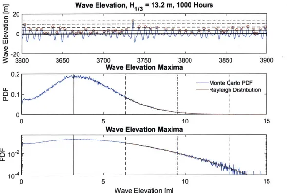
application is to produce a probability distribution function of the local maxima values and the local minima values. Figure 3-2 shows an example of these probability distribution functions for wave elevation maxima (wave peaks).

It has been shown that since the surface elevation is Gaussian, the local maxima

and minima (wave peaks and valleys) of this seaway will therefore follow a Rayleigh distribution [351. The Rayleigh distribution will only accurately capture this

behav-ior for the wave peaks and valleys that are somewhat away from the mean surface elevation. The Rayleigh distribution is plotted on Figure 3-2; on this and all future plots, the Rayleigh distribution is only be plotted for values more than two standard

deviations away from the mean. Quantities of interest which have a linear, time-invariant relationship with the incident surface elevation will also follow a Gaussian

Wave Elevation, 1/3 = 13.2 m, 1000 Hours

20

-20

S3600 3650 3700 3750 3800 3850 3900

Wave Elevation Maxima

0.2

-Monte Carlo PDF

o.1 Rayleigh Distribution

0

: 360 35 70 350 30I8030

I

0 5 10 15

Wave Elevation Maxima

10 -2

0102

0-0 5 10 15

Wave Elevation [m]

Figure 3-2: Probability distribution function for wave elevation maxima computed from Monte Carlo simulation of a seaway.

distribution, and have local maxima and minima which follow a Rayleigh distribu-tion when far enough away from the mean value. The degree of deviadistribu-tion from the

Rayleigh distribution in an output quantity of interest is an indication of the degree

of non-linearity in the system.

3.3

Extreme Value Theory

The problem with the Monte Carlo method is that accuracy of the probability is directly proportional to the number of observations. To obtain a quantity with a

probability of 0.10 requires 10 samples, 0.01 requires 100 samples, 0.001 requires

1,000 samples and so on. This becomes a huge issue when the calculations being

performed become complex and the amount of actual time required to perform the calculations for a simulated length of time begins to approach or exceed the simulated

of dice a million times in less than two seconds. If we pretend that the calculation was far more complex and instead the computer could only simulate rolling the dice ten times per second, the calculation would take more than two days. If a human can roll the dice once per second, this is still ten times faster than a human could have done it, but the convenience of a quick answer is lost.

One could certainly continue the Monte Carlo calculation and accept the long simulation time, but this is not an acceptable method in the fast paced and ever-changing world of ship design. There are two far more practical ways to proceed: the first method is the "brute force" approach which consists of applying more compu-tational resources to continue the Monte Carlo simulation; if run on ten computers, the calculation would take approximately two and a half hours instead of two days; a hundred computers could do the job in about fifteen minutes. The second option is to apply the principals of extreme value theory to the problem and extrapolate either simulation results, model test results, or actual data from a more manageable time scale.

Extreme value theory is perhaps most recognizable to an average people when it is used for insurance purposes. In the recent wake of Hurricane-Harvey, the media reported that the heavy rains produced a '500-year' flooding event, and in certain areas may have even been a '1,000-year' flooding event. The records for flooding events don't go back 1,000 years; in many places they don't even go back 100 years

121].

Instead these values are extrapolated from whatever data is available using extreme value theory.

Extreme value theory is a methodology for predicting the extreme events which lie in the tail of the probability distribution function. In practice, when a quantity of interest is analyzed, the Peaks in that quantity Over (or under) a certain Threshold (POT) are recorded and then a curve of best fit is applied with one of three possible tail structures: the Gumbel, Frkchet, or Weibull. Many of the variables of interest in ship design have been shown to generally follow the Weibull distribution

[8].

The extreme values of the quantity of interest are then extrapolated along the plot and used to determine the probability of the 'extreme events' in the tail of the probability

distribution function. The problem with this method is that anytime data is being extrapolated, there is a high risk of error: Hurricane Harvey was reported to be the third '500-year' flooding event to strike Houston in three years, which undermines any practical confidence in this label [21]. The horrific loss of property associated with this event demonstrates the possible consequences of under-designing a system

Chapter 4

Overview of Recent Work

4.1

Overview

Recent work by Mohamad and Sapsis at the MIT Stochastic Analysis and Non-Linear Dynamics (SAND) lab identified a different approach for quantifying extreme events

of systems subjected to irregular waves and coupled it with a sequential sampling algorithm which allows accurate results to be determined for meager computational

cost. This work is applicable to generic dynamical-stochastic systems and could theoretically be applied to numerous problems across many disciplines including naval

architecture, ocean engineering, climatology, chemistry, physics, finance, mechanical engineering, structural engineering, and many others. This chapter provides a brief

qualitative overview of this work, for technical details please see

[231.

4.2

Direct Extreme Event Quantification

The direct quantification method for extreme events in dynamical systems presented

is the Probabilistic Decomposition-Synthesis (PDS) framework and derives its name

from the way that the phase space is decomposed into intermittently unstable regions and system background stochastic attractors.

For a quantity of interest (eg. Force, Moment, etc.), it is assumed that the