Addressing two issues in machine learning : interpretability and dataset shift

Addressing Two Issues in Machine Lear '

MASACHUSETS (NSTITUTE

Interpretability and Dataset Shift

OF TECHNOLOGY

by

JUN 182

Fulton Wang

LIBRARIES

ARCHIVES

Submitted to the Department of Electrical Engineering and Computer

Science

in partial fulfillment of the requirements for the degree of

Doctor of Philosophy in Computer Science

at the

MASSACHUSETTS INSTITUTE OF TECHNOLOGY

June 2018

Massachusetts Institute of Technology 2018. All rights reserved.

Signature redacted

A uthor ...

Department of Electrical Engineering and Computer Science

May 23, 2018

Certified by...Signature

redacted

Cynthia Rudin

Associate Professor, Duke University

Thesis Supervisor

Signature redacted

Accepted by ...

liesliIkiolodziejski

Professor of Electrical Engineering and Computer Science

Chair, Department Committee on Graduate Students

77 Massachusetts Avenue Cambridge, MA 02139 http://libraries.mit.edu/ask

DISCLAIMER NOTICE

Due to the condition of the original material, there are unavoidable

flaws in this reproduction. We have made every effort possible to

provide you with the best copy available.

Thank you.

The images contained in this document are of the

best quality available.

Addressing Two Issues in Machine Learning: Interpretability and

Dataset Shift

by

Fulton Wang

Submitted to the Department of Electrical Engineering and Computer Science on May 23, 2018, in partial fulfillment of the

requirements for the degree of Doctor of Philosophy in Computer Science

Abstract

In this thesis, I create solutions to two problems. In the first, I address the problem that many machine learning models are not interpretable, by creating a new form of classifier, called the Falling Rule List. This is a decision list classifier where the predicted probabilities are decreasing down the list. Experiments show that the gain in interpretability need not be accompanied by a large sacrifice in accuracy on real world datasets. I then briefly discuss possible extensions that allow one to directly optimize rank statistics over rule lists, and handle ordinal data. In the second, I address a shortcoming of a popular approach to handling covariate shift, in which the training distribution and that for which predictions need to be made have different covariate distributions. In particular, the existing importance weighting approach to handling covariate shift suffers from high variance if the two covariate distributions are very different. I develop a dimension reduction procedure that reduces this variance, at the expense of increased bias. Experiments show that this tradeoff can be worthwhile in some situations.

Thesis Supervisor: Cynthia Rudin

Acknowledgments

I would like to thank my advisor Cynthia Rudin for all of her help, guidance, and

patience over the past years. She truly cares about her students, and does whatever it takes to help them. She has enabled my growth from an inexperienced researcher to a slightly more competent one, and for what I am eternally grateful. I would also like to thank my committee members Stefanie.jegelka and Pete Szolovits for their advice and feedback through this process. I have learned a lot from my labmates as well as outside collaborators Tyler McCormick, Daniel Neill, and Zhe Zhang. Much thanks must go to my friends both elsewhere and here, who have given ine support, guidance, and memories. Thank you to my parents Long-Ching and Shu-Min, who have been patient and understanding as I made my way through graduate school, and to my brother Edward, always willing to listen to my suggestions. Finally, thank you to my wife Carolyn, who has always put me above herself to support and motivate me, so that I could reach my full potential.

Contents

1 Falling Rule Lists 1.1 Introduction

1.2 Falling Rule Lists Model . . . . 1.2.1 Parameters of Model . . . .

1.2.2 Likelihood . . . .

1.2.3 Prior . . . . 1.3 Fitting the Model . . . . 1.3.1 Obtaining the MAP decision list 1.3.2 Obtaining the posterior . . . . . 1.4 Simulation Studies . . . . 1.5 Experiments . . . . 1.5.1 Predicting Hospital Readmissions 1.5.2 Performance on Public Datasets . 1.6 Conclusion

2 Extension of Falling Rule Lists

2.1 Introduction . . . . 2.2 Related Works . . . . 2.3 Formulation . . . . 2.3.1 Why Existing Rank Statistics Fail 2.3.2 Weighted Concordant Pairs . . . 2.3.3 Monotonicity Constraint... 2.4 Optimizing WCPa over Decision Lists .

with

. . . .

Stratification Models

. . . .

. . . .

. . . .

13 13 . . . . 16 . . . . . . 17

. . . .

..-

-..

.. . 1 17

. . . .

....

-

-.. .

.

18

. . ...21 . . I . . . . 21 . . . . 23 . . . . 27 . . . . . . . . 28 .. . . . . 28 . . . . 31 . . . . 32 33 33 36 36

38

38

39

2.4.1 Prefix Bound Algorithm . . . . . . 40

2.5 Experim ents . . . . . . .. . 41

3 Extreme Dimension Reduction for Handling Covariate Shift 45 3.1 Introduction ... ... 45

3.2 Background ... ... 47

3.2.1 Covariate Shift Problem ... ... 47

3.2.2 Importance Weighted Loss Minimization . . . .. 47

3.2.3 Density Ratio Estimation . . . . 47

3.3 Extreme Dimension Reduction ftr Importance Weighting . . . . 48

3.3.1 Motivation . . . ... .... 48

3.3.2 Formulation . . . . 49

3.3.3 Analysis of Dimension Reduction for Importance Weighting . . . 51

3.3.4 Solving the Optimization Problem . . . . 53

3.4 Simulation Study . . . ... . .. .. 54

3.4.1 Example with no estimator bias . . . . 54

3.4.2 Example with crippling estimator bias . . . . 57

3.5 Experiments with Real Data . . . . 59

3.5.1 Covariate Shift Experiments . . . . 59

3.5.2 Case Study on Learning Subgroup Models . . . . 62

3.6 Related W ork . . . . 65

3.7 Conclusion . . . . 66

List of Figures

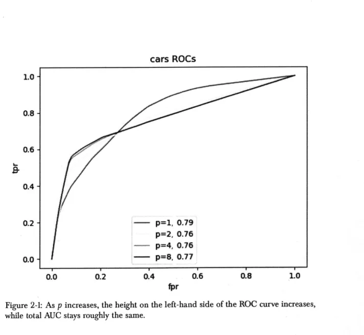
1-1 Mean distance to true list decreases with sample size . . . . .. 28 1-2 ROC curves for readmissions prediction. . . . . 30 2-1 As p increases, the height on the left-hand side of the ROC curve increases,

while total AUC stays roughly the same. . . . . 42

2-2 Comparison of model sparsity vs AUC for various models. . . . . 44

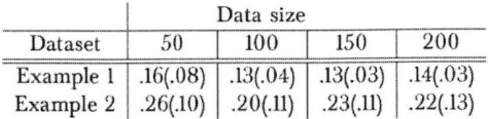
3-1 Example 1 -the relative importance between the only 2 predictive features is reversed between training & test distributions. Training points in red, test in blue. . . . . 56

3-2 Example 2 - P" is unchanged from before, so that X-) is still most predictive in the test distribution. Training points in red, test in blue. . , 58

3-3 Example 2 - Our method erroneously finds Xi and X2 to be equally

predictive in the test distribution. . . . . 58

3-4 For several datasets, the mean loss ("loss"), downstream effective sample

size ("N-eff"), and loss standard deviation (loss std") of our method is shown in black as the subspace dimension varies. The respective values of the unweighted and importance weighting baseline are shown in blue and red, respectively. Dataset dimension in parentheses. . . . . 60

3-5 Our method performs relative better when labelled data is scarce due to its ability to utilize more data for fitting. . . . . 63

List of Tables

1.1 Falling rule list for mammographic mass dataset. . . . . 14 1.2 Falling rule list for patients with no multiple readmissions history. . . . 29

1.3 AUROC values for readmission data . . . .3() 1.4 AUROC value comparisons over datasets . . . . 32 2.1 Stratification model for whether a treatment is positive, neutral, or negative. 34 2.2 Stratification model for whether a car is "good", for a(i) = i.. . . . . 44 2.3 Stratification model for whether a car is "good", for a(i).= P. .. ... 44 3.1 Example I - test loss over 50 replicates. . . . . 55 3.2 Comparison of our method's performance on the 2 simulated examples. 59

Chapter

1

Falling Rule Lists

1.1

Introduction

In healthcare, patients and actions need to be prioritized based on risk. The most at-risk patients should be handled with the highest priority, patients in the second at-risk set should receive the second highest priority, and so on. This decision process is perfectly natural for a human decision-maker - for instance a physician - who might check the patient for symptoms of high severity diseases first, then check for symptoms of less serious diseases, etc.; however, the traditional paradigm of predictive modeling does not naturally contain this type of logic. If such clear logic were well-founded, a typical machine learning model would not usually be able to discover it: most machine learning methods produce highly complex models, and were not designed to provide an ability to reason about each prediction. This leaves a gap, where predictive models are not directly aligned with the decisions that need to be made from them.

The algorithm introduced in this work aims to resolve this problem, and could be directly useful for clinical practice. A filling rule list is an ordered list of if-then rules, where (i) the order of rules determines which example should be classified by each rule (falling rule lists are a type of decision list), and (ii) the estimated probability of success decreases monotonically down the list. Thus, a falling rule list directly contains the decision-making process, whereby the most at-risk observations are classified first, then the second set, and so on. A falling rule list might say, for instance, that patients with a

IF IrregularShape AND Age 60 THEN malignancy risk is 85.22% 230

ELSE IF SpiculatedMargin AND Age > 45 THEN malignancy risk is 78.13% 64

ELSE IF ilDefinedMargin AND Age 60 THEN malignancy risk is 69.23% 39

ELSE IF IrregularShape THEN malignancy risk is 63.40% 153

ELSE IF LobularShape AND Density 2 THEN malignancy risk is 39.68% 63 ELSE IF RoundShape AND Age 60 THEN malignancy risk is 26.09% 46

ELSE THEN malignancy risk is 10.38% 366

Table 1.1: Falling rule list for mammographic mass dataset.

history of heart disease are in the highest risk set with a 7% stroke risk, patients with high blood pressure (who are not in the highest risk set) are in the second highest risk set with a 4% stroke risk, and patients with neither conditions of these are in the lowest risk set with a 1% stroke risk.

Table 1.1 shows an example of one of the decision lists we constructed for the mammographic mass dataset [271 as part of our experimental study. It took 35 seconds to construct this model on a laptop. The model states that if biopsy results show that the tumor has irregular shape, and the patient is over age 60, then the tumor is at the highest risk of being malignant (the risk is 85%). The next risk set is for the remaining tumors that have spiculated margins and are from patients above 45 years of age (the risk is 78%), and so on. The right column of Table 1.1 shows how many patients fit into each of the rules (so that its sum is the size of the dataset), and the risk probabilities were directly calibrated to the data.

Falling rule lists serve a dual purpose: they rank rules to form a predictive model, and stratify patients into decreasing risk sets. This saves work for a physician; sorting is an expensive mental operation, and this model does the sorting naturally. If one were to use a standard decision tree or decision list method instead, identifying the highest at-risk patients could be a much more involved calculation, and the number of conditions the most at-risk patients need to satisfy might be difficult for physicians to memorize.

Most of the models currently in use flr medical decision making were designed by medical experts rather than by data-driven or algorithmic approaches. These manually-created risk assessment tools are used in possibly every hospital; e.g., the TIMI scores,

Probability Support Conditions

CHADS2 score, Apache scores, and the Ranson score, to name a few

[6,

60, 33, 47, 45, 46, 7l.

These models can be computed without a calculator, making them very practical as decision aids. Of course, we aim for this level of interpretability in purely data-driven classifiers, with no manual feature selection or rounding coefficients.

Algorithms that discretize the input space have gained in popularity purely because they yield interpretable models. Decision trees [14, 68, 691, as well as decision lists 174], organize a collection of simple rules into a larger logical structure, and are popular despite being greedy. Inductive logic programming [61J returns an unstructured set of conjunctive rules such that an example is classified as positive if it satisfies any of the rules in that set. An extremely simple way to induce a probabilistic model from the unordered set of rules given by an ILP method is to place them into a decision list [e.g., see 28], ordering rules by empirical risk. This is also done in associative classification [e.g., see 82]. However, the resulting model cannot be expected to exhibit good predictive performance, as its constituent rules were chosen with a different objective.

Since it is possible that decision tree methods can produce results that are inconsistent with monotonicity properties of the data, there is a subfield dedicated to altering these greedy decision tree algorithms to obey monotonicity properties ill, 29, 41. Studies showed that in many cases, no accuracy is lost in enforcing monotonicity constraints, and that medical experts were more willing to use the models with the monotonicity constraints

[65].

Even with (what seem like) rather severe constraints on the hypothesis space such as monotonicity or sparsity in the number of leaves and nodes, it still seems that the set of accurate classifiers is often large enough so that it contains interpretable classifiers [see 36]. Because the monotonicity properties we enforce are much stronger than those of (author?) [11, 29, 4] (we are looking at monotonicity along the whole list rather than for individual features), we do find that accuracy is sometimes sacrificed, but not always, and generally not by much. On the other hand, it is possible that our method gains a level of

practicality and interpretability that other methods simply cannot.

no matter how one measures it in one domain, it can be different in the next domain. A falling rule list used in medical practice has the benefit that it can, in practice, be as sparse as desired. Since it automatically stratifies patients by risk in the order used for decision making, physicians can choose to look at as much of the list as they need to make a decision; the list is as sparse as one requires it to be. If physicians only care about the most high risk patients, they look only at the top few rules, and check whether the patient obeys any of the top clauses.

The algorithm we provide for falling rule lists aims to have the best of all worlds: accuracy, interpretability, and computation. The algorithm starts with a statistical assumption, which is that we can build an accurate model from pre-mined itemsets. This helps tremendously with computation, and restricts us to building models with only interpretable building blocks Isee also 51, 87J. Once the itemsets are discovered, a Bayesian modeling approach chooses a subset and permutation of the rules to form the decision list. The user determines the desired size of the rule list through a Bayesian prior. Our generative model is constructed so that the monotonicity property is fully

enforced (no "soft" monotonicity).

The code for fitting falling rule lists is available online.

1.2 Falling Rule Lists Model

We consider binary classification, where the goal is to learn a distribution p(Ylx), where Y is binary. For example, Y might indicate the presence of a disease, and x would be a patient's features. We represent this conditional distribution as a decision list, which is an ordered list of IF...THEN... rules. We require a special structure to this decision list: that the probability of Y = 1 associated with each rule is decreasing as one moves down the decision list.

We use a Bayesian approach to characterize the posterior over falling rule lists given training data D = {(x, Yn} ..,N (of size N), x,, E X, the patient feature space, hyperparameters H, and y, E (0, 1}. We represent a falling rule list with a set of

parameters 0, specify the prior po(-;H) and likelihood py({yj}I0;{x, }), and use simulated annealing and Monte Carlo sampling to approximate the MAP estimate and posterior over falling rule lists,

1.2.1 Parameters of Model

A falling rule list is parameterized by the following objects:

L E Z+ c

(-) E BX (-),

for

IO

= ... - 1

r

1

e

IR, for = 0,..., L (size of list) (F clauses) (risk scores) such that rl. 1 ; rj for I = 0,..., L - I (monotonic) (1.4)

where Bx(-) denotes the space of boolean functions on patient feature space X. Bx(.) is the space of possible IF clauses; cI(x) will be I if x satisfies a given set of conditions. For this work, we will not assume L, the size of the decision list, to be known in advance. The value of i will be fed into the logistic function to produce a risk probability between 0 and 1. Thus, co(-) corresponds to the rule at the top of the list, determining the patients with the highest risk, and there are L + 1 nodes and associated risk probabilities in the list: L associated with the c(-)'s, plus one for default patients - those matching none of the L rules.

1.2.2

Likelihood

Given these parameters, the likelihood is as follows: Given L, let Z(x;

{cI(-)}).)X

-+

10,...,

L}

be the mapping from feature x to the index of the length L rule list it "belongs

(1.1)

(1.2)

(1.3)

to (equals L for default patients):

Z(x; {ci()}_-

)

=

(.5)

L

if c(x)=0

for I=0,...,L-1 min(l : c,(x) = 1,

1

= 0,..., L - 1) otherwise. Then, the likelihood is:

y,,jL, {c;(-)}f;_-, Irn;fl

x-Bernoulli(logistic(r _)), where (1.6)

Zn = Z(xn;{ci()} ). (1.7)

1.2.3

Prior

Here, we describe the prior over the parameters L, {cj}4- ,{r} _ . We will provide a reparameterization that enforces monotonicity constraints, and finally give a generative model for the parameters.

As discussed earlier, to help with computation, we place positive prior probability of {cjL}1 only over lists consisting of boolean clauses B returned by a frequent itemset mining algorithm, where for c(-) e B, we have c(.): X -+ (0, 11. For this particular work we used FPGrowth [13], whose input is a binary dataset where each x is a boolean vector, and whose output is a set of subsets of the features of the dataset. For example, x2 might

indicate the presence of diabetes, and x, 5 might indicate the presence of hypertension,

and a boolean function returned by FPGrowth might return 1 for patients who have diabetes and hypertension. It does not matter which rule mining algorithm is chosen because they all perform breadth-first searches to return a set of clauses that have sufficient support. Here, B needs to be sufficiently large, so that the hypothesis space of considered models is not too small. B can be viewed as a hyperparameter, and the maximum length a decision list can have under our model is IBI, the number of rules in

Reparameterization

To ensure the monotonicity constraints that r, r- for I = 1 ... L in the posterior, we

choose the scores r; to, on a log scale, come from products of real numbers constrained to be greater than 1. That is, conditioned on L, we let

r, = log(vi) for

l=0,...,L

(1.8)

vt = KHfr11 Y; for

I

= 0,..., L -1 (1.9)

vj= K

(1.10)

and require that

y" > I for I = 0,..., L - I (L.I)

K > 0, (1.12)

so that rL, the risk score associated with the default rule, equals logK. The prior we

place over

{y}

;~ and K will respect those constraints.

Thus, after reparameterizing, the parameters are

y =

Lc

1

(-)

,

jy;}

,K}

(1.13) Prior Specifics

The prior over parameters L,

{c1()}

,yfr } K is generated through the following

process:

1. Let hyperparameters

lIBI-I JBj-I A- 1 H= {B,{a;I{

=

, ;}0

,aK1K,

WII0

)

be

given.

2. Initialize 0 - {}.

3. Draw L ~Poisson( A).

c;( - PC(-

(-10;

B,{jwj}72

(1.14

P.)

(c(.)

=

c (-)I9; B, {IW ;1'

)

(1.15)

-c Wj if

c_() i 0

and 0 otherwise. (1.16)

Update ) <- E U

{c,(-).}

(1.17) 5. For I = 0,..., L - I draw yj ~ Gamma I(a,,

P1),

which is a Gamma distribution trun-cated to have support only above 1.

6. Draw K ~ Gamma(aK3K).

We now elaborate on our choice for each involved distribution. We let L - Poisson(A), where A reflects the prior decision length desired by the user. We let c1(.) be the result of a

draw from a discrete distribution over the yet unchosen rules, B\

{c(-)}> ,

where the 1-th rule is drawn with probability proportional to a user designed weight wl. For example, a rule might be chosen with probability proportional to the number of clauses in it. This allows the user to express preferences over different types of clauses in the list. Given L, only

{c(.);}r1

are observed, though note this process specifies a joint distribution over all of

{c(-);

}'. Letting {lyl},_~ to be independently distributed truncated gamma variables permits posterior Gibbs sampling while enforcing the monotonicity constraints and still permitting diversity over prior distributions. For example, one could encourage some of the y's near the middle (of L) of the list to be large, in which case the risks would be widely spaced in the middle of the list (but this would force closer spacing at the top of the list where the risks concentrate near 1). Finally, K, which models the risk of patients not satisfying any rules, is Gamma distributed.

1.3

Fitting the Model

First we describe our approach to finding the decision list with the maximum a posteriori probability. Then we discuss our approach to perform Monte Carlo sampling from the posterior distribution over decision list parameters

0

= IL, CO,.,L_1

(),K,

Yo,,_I} as

described in Equation (113),

ppost(L, CO,..jL_.

(-),K,

yo,...._|Iy1,...,N'X ,..,N)-

(1.18)

1.3.1

Obtaining the MAP decision list

We adopted a simulated annealing approach to find 0* = L*, C,..L1 (.),K*, yU,.., ),

where

*,

c

_(.),K*, y* ,._ (1.19)

E argmaXL~. .g (K,yo -1

where C is shorthand for the unnormalized log of the posterior given in Equation (1.18). We note that the optimization problem in Equation (1.19) is equivalent to finding:

VPCc ,L- I_(-)T (1.20)

E argmaxL- (L,

{CIL4

C(.L-1 , K*, y

where

Ky (1.21)

E argmax ,y L,;) , .,

Note that K* and y._ depend on L,

{ci(.)}=-.

Furthermore, the solution to the subproblem of finding K* and y. can be ap-proximated closely using a simple procedure, as it involves maximizing the posterior probability of a decision list given the rules {c(-)} _~ . Optimizing Equation (1.20) lends

itself better to simulated annealing than Equation (1.19); optimizing (1.20) involves opti-mization over a discrete space, namely the set and order of rules c1(.). In this formulation,

at each simulated annealing iteration, we need to evaluate the objective function for the current rule list

Ic,(.))fL-

, which involves solving the continuous subproblem of finding

the corresponding K* and y _1.

Given an objective function E(s) over discrete search space S, a function specifying the set of neighbors of a state N(s), and a temperature schedule function over time steps, T(t), a simulated annealing procedure is a discrete time, discrete state Markov Chain

Ist}

where at time t, given the current state st, the next state St+ is chosen by first randomly selecting a proposal 3 from the set N(s), and setting s+ 1 = s with probability

rnin(l,exp(- E )), and s.. = s otherwise.

The search space of the optimization problem of Equation (1.20) is L,

{c(_)}1

the

set of ordered lists of rules drawing from the finite pre-mined set of rules B. Based on Equation (1.20), we let

E

=

-=

(L,cI()1~

,K*, _1).

(1.22)

We simultaneously define the set of neighbors and the process by which to randomly choose a neighbor through the following random procedure that alters the current rule list {c;(-)}I_~ to produce a new rule list {c;(.)}-' (The new list's length may be different): Choose uniformly at random one of the following 4 operations to apply to the current rule list,

{c(-)}

₁

:

1. SWAP: Select i 0

j

uniformly from 0,..., L - 1, and swap the rules at those 2 positions, letting c;(.) <- cj(-) and 6;()+- c-).

2. REPLACE: Select i uniformly from 0,..., L - 1, draw c(.) from the the distribution

pe)(-; B,{w;}J ) defined in Equation (1.16), where 8 = {c(-)}j i-_i 0,_,_1 and set '.(.) +- c(.).

a rule c(-) from pc(.)(-le;B, {w} I 1"- ), where

E=

{C()} ,L1, and insert it at the

chosen insertion point, so that L <- L + 1.

4. REMOVE: Choose i uniformly at random from 0,..., L - 1, and remove c;(-) from the current rule list, so that L <- L -1.

Note that this approach optimizes over the full set of rule lists from itemsets, and does not rely on greedy splitting. Even Bayesian tree methods that aim to traverse a wider

search space use greedy splitting and local solutions, e.g. (author?)

[191.

1.3.2 Obtaining the posterior

To perform posterior sampling, we use Gibbs sampling steps over {y;}f-r and K made possible by variable augmentation, and Metropolis-Hastings steps over L and (c(.)). We describe the variable augmentation step, the schedule of updates we employ, and finally the details of each individual update step.

Augmenting the model with two additional variables U, C, for each n = 1,..., N pre-serves the marginal distribution over the original variables, and enables Gibbs sampling over K and each yj [see 26]:

,, - Exponential(f1)

Un

~

Poisson(,

) Yn = 1 (Un > 0) for n = N for n = ,...,N for n = ,...,N.

Marginalizing over (, we see that in this augmented model, y, ~ Bernoulli(logistic(r ,)),

(1.23)

(1.24)

as before:

P(yn = 1) = P(Un > 0)

(1.26)

= 1

f

p(Un = 0jC.)p((,JdCn

(1.27)

=

1f

exp(-(v_,)

exp(-Cn)dGC

(1.28)

=1- (0 + V_ )- (1.29) (1.30) 1+exp(r ,) Schedule of Updates

Given the augmented model, we cycle through the following steps in the following deterministic order. These will each be discussed in detail shortly. Regarding no-tation, we will use use 0aug to refer to the parameters of the augmented model:

(L,IcI(-)}f-

,LK,{y')fi,{U } ,{)

),

so that Gibbs updates can be described more

succinctly.

Step I (Gibbs steps for each yj):

Sample

';

Py(-(0aug \ y;) fn} N xI V )

for I = 0,..., L - 1.

Step 2 (Gibbs step for K):

Sample

k-

~PK ( (Oaug \ K),{Yn} N:;{Xn}INI).

Step 3 (Collapsed Metropolis Hastings Step):

Perform Metropolis-Hastings update over (L, (c;(-)}

Z-),

under the original model from Equation (1.18). This can be viewed as a collapsed Metropolis-Hastings step, where the collapsed parameters are the augmenting variables

IUi}

I,{,} }%;.

Step 4 (Gibbs step for

({1N.,{U};

)):

Jointly sample

Mixing Gibbs and collapsed Metropolis-Hastings sampling steps requires special care to ensure the Markov chain is proper in that it possesses the desired stationary distribution. We refer to (author?)

184]

for details, but do note that after the collapsed Metropolis-Hastings step, first performing a Gibbs update of {C n=,, and then a separate

Gibbs update for

I

U}

IN (or in reverse) would not have been proper.

Update Details

XWe now elaborate on each step of the update schedule:

Step I In this augmented model, the full conditional distribution of each y7 is Gamirna distributed, so that it can be sampled from directly. Let, for 1 = 0,..., L - I

S

Kf

.jy

for

0

k (.1

Cak=

0

for I <k L.

Then, it can be derived that

YI I(aug \

Y')

I{nj I

}=

1xn=₁ (1.32)

N N

Gamma

al

+ z & l U<n,f+ +,

n=1 n=1

where aj,p; govern the prior of yj and z, as described in Equation (1.7) denotes the rule a datum belongs to.

Step 2 Similarily, let

rlk

giy

for

0

<

k

< L - I

0k{1 k

(1.33)

Then

KI(Oaug \ K),{y1 )xn=i (1.34)

N N

Gamma aK PK

+

L

noz,,

(1.35)

n=1 +n=1

Step 3 The reason for using a collapsed rather than regular Metropolis-Hastings step

was to improve chain mixing. The Metropolis-Hastings proposal distributions over

(L,ci(-)}.

)

are exactly as in the proposal distribution used to generate a successor state in the simulated annealing we used to find the MAP decision list. The only difference is that if the ADD operation is chosen and a rule c(.) inserted at position k in the rule list,

then sample

)k

-

Gamma(akPk), the prior distribution of yk, and insert it at position

k in (yj' . Thus, we simply provide the Metropolis-Hastings

Q

probabilities. For simplicity, we do so for the case when the weights (w} associated with each c(.) B are equal. (L)( BL) ADD if REPLACE _ L~) -(RBFVL)L

Q({

e(_))

;c; (.)}, )

if REMOVE 2 _{if SWAP.} L(L-1)

Step 4 In the full conditional distribution of ({ N 1,{ U}N 1), the set of pairs of variables, i(U,,,)}>1 is mutually independent, due to conditioning. Therefore to

sample from it, it is sufficient to independently sample (Un, n for n = 1,...,N. It can be shown that the following sampling scheme samples from the full conditional distribution: For n = 1,...,N, if y, = 0, set Ul = 0 and sample

Otherwise, sample

D/ ~1 + Geometric , then (1.37)

.1I+ VZH.,

&v

~ Gamma

(1

+

Oi,:,

I + vz ,).

(1.38)

1.4 Simulation Studies

We show that for simulated data generated by a known decision list, our simulated annealing procedure that searches for the MAP decision list, with high probability, recovers the true decision list.

Given observations with arbitrary features, and a collection of rules on those features, we can construct a binary matrix where the rows represent observations and the columns represent rules, and the entry is 1 if the rule applies to that observation and 0 otherwise. We need only simulate this binary matrix to represent the observations without losing

generality. For our simulations, we generated independent binary rule sets with 100 rules

by setting each feature value to 1 independently with probability 0.25.

We generated a random decision list of size 5 by selecting 5 rules at random, and

setting the yo,..., ),s so that the induced po., p5 were roughly evenly spaced on the unit

interval: (.84,.70,.54,.40,.25,.14). For each N, we performed the following procedure

100 times: generate the random rule matrix, random decision list, and assign it the

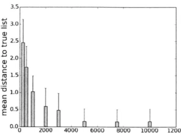
aforementioned {y4}, obtain an independent dataset of size N by generating labels from this decision list, and then perform simulated annealing using the procedure described in Section 1.3.1 to obtain a point estimate of the decision list. We then calculate the edit distance of the decision list returned by simulated annealing to the true decision list. Figure 1-1 shows the average distance over those 100 replicates, for each N. We ran simulated annealing for 5000 steps in each replicate, and used a gradual cooling schedule.

0 U a 4.J L, E 3.5 3.0k 2.0 1.0 0.s1. 0.0 0 2000 4000 6000 8000 10000 12000

Figure 1-1: Mean distance to true list decreases with sample size.

1.5

Experiments

Our main experimental result is an application of Falling Rule Lists to predict 30 day hospital readmission from an ongoing collaboration with medical practitioners [details to appear in 23].

Since we placed an extremely strong restriction on the characteristics of the predictive model (namely the monotonicity property, sparsity of rules, and sparsity of conditions per rule), we expect to lose predictive accuracy over unrestricted methods. The interpretability benefit may or not be sufficient to compensate for this, but this is heavily application-dependent. We have found several cases where there is no loss in performance (with a substantial gain in interpretability) by using a falling rule list instead of, say, a support vector machine, consistent with the observations of [361 about very simple classifiers performing well.

Later in this section, we aim to quantify the loss in predictive power from Falling Rule Lists over other methods by using an out-of-sample predictive performance evaluation. Specifically, we compare to several baseline methods on standard publicly available datasets to quantify the possible loss in predictive performance.

1.5.1

Predicting Hospital Readmissions

We applied Falling Rule Lists to preliminary readmissions data being compiled through a collaboration with a major hospital in the

U.S.

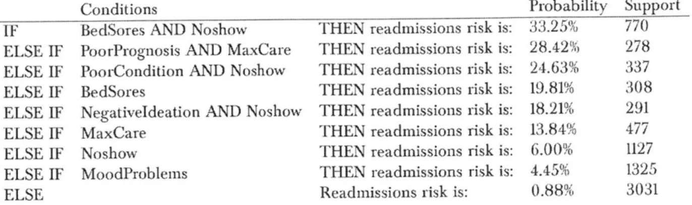
[23], where the goal is to predict whether a

IF BedSores AND Noshow THEN readmissions risk is: 33.25% 770

ELSE IF PoorPrognosis AND MaxCare THEN readmissions risk is: 28.42% 278 ELSE IF PoorCondition AND Noshow THEN readmissions risk is: 24.63% 337

ELSE IF BedSores THEN readmissions risk is: 19.81% 308

ELSE IF NegativeIdeation AND Noshow THEN readmissions risk is: 18.21% 291

ELSE IF MaxCare THEN readmissions risk is: 13.84% 477

ELSE IF Noshow THEN readmissions risk is: 6.00% 1127

ELSE IF MoodProblems THEN readmissions risk is: 4.45% 1325

ELSE Readmissions risk is: 0.88% 3031

Table 1.2: Falling rule list for patients with no multiple readmissions history.

patient will be readmitted to the hospital with )30 days, using data prior to their release. The dataset contains features and binary readmissions outcomes for approximately 8,000 patients who had no prior history of readmissions. The features are very detailed, and include aspects like "impaired mental status," "difficult behavior," "chronic pain," "feels unsafe" and over 30 other features that might be predictive of readmission. As we will see, luckily a physician may not be required to collect this amount of detailed information to assess whether a given patient is at high risk for readmission.

For these experiments and the experiments in the next section, no parameters were tuned in Falling Rule Lists (FRL), and the global hyperparameters were chosen as follows. We mined rules with a support of at least 5% and a cardinality of at most 2 conditions per rule. We assumed in the prior that conditioned on L, each rule had an equal chance of being in the rule list. We set the prior of (yi J(L to have noninformative and independent distributions of gamma(1,0.1), and the prior expected length of the decision list, A, to be 8. We performed simulated annealing search for 5000 steps with a constant temperature of 1 for simplicity.

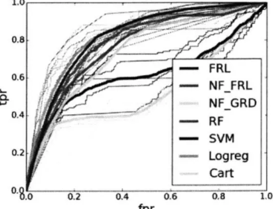
We measured out-of-sample performance using the ALROC from 5-fold cross valida-tion where the MAP decision list from training was used to predict on each test fold in turn. We compared with SVM (with Radial Basis Function kernels), [2 regularized logistic

regression (Ridge regression, denoted LogReg), CART, and random forests (denoted RF), implemented in Python using the scikit-learn package. For SVM and logistic regression, hyperparameters were tuned with grid search in nested cross validation.

Method I Mean AUROC (STD) FRL .80 (.02) NE_FRL .75 (.02) NFGRD .75 (.02) RF .79 (.03) SVM .62 (.06) Logreg .82 (.02) Cart .52 (.01)

Table 1.3: AUROC values for readmission data

1.0- 0.8-0.6 - -- NFFRL - NF_GRD 0.4 - - --. 0.2- Logreg Cart 0 02 0.4 0.6 0.8 10 fpr

Figure 1-2: ROC curves for readmissions prediction.

As discussed, decision lists consisting of rules from an inductive logic programming method are not expected to exhibit strong performance. We tested nFoil [501 with the default settings (max number of clauses set to 2) to obtain a set of rules. These rules were ordered in two different ways, to form two additional comparison methods: 1. by the empirical risk of each rule (denoted NFGRD), and 2. by using the set of rules as the pre-mined rule set that FRL accepts as input (denoted NFFRL). Note that the risk probabilities in rule lists returned by NFGRD are not necessarily decreasing monotonically, and that not all of the nFoil rules are necessarily in the rule list returned by NFJRL, since omission of a rule can increase the posterior.

The AUROC's for the different methods are in Table 1.3, indicating that there was no loss in accuracy for using Falling Rule Lists on this particular dataset. For all of the training folds, the decision lists had a length of either 6 or 7 - all very sparse.

are bolded. For this particular dataset, SVM RBF and CART did not perform well. It is unclear why SVM did not perform well, as cross-validation was performed for SVM; usually SVM's perform well when cross-validated (though it is definitely possible for them to have poor performance on some datasets - on the other hand, CART often performs poorly relative to other methods, in our experience). As expected, the nFoil-based methods exhibited worse performance than our falling rule list method. FRL performed on par with the best method, despite its being limited to a very small number of features with the monotonic structure.

Table 1.2 shows a point estimate obtained from training Falling Rule Lists on the full dataset, which took 88 seconds. The "probability" column is the empirical probability of readmission for each rule; "support" indicates the number of patients classified by that rule.

The model indicates that patients with bed sores and who have skipped appointments are the most likely to be readmitted. The other conditions used in the model include "PoorPrognosis" meaning the patient is in need of palliative care services, "PoorCondition" meaning the patient exhibits frailty, signs of neglect or malnutrition, "Negativeldeation" which means suicidal or violent thoughts, and "MaxCare" which means the patient needs maximum care (is non-ambulatory, confined to bed). This model lends itself naturally to decision-making, as one need only view the top of the list to obtain a characterization of high risk patients.

1.5.2

Performance on Public Datasets

We performed an empirical comparison on several UCI datasets 110], using the above experimental setup. This allows us to quantify the loss in accuracy due to the restricted form of the model.

Table 1.4 displays the results. As discussed earlier, we observed that even with the severe restrictions on the model, performance levels are still on par with those of other methods, and not often substantially worse. This is likely due to the benefits of not using a greedy splitting method, restricting to the space of mined rules, careful formulation, and optimization.

Furthermore, FRL beats the nFoil based methods in performance on all the public datasets. Again, the reason is that the set of rules from nFoil was found using a different objective, not intended to predict well when placed into a decision list. Even with NFFRL, where any subset of the nFoil rules could be selected and placed in any order, performance was poor, showing the nFoil rule set did not contain rules that were useful for a falling rule list. The set of nFoil rules was always much smaller than those from FPGrowth (see supplement), overly restricting the hypothesis space.

1.6

Conclusion

We present a new class of interpretable predictive models that could potentially have a major benefit in decision-making for some domains. As nicely stated by the director of the U.S. National Institute ofJustice [731, an interpretable model that is actually used is better than one that is more accurate that sits on a shelf. We envision that models produced

by FRL can be used, for instance, by physicians in third world countries who require

models printed on laminated cards. In high stakes decisions (like medical decisions), it is important we know whether to trust the model we are using to make decisions; models like FRL help tell us when (and when not) to trust.

Method

I

Spai Mamm Breast Cars

FRL

i

.91(.Ol)

.82(.02)

.95(.04)

.89(.08)

NFFRL .90(.03) .67(.03) .70(.11) .60(.21) NF_GRD .91(.03) .72(.04) .82(.12) .62(.20)

SVM

.97(.03)

.83(.01)

.99(.01)

.94(.08)

Logreg .97(.03) .85(.02) .99(.01) .92(.09) CART .88(.05) .82(.02) .93(.04) .72(.17)

RF

.97(.03)

.83(.01)

.98(.01)

.92(.05)

Chapter 2

Extension of Falling Rule Lists

2.1

Introduction

Falling Rule Lists gave a way to rank individuals by priority - the individuals captured

by the top rule are those of highest priority, those captured by the 2nd rule are of the

2nd highest priority, etc. However, they have 2 shortcomings. Firstly, they do not directly optimize rank statistics like the AUC or variants that emphasize the top of the ranking. Thus, they are not as flexible as we would like. Secondly, Falling Rule Lists cannot handle

ordinal data. In this section, we present a formulation to learn rule lists, which still ranks individuals in order of priority, while addressing these two shortcomings.

Medical studies often use area under the ROC curve (AUC), or other rank statistics such as partial AUC

124,

39], to measure the quality of their risk predictions. Thus, it is

natural to create risk strata that are optimal in terms of rank statistics. In this work, we will consider both the scenario when labels are binary, so that the strata are risk strata, and the more general case when the labels are ordinal, so that our goal is what we term "ordinal stratification".

Several challenges arise when optimizing rank statistics, which is the central challenge for learning-to-rank (supervised ranking) problems [53, 62, 75, 2, 8, 21, 91, 32, 70, 161. Recent work in this area [76J has showed that conditional linear rank statistics yield trivial solutions when directly optimized, and that convexifications of these rank statistics fail to optimize the rank statistics themselves. (author?)

176]

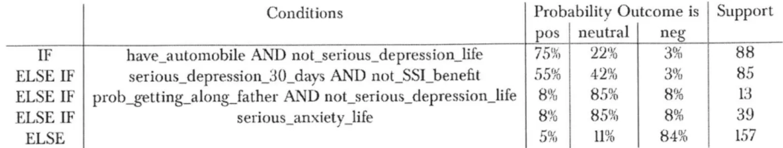
introduce a new class of rank

Conditions Probability Outcome is Support

pos | neutral neg

IF haveautomobile AND notserious depressionlife 75% 22% 3% 88

ELSE IF seriousdepression_30_days AND notSSIbenefit 55% 42% 3% 85

ELSE IF prolbgetting-alongjather AND notserious-depressionlife 8% 85% 8% 13

ELSE IF seriousanxietylife 8% 85% 8% 39

ELSE 5% 11% 84% 157

Table 2.1: Stratification model for whether a treatment is positive, neutral, or negative. statistics that is designed to be optimized; however, this class of rank statistics was not designed to be used with stratification models, where multiple individuals are assigned to the same stratum. As we will show in this work, their class of rank statistics does not pass basic sanity checks in the case of stratification, for instance, even strata that perfectly group and sorts individuals by their ordinal label do not always achieve the highest rank statistics.

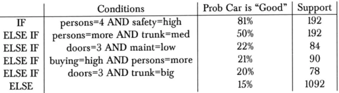
We utilize a class of rank statistics, an application of weighted Kendall's tau [90, 441 related to conditional linear rank statistics of [201, and an algorithm to optimize them to produce ordinal stratification models. A ordinal stratification model is a rule list, or decision list, but it does not group together observations with the same outcomes like a standard decision tree or predictive model. Instead it places patients within several stratum (e.g., high, medium, low risk). Each strata contains a range of labels; when labels are binary, a high risk stratum might contain individuals with risk 90% for having a disease, and when labels are ordinal, a high ranking stratum might contain individuals whose credit scores are between 750 and 850. Because of our learning-to-rank formulation, our algorithm is able to produce stratification models that are flexible (optimize a wide variety of rank statistics) and interpretable (containing few strata). An example of a stratification model is in Figure 2.1. The outcome can take on 3 ordinal values: whether a given treatment for reducing drug usage is positive, neutral, or negative. The decision stratifies and ranks individuals by conditions, so that the individuals captured by rules high in the list will have to have values of the ordinal outcome.

2.2

Related Works

As discussed above, stratification models are different than other predictive models, in that, given a stratum, there is no single prediction, instead each stratum contains a range (e.g., one stratum contains observations of which 90% have a positive label). If we would like to rank statistics that focus heavily at the top of the ranked list [see 391, for an optimal sparse risk stratification model, there may be more strata to represent the higher risk categories, and fewer strata to represent low risk categories. To judge the quality of a risk stratification model, we introduce rank statistics that consider pairs of observations

(crucialpairs, as used within RankBoost

1321),

where observations in each pair are within

different strata. This is useful because we do not want to compare labels of observations that are all within, for instance, the "low risk" stratum.

Usually optimization of rank statistics are handled by approximating the rank statistic with a convex proxy, as RankBoost does, which leads to easier optimization for linear or kernel models, but convex proxies have several disadvantages [761, for instance that they are not good approximations of the underlying rank statistic of interest. For optimizing rule lists, there is no advantage to using convex proxies, and recent work on rule lists

[? ] has shown that it is possible to produce rule lists that are certifiably optimal

within reasonable time limits, indicating that approximate solutions are likely to produce almost-optimal rule lists.

Learning-to-rank can be used for high-stakes prioritization problems, such as airline fleet maintenance [63J and lead paint inspections in dwellings [661. Standard learning-to-rank techniques would produce only a ranked list, not a reason for the ranking. In both cases, risk stratification models that focus on the more high risk units would be potentially useful; airline maintenance crews could more easily prioritize repairs, knowing why these planes should be prioritized, while lead paint inspection crews could prioritize

2.3

Formulation

The training data are N labelled observations

{xi,yj

with Xi E {0, 1)D and Y; E

Y,

an ordinal set. We will map each xi to

Z;

E [L], where L E Z" , so that zi

}

places the training data into L ordered strata. This mapping will be through a function

f,

represented as a decision list with some sequence of rules ro...r. 1, where

r

E [D]. We represent the set of

rules the decision list can contain with a member of [D] because each rule is identified with one of the D binary features. Formally,

f(x;; L, ro...rL_1) = L - min{Il : xi = 1} if i i I(ro...rL1_), 0 otherwise, (2.1) where I(rO...r_1):= {i : X iX = 0}, i.e. individuals for no rule in the given decision

list is true, so that they they are given the lowest priority of 0. Note that the rules in a given decision list are numbered so that ro and rL_1 are the rules at the top and bottom of the decision list, respectively.

xi for which z = f(x;) is larger, i.e. "captured" by a rule high in the list, are

interpreted to have higher priority. To formalize the desiderata that individuals with higher ordinal labels should be assigned higher priority, we need to define a rank statistic that captures the extent to which that is true. A rank statistic is a function of the ordering of individuals induced by the assigned priorities (f(xi)} relative to that of the true ordinal labels {yj}. We can thus generically write the optimization problem by which we choose a rule list as maxLr ..r R({f(x;; L, ri...rL)},

}

}) - AL where R(.,.) denotes a generic rank

statistic. The parameters of the problem are the length of the decision list and the rules in it. AL is regularization on the complexity of the decision list as measured by its length, so that the training value of the rank statistic would represent the expected rank statistic over a new sample drawn from the training distribution.

2.3.1

Why Existing Rank Statistics Fail with Stratification Models

The setting we consider is unique in that both the learned ranking function (because the decision lists groups individuals into ordered strata) and the true ranking (because the

labels are ordinal) can have ties. In choosing a rank statistic R to optimize under this setting, a basic sanity check it should pass is that the rank statistic is maximized when the asserted and true ranking perfectly agree. That is, if Y = [L], it should be the case that

{yj}

e argmaxlz:::EL R({z;}, {y;). Unfortunately, a recently proposed wide class of

rank statistics does not satisfy this sanity check.

Conditional linear rank statistics (CLRS)

120]

encompass many widely used rank statistics, including AUC, DCG, and were originally designed for the binary label setting. Given an non-decreasing function a(.) : -R -+, the corresponding CLRS is defined

to be CLRSa({Zi},il) Ejyja(Ej][z; >

z1]).

1761

showed that when CLRS are directly optimized, a trivial solution for which the f(x:) are assigned to the same constant is returned. As we directly will optimize rank statistics, CLRS would not be suitable. They propose subrank CLRS, defined as CLRS,"b := Tj y a(LE 1[z; > zi]), whose optimization no longer returns trivial solutions. Note the > instead of >. However, subrank CLRS does not pass the aforementioned sanity check.

We first present a simple example to illustrate. Suppose a(r)= r, and yj = y-2 =

1, y3 = 1,y4 1, y = 1 Suppose the asserted ranking perfectly agrees with the labels, i.e.

z; = Y; for i =

5.

Then CLRSUb({z;},{y) =0 + I + I + I + = 4. Now consider a different asserted ranking {z'}, where z' = 0, z = 0, z = 1 ,z'= 1. That is, individual 2 has been moved to the lower of the 2 strata.CLRSUb({zi}, {yj

})

= 0 + 0+ 2+ 2+2 = 6. By

moving a positive individual to the lower strata, the subrank of the positive individuals still in the higher strata was increased. This phenomenon is true in general:

Lemma 2.3.1. ForailL, nondecreasinga(-), exists (yj s.t. {y;j i argmaxlza CLRS'1b({zI} {;})

The reason subrank CLRS fails the sanity check is that when the asserted ranking can

have ties, the subrank of an individual does not reflect how well ranked that individual is relative to others, as subrank does not depend on the true labels. Subrank CLRS sufficed when the asserted rankings did not have ties, because the subranks over the dataset was exactly equal to [NI, so that a good ranking would allocate the high subranks to the true positive individuals.

2.3.2

Weighted Concordant Pairs

The rank statistic family we propose to maximize is a generalization of the rank statistics based on pairwise agreements between the asserted and tree ranking. We call this family weighted concordant pairs. Members of the family are parametrized by a non-decreasing

and convex function a(-): IR+ -_- + defined as

WCPa(Izi},{JY}):=

a(Zi[z;

>Lzj[y >yI)

(2.2)

When a(.) is the identity, WCPa reduces to the standard pairwise ranking error that Rankboost approximates. The steepness of a(-) controls the emphasis placed on properly ordering the individuals that are truly top ranked. When a(-) is very steep, an asserted ranking

{z;}

would achieve a high WCPa by assigning high z; to the truly top ranked individuals, even if at the expense of misranking lower ranked individuals. In this work we will assume a(.) is of the form a(i)= i P for some p > 1.

Because a(-) is assumed convex, the following desirable property holds for any WCPa:

Lemma 2.3.2. For any tyji,L E Z+ there exists Jz;} E argmax,, V[LWCPa({Z {I;})

such that

for any

yi, I{I

:

3z,

:

yj

=

yi,z = I}I

1.

That is, the set of ordered stratum of size L maximizing WCPa contains an ordered strata in which for every label, individuals with that label all belong to the same stratum. In the special case when Y = [L], Lemma 2.3.2 implies that WCPa passes the sanity

check that CLRSlub failed: {y;} E argmax1 WCPa({Zi},{ i}).

Given the favorable properties of WCPa, the optimization problem we solve to maximize it over ordered strata induced by decision lists is thus

max WCPa(Zi},{lyi}) -AL, where

zi

=f(x-;ro...rL-1) (2.3)

L,r0.. .rL

2.3.3

Monotonicity Constraint

When the labels are binary, i.e. Y =

{0,

1), for every stratum, we may interpret the proportion of individuals in it with y; = I as the stratum-specific outcome risk. For

the sake of interpretability, we may impose the constraint that the stratum-specific outcome risks are decreasing as the stratum index I decreases, as done in [861. That is, r: is non-decreasing in I. This constraint may be added to the optimization problem of Equation 2.3.

While adding the monotonicity constraint may decrease the optimal value of WCPa, it also reduces the parameter space so that the constrained optimum may be found more quickly. Furthermore, given an ordered stratum, its "sorted" version, i.e. a new ordered stratum with the same set of strata, but ordered in order of decreasing risk, would achieve a WCPa that is no lower. Formally:

Lemma 2.3.3. Let Y {0, 1} and (z},yi } be given with z; e [L], and IriI defined as

above. Let t- : [L] -+ [L] be such that r,(L) ... r,( 1) is non-increasing, then WCP,( {z 1, { yi }) > WCPa(fZ;, Q

)),

where z := (z;).

This heuristically suggests there are decision lists satisfying the monotonicity con-straint with high WCPa: namely, those that induce an ordered strata "similar" to the "sorted" version of the strata induced by a high scoring non-monotonic decision list.

2.4

Optimizing WCPa over Decision Lists

The parameters of the optimization problem of Equation 2.3 consists of the set of all sequences ro...rL-l, where r1 E [D], representing all possible decision lists of length L,

itself also a parameter. Our procedure for solving the problem uses many trials of random search. In each trial, iteratively given ro...r;1,, we first calculate F(ro...r;i1 ), to evaluate

how good the corresponding decision list is so that we can keep track of the best decision list seen and its achieved objective F, over all previous trials. We then randomly select r so that the search proceeds to r(. ... r_-I r.

Crucial to the effectiveness of this approach is a pruning of the parameter space that avoids consideration of decision lists that are provably suboptimal. In particular, when selecting ri given ro...r;_1, we do not select any r/ for which the highest possible