Evaluation of precipitation data sets along the Himalayan front

HAL Id: insu-00612265

https://hal-insu.archives-ouvertes.fr/insu-00612265

Submitted on 28 Jan 2012

HAL is a multi-disciplinary open access archive for the deposit and dissemination of sci-entific research documents, whether they are pub-lished or not. The documents may come from teaching and research institutions in France or abroad, or from public or private research centers.

L’archive ouverte pluridisciplinaire HAL, est destinée au dépôt et à la diffusion de documents scientifiques de niveau recherche, publiés ou non, émanant des établissements d’enseignement et de recherche français ou étrangers, des laboratoires publics ou privés.

To cite this version:

Cristoff Andermann, Stéphane Bonnet, Richard Gloaguen. Evaluation of precipitation data sets along the Himalayan front. Geochemistry, Geophysics, Geosystems, AGU and the Geochemical Society, 2011, 12 (7), pp.Q07023. �10.1029/2011GC003513�. �insu-00612265�

Q07023,doi:10.1029/2011GC003513

ISSN: 1525‐2027

Evaluation of precipitation data sets

along the Himalayan front

C. Andermann

Geosciences Rennes, Universite de Rennes 1, Campus de Beaulieu, F‐35042 Rennes, France (christoff.andermann@univ‐rennes1.fr)

Geosciences Rennes, CNRS/INSU, UMR 6118, Campus de Beaulieu, F‐35042 Rennes, France Remote Sensing Group, Geology Institute, TU Bergakademie Freiberg, Bernhard‐v.‐Cotta Str. 2, D‐09596 Freiberg, Germany

S. Bonnet

Geosciences Rennes, Universite de Rennes 1, Campus de Beaulieu, F‐35042 Rennes, France Geosciences Rennes, CNRS/INSU, UMR 6118, Campus de Beaulieu, F‐35042 Rennes, France R. Gloaguen

Remote Sensing Group, Geology Institute, TU Bergakademie Freiberg, Bernhard‐v.‐Cotta Str. 2, D‐09596 Freiberg, Germany

[1] Precipitation is one of the main factors which controls surface processes and landscape morphology.

Large orogenic belts such as the Himalayas control precipitation distribution as a result of orographic effects due to their prominent relief. However, precipitation is difficult to monitor because mountain regions are largely inaccessible and therefore not sufficiently covered by ground‐based gauge stations. The complexity of orographic effects resulting from the interaction between elevation and climatic pro-cesses and the lack of precise meteorological data thus limit our understanding of climatic influence on landscape formation. Therefore, high‐quality precipitation observations with good spatiotemporal coverage are needed. Here we evaluate five gridded precipitation data sets derived from remote sensing and inter-polation of rain gauge data with ground‐based precipitation measurements. First, we evaluate the bulk error of each data set, then we evaluate the temporal quality of data within five watersheds, and last we compare the spatial performance along seven swath profiles across strike to the Himalayan range in Nepal. Our eval-uation shows that the data sets vary significantly along the orographic front and get more consistent toward the adjacent low‐relief domains, while bulk errors are largest during monsoon season. In particular, where topographic gradients are important, the resolution of gridded data sets cannot incorporate small‐scale spa-tial changes of precipitation. We show that the data set derived from interpolation of gauge data performs best in the Himalayas. This study gives an overview on the applicability of precipitation data sets within the Himalayan orographic domains where relief has a pronounced impact on precipitation.

Components: 7500 words, 9 figures, 1 table.

Keywords: Himalaya; Nepal; climate; orography; precipitation; remote sensing.

Index Terms: 1824 Hydrology: Geomorphology: general (1625); 1843 Hydrology: Land/atmosphere interactions (1218, 1631, 3322); 1854 Hydrology: Precipitation (3354).

Received 12 January 2011; Revised 15 April 2011; Accepted 15 April 2011; Published 28 July 2011.

Geochem. Geophys. Geosyst., 12, Q07023, doi:10.1029/2011GC003513.

1. Introduction

[2] The spatial distribution and the temporal

vari-ability of precipitations governs vegetation growth, hydrology and surface mass transport on Earth [e.g., Istanbulluoglu and Bras, 2006], whereas precipi-tation is proposed to be a first‐order control on landscape morphology [Tucker and Slingerland, 1997; Anders et al., 2008; Bonnet, 2009] as well as on the interplay between climate, erosion and tectonics [Willett, 1999; Bonnet and Crave, 2003; Reiners et al., 2003; Whipple and Meade, 2006; Whipple, 2009]. Consequently, precipitations mea-surements with good spatial and high temporal resolution, recorded over a long time span are cru-cially needed to better understand the impact of precipitation on landscape [Barros et al., 2006]. This is particularly the case in mountains where local extreme events are much more frequent than in the adjacent flatlands [Wulf et al., 2010].

[3] Mountain topography controls regional

precipi-tation patterns through orographic effects [Roe et al., 2003; Roe, 2005; Bookhagen and Burbank, 2006; Bookhagen and Strecker, 2008]. In mountainous environments, precipitation distribution can also change on short distances and within short periods of time [Anders et al., 2006]. High amplitude rainfall events are often very localized [Nesbitt and Anders, 2009], whereas their impact on landscape forming can be enormous. Landslides, for example, are largely controlled by precipitation intensity and accumulation over time [Gabet et al., 2004; Dahal and Hasegawa, 2008]. Such extreme precipitation events are usually localized and therefore not recorded by widely scattered ground‐based meteo-rological stations (e.g., in Nepal).

[4] Remotely sensed precipitation data are now

available at moderate to high resolution, some over long time spans to allow a reasonable comparison of local precipitation patterns with respect to land-scape morphology. Several gridded data sets, with varying temporal and spatial resolution, are avail-able (Figure 1). The measurements are derived from ground and/or satellite observations. Most remotely sensed precipitation data sets are based on multi-sensor algorithms, merging ground measurements, low‐orbiting geostationary satellite observations, and global ground‐based gauge databases [e.g.,

Yatagai et al., 2009]. Rain gauge stations provide highly accurate local information for the point of observation but their spatial representativity is questionable [Tustison et al., 2001], particularly in case of local rainfall gradients such as ridge‐valley gradients [Barros et al., 2004; Bhatt and Nakamura, 2005; Anders et al., 2006]. In the Himalayas, pre-cipitations indeed varies between ridges and valleys [Barros et al., 2004], therefore a single rain gauge station does not register variability at the scale of kilometers. Rain gauge data must consequently be compared to their associated pixel value of any remotely measured rainfall information with great caution, especially at high temporal resolution. Gridded data sets (satellite observations or spatial interpolation of gauge data) provide good infor-mation on the spatial precipitation distribution, however with potentially large errors within each point of the grid space (pixel), particularly when resolution of the data is larger than the spatial var-iability of rainfall.

[5] Precipitation measurements from remote

plat-forms are carried out using active precipitation radar (PR), passive microwave radiometer (MWR), such as Tropical Rainfall Measuring Mission (TRMM), Microwave Imager (TMI) and infrared radiometer (IR) sensors [Ushio et al., 2009; Huffman et al., 2007]. The PR sensor is an active precipitation radar, which can record the three‐dimensional struc-ture of rainfall distribution [Kummerow et al., 1998]. IR observations are made at the top of the clouds and are therefore indirect measurements [Huffman et al., 2007]. Microwave measurements detect the radiation emitted by the water fraction in the vertical profile of the atmosphere [Kubota et al., 2007]. For all these techniques, differences between ground and remote observed quantities come from the inability to incorporate local conditions in the sensor algo-rithms. In particular property changes of precipitates, affecting polarization, scatter and absorption, due to slope, snow, ice and orographic effects, are not well accounted for [Vicente et al., 2002]. In general, short‐lasting and low precipitation rates as well as frozen precipitates are badly detected from the remote sensors. Hence, at high elevation, where precipita-tion comes mainly as snow, as light drizzle and dur-ing short intense storms remote measurements often underestimate the actual rates. The TRMM satel-lite system is so far the only platform in operation

designed specifically for rainfall monitoring from space [Kummerow et al., 2000]. It will be succeeded by the Global Precipitation Measurement Mission (GPM), in 2013.

[6] In this study we compare four gridded

spatio-temporal precipitation data sets (Figure 1) and one mean annual compilation of raw TRMM‐2B31 data by Bookhagen and Burbank [2006], with ground‐truth precipitation gauge data. We focus on precipitation estimates along the Himalayan front, where previous studies [Anders et al., 2006; Bookhagen and Burbank, 2006; Yatagai and Kawamoto, 2008] show along‐strike precipitation peaks which are strongly controlled by topography. The precipitation data sets are tested three ways (Figure 2). First, we perform a bulk comparison of gridded data set with ground station data. Second, we test the performance of each data set in five small watersheds for various temporal resolutions (daily, monthly, annual). Third, we compare pre-cipitation distribution across the orographic barrier

and its relation with elevation along seven swath profiles, orthogonal to the Himalayan range.

2. Data and Methods

2.1. Gridded Precipitation Data Sets

[7] We give here a general description of the

pre-cipitation data sets tested here (Figure 1). More technical specifications can be found in Text S1.1

2.1.1. APHRODITE

[8] APHRO_MA_V1003R1 (Asian Precipitation

Highly Resolved Observational Data Integration Towards Evaluation of Water Resources, Monsoon Asia, Version 10, hereafter referred to as APH-RODITE) data set is developed by a consortium

Figure 1. Schematic overview of the data sets compared in this work (APHRODITE, TRMM‐3B42 (3B43), CPC‐ RFE, and GSMaP) and their availability timeline, spatiotemporal resolution, and data input. Bookhagen and Burbank’s [2006] TRMM‐2B31 data are not shown here since only one mean layer for 10 years (1997–2007) is available. TRMM‐2B31 has a ∼4 km spatial resolution and is derived from PR and TMI sensor input.

1_{Auxiliary materials are available with the HTML. doi:10.1029/}

between the Research Institute for Humanity and Nature (RIHN) Japan and the Meteorological Research Institute of Japan Meteorological Agency (MRI/JMA). This consortium develops precipita-tion products with varying resoluprecipita-tion and for sev-eral Asian subregions. We used here the latest version daily data set for monsoon Asia (60–155°E and 15°S–55°N) [Yatagai et al., 2009; Xie et al., 2007]. APHRODITE is a distance weighted inter-polated data set from precipitation gauge stations. Depending on availability, between 5,000–12,000 stations are considered for the interpolation. Data are available for a statistically robust time span of more than 50 years, 1951–2007. This data set has daily resolution and 0.25° (∼30 km) spatial resolution. The interpolation algorithm incorporates orographic correction of precipitation. Yatagai and Kawamoto [2008] show for the Himalayas that an earlier ver-sion of APHRODITE correlates well with monthly active TRMM‐PR (2A25) measurements, however they show that TRMM‐2A25 considerably under-estimates precipitation with respect to APHRODITE.

2.1.2. CPC‐RFE

[9] CPC‐RFE 2.0 (Climate Prediction Center–

Rainfall Estimates) is a precipitation product for the South Asian region published by the CPC of National Oceanic and Atmospheric Administration (NOAA), United States Agency for International Development (USAID) and United States

Geolog-ical Survey (USGS). The product provides real time daily precipitation information with a good spatial resolution of 0.1° (∼10 km) for the area 70– 110°E and 5–35°N. Data from CPC‐RFE are avail-able since May 2001 and continuously updated. RFE2.0 combines 4 different primary products, of which, one is a rain gauge network and three are remotely sensed. The four input products are (1) GTS global gauge network (∼1000 stations); (2) GOES Precipitation Index (GPI), a precipitation index derived from Geostationary Operational Envi-ronmental Satellites (GEOS) geostationary weather satellites (IR data); (3) Special Sensor Microwave/ Imager (SSM/I) observations; and (4) Advanced Microwave Sounding Unit‐B (AMSU‐B), on board of NOAA‐K, ‐L, ‐M satellites. In general all data sources have similar large‐scale distribution patterns [Xie et al., 2002]. The three satellite products are merged through maximum likelihood estimation methods. In comparing CPC‐RFE and ground gauge stations, Shrestha et al. [2008] have run a hydro-logical model in the Bagamati basin of the middle and lower Nepal Himalayas. They show that CPC‐RFE capture the occurrence of rainfall events but consid-erably underestimate rainfall amounts.

2.1.3. GSMaP

[10] The Global Satellite Mapping of Precipitation,

passive microwave radiometer (GSMaP MVK+) data set was developed in order to provide high‐

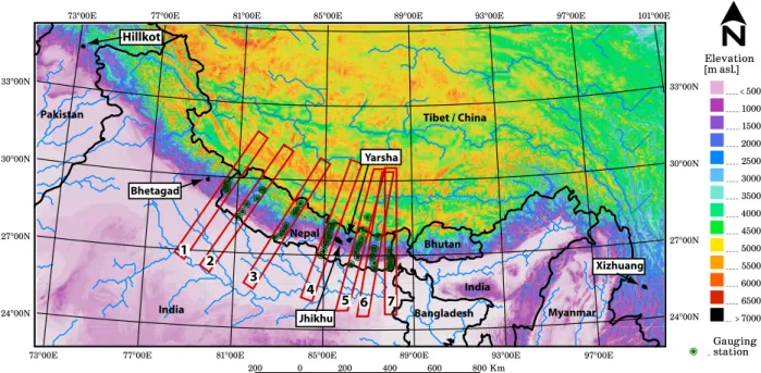
Figure 2. Topographic map of the Himalayan region. Arrows point at the location of the five PARDYP watersheds, where the data sets have been tested on a small scale for temporal accuracy. Red polygons outline the seven swath profiles across the Himalayan range, and green dots are the gauge station locations.

precision and high‐resolution global precipitation maps from satellite observations. The project is sponsored by Core Research for Evolutional ence and Technology (CREST) of the Japan Sci-ence and Technology Agency (JST), by Japan Aerospace Exploration Agency (JAXA) and the Precipitation Measuring Mission (PMM) Science Team. GSMaP data are a global data set (60°N/S), available since the end of November 2002 and is provided in almost real time (with a∼10 month data gap in 2007). The data have 0.1° (∼10 km) spatial resolution and 1 h temporal. The project aims to develop an advanced microwave radiometer rithm based on a deterministic rain‐retrieval algo-rithm and the production of precise high‐resolution global precipitation maps [Ushio et al., 2009; Kubota et al., 2007]. The data incorporate MWR measures from TRMM‐TMI, SSM/I, Advanced Microwave Scanning Radiometer–EOS on board of AQUA satellite (AMSR‐E), AMSU‐B and IR. Because of its high spatiotemporal resolution this data set is potentially the most interesting for ana-lyzing climatic influence on surface processes and the links between rainfall distribution and topogra-phy. Dinku et al. [2009] compared GSMaP MVK+ with several other satellite derived precipitation data sets and gauge stations over the whole of Colombia. They report that GSMaP MVK+ underestimates precipitation in mountains, where the topography is complex.

2.1.4. TRMM‐3B42

[11] The Tropical Rainfall Measuring Mission

(TRMM) is a joint collaboration between JAXA and the United States of America National Aero-nautics and Space Administration (NASA). TRMM‐ 3B42, is a global multisatellite precipitation analysis data set. It combines several instruments, has a 0.25° (∼30 km) spatial and 3 h temporal resolution, and is available within a global belt, 50°N/S latitude [Huffman et al., 2007; Kummerow et al., 2000]. Basically it is a set of MWR estimates from TRMM‐ TMI, SSM/I, AMSR‐E and AMSU‐B, whereas missing pixels are filled with IR observations com-piled by CPC [Huffman et al., 2007]. The data are corrected with the monthly field ratios between TRMM‐3B43 (monthly compiled version of 3B42) and gauge stations. TRMM‐3B42 has been applied successfully for measuring precipitation patterns in many studies on a global [Tian and Peters‐Lidard, 2010] and local scale [Kamal‐Heikman et al., 2007; Bookhagen and Strecker, 2008; Bookhagen, 2010]. However, underestimation in mountainous regions,

in particular with high snowfall contribution [Kamal‐ Heikman et al., 2007], has been reported.

2.1.5. TRMM‐2B31

[12] Bookhagen and Burbank [2006] have

devel-oped their own precipitation compilation from primary TRMM‐2B31 orbital data (not gridded). Despite a common platform and name, TRMM‐ 2B31 and TRMM‐3B42 data set do not use the same sensor (except for TMI). TRMM‐2B31 is principally derived from the active PR sensor, found only on board of the TRMM satellite [Bookhagen and Burbank, 2006]. Here TRMM‐ TMI is used to fill unobserved areas. TRMM‐2B31 data have a spatial resolution of 0.05° (∼4 km), one of the finest grid size available at the moment. However its temporal resolution is 1 month, aver-aged over several years. The PR sensor makes one or two snapshots of the Earth surface per day (depending on the latitude). Therefore, measure-ments are infrequent and have to be averaged over a long time span (here: 11 years, 1997–2007) to provide reliable rainfall data [Bookhagen and Burbank, 2006]. This data set has been success-fully applied for measuring precipitation patterns in the Andes [Bookhagen and Strecker, 2008] and the Himalayas [Bookhagen and Burbank, 2006, 2010].

2.2. Rain Gauge Data

[13] We compared precipitation estimates from

each product with ground measurements derived from the 55 rain gauge stations located in Nepal (54) and on the Tibetan Plateau (1): Figure 2 (see also Text S1). Most of the data are obtained from the Department of Hydrology and Meteorology Nepal DHM (∼30 years data, numbers 1–51, Text S1). Three high elevation stations (3560, 4260 and 5050 m above sea level (asl), numbers 53–55) in the Khumbu‐ Everest region are kindly provided by the Ev‐K2‐ CNR, Pyramid‐SHARE project, while the station for the Tibetan Plateau (number 52) comes from the LocClim FAO database (http://www.fao.org/nr/ climpag/pub/en0201_en.asp). We also compared the precipitation data sets with ground information from rain gauge stations in five watersheds located in Pakistan, India, Nepal (2) and Yunnan/China (Figure 2) maintained within the People and Resource Dynamics Project (PARDYP) program, realized by International Centre for Integrated Mountain Devel-opment (ICIMOD) between 1997 and 2006. Note that the 51 gauge stations provided by DHM have been used to generate the APHRODITE data set so there

is a dependency problem between APHRODITE and these gauge station data. They might have also served to calibrate any of the other data sets. However, this is not the case for all the precipitation gauge data of the five PARDYP watersheds, as well as the three Pyramid‐SHARE stations (53–55), which provide independent data that have not been used to generate or calibrate any of these data sets. We presume the uncertainties of all precipitation gauge measurements to be≤10%.

2.3. Bulk Validation of Data

[14] To give an overview of the bulk error of each

data set at the scale of Nepal, we compared each data set with all rain gauge stations on a monthly scale. For this purpose, we subtracted the monthly accumulated ground measurements of each station from the corresponding monthly sum of each data set and average the difference considering all the stations. This comparison was carried out consid-ering only the data for the years 2003 and 2004. Because some of the 51 DHM stations might have been used to calibrate or generate some of the pro-ducts (in particular APHRODITE), we also evaluate the bulk error by considering only the stations that have not been used in the calibration or generation

stations within the five PARDYP watersheds). Because gauge data are not always available for the same period, we sampled precipitation and rain gauge data for months of common availability between 1997 and 2006 and calculated then the monthly bulk error of each product.

2.4. Calculation of Basin‐Wide Precipitation in Five Selected Watersheds

[15] We compared the precipitation data sets with

ground information from rain gauge stations in the five watersheds maintained within the PARDYP program (Figure 2). The five relatively small watersheds (15–111 km2, Table 1) have been equipped with several measuring devices to obtain meteorological, hydrological and erosional param-eters. In each watershed, data are available for 4 to 12 rainfall stations (Table 1) for 5 to 10 years, providing a very good data set of ground truth information to calibrate remote sensing information [Andermann et al., 2010]. The station elevation distribution is homogeneous for Bhetagad, Jhikhu Khola and Yarsha Khola basin (Figure 3), whereas in Xizhuang basin a large part between 2200 and 3000 m asl is not covered by stations. The higher part of the Hillkot basin (elevation >1800 m asl) is not covered by rain gauge stations (Figure 3). In each catchment, we interpolated (nearest neighbor interpolation technique) the available gauge data to a mean basin‐wide value. The mean basin‐wide value was then extracted from each data set. Since TRMM‐2B31 data do not exist with high temporal resolution (daily nor monthly) it was not included in the comparison of products here.

2.5. Calculation of Precipitation Along Swath Profiles

[16] We compared the precipitation data sets during

the years of common availability of all data sets, 2003 and 2004 (Figure 1), along seven swath profiles perpendicular to the Himalayan front (Figure 2). Each swath profile is 60 km wide and 650 km long. Precipitation and elevation along one profile represent the average over the swath width of the profile. Topography information is derived from the Shuttle Radar Topographic Mission (SRTM) Version 4 (A. Javis et al., Hole‐filled seamless SRTM data V4, International Centre for Tropical Agriculture (CIAT), 2008, available from http://srtm.csi.cgiar.org) with a spatial resolution of

Figure 3. Hypsometric profiles of each PARDYP watershed with gauge station distribution. Gauge station elevation is plotted on the y axis as the respective cumu-lative normalized elevation fraction of each watershed. Area on the x axis represents the cumulative fraction of area within the watershed for each respective eleva-tion above mean sea level.

∼90 m. Along the profiles, precipitation totals were compiled annually as well as for monsoon (June to September) and for the nonmonsoon season (October–May).

3. Results

[17] We present the results of the evaluation of

precipitation data sets, first the bulk difference between fully independent and semi‐independent gauge data and precipitation data sets. Second, we present results within the five PARDY catchments, allowing us to test the temporal quality of data, from annual to daily scale. Last, we present results along the swath profiles perpendicular to the Himalayan chain and examine the spatial variations of data with regard to elevation.

3.1. Bulk Error and Comparison of Products

[18] The annual bulk comparison between

pro-ducts and fully independent gauge data (Pyramid‐ SHARE and PARDYP), which have not been used to generate nor calibrate any product, including APHRODITE shows that CPC‐RFE, TRMM3B42 and GSMaP underestimate rain gauge data up to 400 mm yr−1, while TRMM‐2B31 considerably overestimates (∼600 mm/yr) the independent data set (Figure 4a). Precipitation is mainly underestimated during monsoon season (CPC‐RFE 52 mm/yr, TRMM3B42 77 mm/yr, GSMaP 130 mm/yr), while APHRODITE (maximal 12 mm/yr) does not sig-nificantly differ from gauge data, whatever the sea-son considered. Because of its temporal resolution, TRMM‐2B31 cannot be compared to rain gauge Table 1. Overview of the Selected Five PARDYP Watershedsa

Name Region/Country Area (km2) Elevation Range (m asl) Catchment Orientation Number of Stations Literature Bhetagad Uttaranchal/India 24 1000–2000 north 5 Kothyari et al. [2004]

Hillkot Pakistan 15 1500–2700 southwest 4 unpublished

Jhikhu Khola Nepal 111 800–2200 southeast 11 Merz [2004]

Xizhuang Yunnan/China 34 1750–3100 east 8 Jianchu et al. [2005]

Yarsha Khola Nepal 53 1000–3000 southwest 12 Merz [2004]

a

Area is the drainage area, and range is the elevation minima and maxima. Number of stations indicates the number of available precipitation gauge stations which have been used to interpolate mean basin‐wide precipitation rates. See also Figure 2.

Figure 4. Monthly and annual bulk error plots of the compared precipitation data sets (APHRODITE, CPC‐RFE, GSMaP, TRMM‐3B31, and TRMM‐2B42). Errors represent the mean accumulated sum (monthly or annual) of pre-cipitation gauge data subtracted from the prepre-cipitation data set. (a) Bulk error derived from independent gauge sta-tions. (b) Bulk error for all 51 DHM stations in Nepal, which have been partially used to calibrate or generate the here evaluated data sets. Stations and data represent the 2 years 2003 and 2004 (1997–2007 in case of TRMM‐ 2B31). Because of its temporal resolution, TRMM‐2B31 was not included in the monthly evaluation.

be done considering the 51 rain gauge data from DHM as a reference (Figure 4b). However, these stations have been used to generate APHRODITE, and some stations may have been used to calibrate all the other products. Despite this possible depen-dency problem, CPC‐RFE, TRMM3B42 and GSMaP always show a significant underestimation of pre-cipitation whereas TRMM‐2B31 overestimates gauge data, but to a lesser degree than with independent data (328 mm/yr).

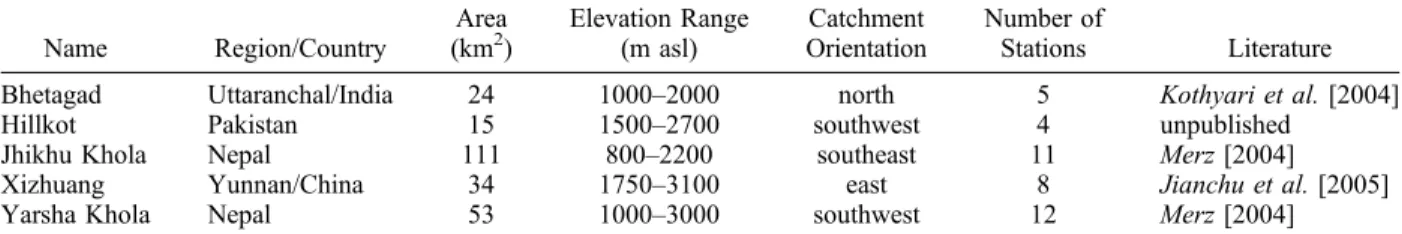
[19] Results from the bulk error analysis are also

reflected in the intercomparison of the data sets in map view (Figure 5). The available gridded pro-ducts show contrasting patterns of annual precipi-tation along the Himalayas. All products show high precipitation rates along the mountain chain, but with different amplitudes and patterns. Most pro-ducts show the westward decrease of precipitation already described by Bookhagen and Burbank [2006] as well as the two along‐strike rainfall peaks they also described. They are clearly expressed by TRMM‐ 2B31 because of the higher spatial resolution of this product. The comparison of the remote products with respect to APHRODITE shows that all products differ considerably in detail (Figures 5f, 5g, 5h, and 5i). It illustrates an overestimation of precipitation by TRMM‐2B31 with respect to APHRODTIE, possibly because APHRODITE cannot depict small‐ scale changes because of its moderate resolution (0.25°), but also because peak precipitation rates by TRMM‐2B31 are likely overestimated, as the authors acknowledge themselves [Bookhagen and Burbank, 2010]. When compared to APHRODITE, remotely sensed products CPC‐RFE, GSMaP and TRMM3B42 significantly underestimate precipita-tion in the eastern and central part of the Himalayas (Figures 5g, 5h, and 5i), while CPC‐RFE (Figure 5g) tends to overestimate precipitation in the Western part. All data sets show similar low precipitation rates (<0.5 m/yr) on the Tibetan Plateau and moderate ones (0.5–1 m/yr) in the Indian foreland.

3.2. Comparison of Data Within the Five PARDYP Watersheds

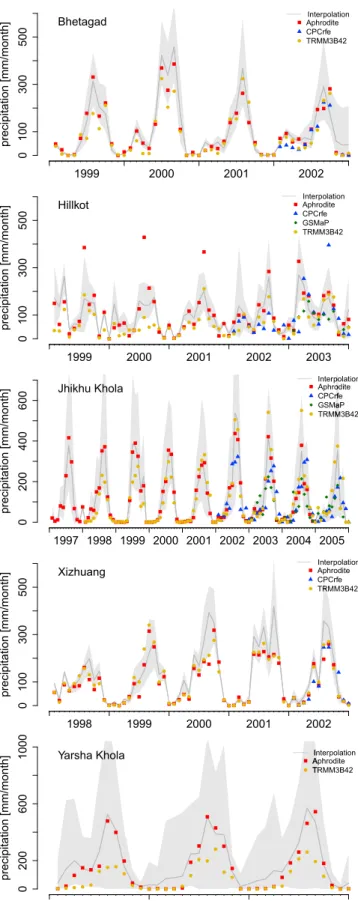
[20] Within the five PARDYP watersheds,

precip-itation estimates by APHRODITE and TRMM‐ 3B42 fit measurements derived from ground gauge stations, both at the monthly (Figures 6 and 7) and annual scales (Text S2). The correlation coefficient between monthly precipitations derived from gauge data and data sets is 0.87 for APHRODITE and

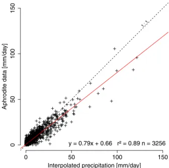
catchments all together (Figure 7). The best cor-relation is found in the Jhikhu Khola catchment with r2 of 0.98 (APHRODITE) and of 0.82 (TRMM‐3B42). APHRODITE always fit very well the monthly precipitation derived from gauge data (correlation coefficient between 0.83 and 0.98) except in the Hillkot catchment (Figure 6) where it gives higher estimates than the interpolated gauge data during monsoon season. This is likely the consequence of the lack of gauge stations at high elevations in this basin (Figure 3). Indeed, Bhatt and Nakamura [2005] and Barros et al. [2004] report strong ridge‐valley gradients on a basin scale in the Himalayan front. If we assume an orographic gradient, with lower precipitation in the valley bottom than close to the ridges, the absence of stations at high elevation in the Hillkot catch-ment will result in an underestimation of mean basin‐wide precipitation. Note that APHRODITE also correlates very well with precipitation derived from gauge stations at the daily scale in the Jhikhu Khola catchment (Figure 8). This correlation is not observed with the other data sets nor in the other basins. Monthly precipitation derived from TRMM‐ 3B42 usually correlates well with gauge data (cor-relation coefficient between 0.78 and 0.84; Text S2) except again in the Hillkot catchment, likely for the same reason as discussed above (correlation coeffi-cient of 0.52). Overall, CPC‐RFE and GSMaP data do not match the ground information at the annual and monthly scale (Figure 6).

[21] In contrast to observations made by Anders

et al. [2006] and Kamal‐Heikman et al. [2007], using remote precipitation measurements (TRMM/ PR and TRMM‐3b42), our annual precipitation estimates from APHRODITE or from interpolated rain gauge data exceed annual water discharge recorded at the catchment outlet of the five PARDYP watersheds. In Jhikhu Khola catchment for example, annual precipitation measured by APHRODITE, TRMM‐3B42 and by gauge stations (∼1400 mm/yr) is roughly 3.5 times as high as the annual specific discharge (∼400 mm/yr) recorded at the basin outlet [Merz, 2004]. As pointed out by Bookhagen and Burbank [2010] for the Himalayas, the hydrologic budget is only correct when evapotranspiration and snow and glacier melt processes are taken into account. High snowfall contribution on the Tibetan Plateau is difficult to detect by remote sensors and is shown to lead to considerable underestimation of basin‐wide water budgets [Kamal‐Heikman et al., 2007].

Figure 5. Mean annual precipitation distribution of the five tested precipitation data sets for their common availabil-ity (2003 and 2004, TRMM‐2B31 1997–2007): (a) APHRODITE, (b) TRMM‐2B31 [Bookhagen and Burbank, 2006], (c) CPC‐RFE, (d) GSMaP, and (e) TRMM‐3B42. Figures 5f–5i illustrate the differences between the data sets in respect to APHRODITE (APHRODITE‐ data set): (f) APHRODITE versus TRMM‐2B31, (g) APHRODITE versus CPC‐RFE2.0, (h) APHRODITE versus GSMaP, and (i) APHRODITE versus TRMM‐3B42.

Figure 6. Monthly mean basin‐wide precipitation rates from gridded precipitation data and basin‐wide interpolated rain gauge stations for the five watersheds. Gray shading represents the range of interpolated gauge data. The upper and lower limits of the range represent the minimal and maximal monthly sum of precipitation rates.

3.3. Comparison of Data Along the Seven Swath Profiles

[22] Evaluating the different data sets along swath

profiles has the advantage to investigate precipita-tion distribuprecipita-tion as a funcprecipita-tion of elevaprecipita-tion. Swath profiles show mean precipitation over the swath width and average over local variations. Therefore, gridded data sets with the same resolution (e.g., TRMM‐3B42 and APHRODITE) should match quantitatively. This is however not the case in our results (Figure 9).

[23] While the middle hills and the foreland are

easily accessible, the High Himalayas are only sparsely covered with stations and the station ele-vation might not reflect the surroundings [Bhatt and Nakamura, 2005]. However, most existing rain gauge data indicate high precipitation rates in the Lesser Himalaya and a decrease at higher ele-vation, in the Higher Himalayas and on the Tibetan Plateau. Along most profiles (Figure 9 and Text S3), gauge data consequently document the orographic effect across the Himalayas, despite possible pro-blems of point data vs. spatial data. Due to inac-cessibility, gauge stations are generally situated in valleys, especially within the high Himalayan range (Text S3). Note that most stations used here are situated at mean swath elevation in the transition between the Indian Lowlands and the mountain front (e.g., stations 16, 17, 18, 19, and 20 along profile 3: Figure 9a and Text S3), whereas stations

in the high mountain front are situated at minimum elevation of the swath profile (e.g., stations 12, 13, 14, and 15 along profile 3: Figure 9a and Text S3). Therefore, along profile 3 it is not clear if the decreasing trend defined by stations 18 and 14 is due to elevation or stations positioning. In contrast, thanks to the three Pyramid‐SHARE stations (numbers 53–55), nearly all stations in profile 5 (Figure 9d) are situated close to mean elevation (Text S3). Here, the strong decrease in precipitation rates between stations 31 and 55, above 3000 m asl is likely the consequence of the orographic effects. Locally, the annual difference between two neigh-boring stations is remarkable, e.g., between stations 46 and 48 (profile 7, Text S3) or between stations 38 and 44 (profile 6, Figure 9g). In both cases the stations are almost at the same latitude but at dif-ferent elevation, so they likely record difdif-ferent local annual precipitation variations linked to orography.

[24] For the data sets evaluated here, all seven

swath profiles (Figure 9 and Text S3) illustrate the orographic effect of the Himalayan chain, on annual scale as well as during monsoon season (May–October). Depending on the data set, the amplitude of the orographically induced rainfall peak is more or less pronounced. The orographic influence during nonmonsoon season is much weaker, as already observed by Bookhagen and Burbank [2010]. Overall, all data sets are more or less consistent during nonmonsoon season.

Figure 7. Correlation between monthly basin‐wide precipitation rates from gridded data and basin‐wide interpolation from station data. Data from all five water-sheds is plotted here.

Figure 8. Daily correlation (Jhikhu Khola, Nepal) between APHRODITE data and basin‐wide mean inter-polated precipitation rates.

Figure 9. Precipitation swath profiles (a, b, and c) 3, (d, e, and f) 5, and (g, h, and i) 6 (further profiles are given in Text S3). Mean annual precipitation is give Figures 9a, 9d, and 9g for each precipitation data set and swath profile, plotted against elevation from north to south. Shaded curves represent maxim um, minimum, and mean values along each swath profile. The gridded data are for the years of common availability (2003 and 2004), while TRMM ‐2B31 [Bookhagen and Burbank 2006] is for a 10 year time span (1997 –2007). Gauge data are plotted as mean values for both time spans. Error bars show the long ‐term (∼ 30 years) maxima minima. Figures 9b, 9e, and 9h represent the monsoon season (June –September) only. Figures 9c, 9f, and 9i represent the nonmonsoon season (October –May).

[25] Along the Himalayan front, annual

precipita-tion estimates at a given locaprecipita-tion along the profiles are always maximum for TRMM‐2B31 data and minimum for GSMaP, the difference being often as large as two‐ to threefold (Figures 9a, 9d, and 9g). Between these two extreme data sets, APHRODITE usually shows higher estimates than TRMM‐3B42 and CPC‐RFE data, except for profiles 1 and 2 (Text S3) where the latter delivers the highest values. The three Pyramid‐SHARE project stations (independent to APHRODITE) fit very well with the APHRODITE data, on an annual as well as a seasonal scale (Figures 9d–9f). A striking feature is the large difference between TRMM‐2B31 data set and all the other data sets when considering mean and maximum values, as well as the high frequency spatial variations of precipitations documented. This is a direct consequence of the high spatial resolution of this data set. Overall, most of the gauge stations usually plot near the mean value of the TRMM‐2B31 product, except for some local examples (e.g., stations 27 and 29 in profiles 4; stations 12 and 13 in profile 3; stations 31 and 34 in profile 5; stations 38, 39 and 41 in profile 6: see Figure 9 and Text S3). The extreme values of the TRMM‐2B31 product always exceed gauge values (e.g., extremely high precipitation values (>7000 mm/yr) for few pixels on profile 3, Figure 9a), as already noticed by Bookhagen and Burbank [2010] and Anders et al. [2006]. These extreme values likely overestimate real precipitation rates. Note that Bookhagen and Burbank [2006] used a network of rainfall stations to calibrate their TRMM‐ 2B31 data; however, most of the stations we used here have not been used in their work. In general the swath profiles reflect the findings of the bulk error estimation (Figure 4).

[26] Bookhagen and Burbank [2010, 2006]

demon-strated that precipitation profiles across the Hima-layas mimic the topography. When the topography steadily increases from the Indian Lowland to the Tibetan Plateau, rainfall distribution is character-ized by a single high peak of rainfall at elevation ∼0.9 km. Conversely, for a two‐stepped increase of topography, rainfall distribution shows two peaks of lower amplitude at ∼0.9 km and 2.1 km (e.g., Figures 5b and 9g). This bimodal distribution of rainfall is visible in most of the TRMM‐2B31 pro-files we show here (e.g., propro-files 1, 4, and 6). This particular distribution is also well depicted by the APHRODITE product in most cases (e.g., profiles 1, 4, and 6) but with a lower amplitude. However, this is usually not depicted by the other products, except in profile 1 (Text S3). Overall, all the products show

the increase of precipitation rates at the front of the Himalayas. TRMM‐3B42, GSMaP and CPC‐RFE, however, do not describe correctly the precipitation distribution at elevations higher than 1 km. This result highlights the difficulty of remote sensing techniques to capture precipitation in areas with strong oro-graphic effects. The direct comparison of TRMM‐ 2B31 and TRMM‐3B42 in the Andes already shows that TRMM‐3B42 cannot detect the local orographic precipitation maxima, due to its moderate spatial resolution [Bookhagen and Strecker, 2008].

4. Discussion and Conclusion

[27] We show that existing gridded precipitation

data sets as well as published sources [Bookhagen and Burbank, 2006] display large differences along the Himalayan orographic front. With the exception of CPC‐RFE, all measurements corre-spond in low‐relief landscapes (Indian Lowlands, Tibetan Plateau) and during nonmonsoon season. On the basis of comparison with independent ground observations (Figure 4a) we show that most remote products underestimate precipitation during monsoon season at the annual and monthly scale whereas TRMM‐2B31 [Bookhagen and Burbank, 2006] overestimates precipitation at the annual scale. These problems of precipitation estimation are likely due to remote techniques and calibration procedures. They do not concern APHRODITE data, a product processed from gauge stations, which gives the best precipitation estimates when compared to independent ground observations (Figure 4a). However, the lack of stations at high elevation limits the accuracy of this data set.

[28] Most of the rain gauges used to calibrate CPC‐

RFE, GSMaP and TRMM‐3B42 data are derived from the GTS network with reportedly poor spatial coverage in the Himalayas [Yatagai and Kawamoto, 2008], which might explain the underestimation of precipitation during monsoon season. Additionally, Yatagai and Kawamoto [2008] report that the GTS database includes erroneous entries in the Himala-yan region, where 0 mm precipitation values were reported instead of missing values, thus resulting in underestimating precipitation. In the case of APH-RODITE, up to 4.5 times as many stations as GTS were considered for interpolation and erroneous gauge data sets are excluded if other information existed for the interpolation space [Yatagai and Kawamoto, 2008]. Many difficulties in the estima-tion of precipitaestima-tion from space may also arise from remote techniques themselves. Remote sensors can-not determine accurately snowfall which is the major

(>5000 m asl: [Putkonen, 2004]) and on the Tibetan Plateau. Data sets depending on IR observations are primarily sensitive to cloud‐top temperature, whose calibration for estimating precipitation is a main source of uncertainty [Huffman et al., 2007]. Finally, diurnal variations and the likeliness of the satellites to miss rainfall events, may participate to the discrep-ancy between the remote measurements. CPC‐RFE, GSMaP and TRMM‐3B42 are principally derived from MVR sensors, which have an irregular return interval and therefore, likely miss precipitation events [Huffman et al., 2007].

[29] Our study also highlights some of the

diffi-culties in evaluating remote precipitation products using rainfall gauge data. In the Himalayas, pre-cipitation varies according to a wide range of spatial scales, from small‐scale ridge‐valley gradients [Barros et al., 2004; Bhatt and Nakamura, 2005; Anders et al., 2006; Craddock et al., 2007] to large‐scale orographic effects over the whole mountain [Anders et al., 2006; Bookhagen and Burbank, 2006]. Ide-ally, the validation of any remote sensed product from gauge stations is only possible if the resolution of the products is sufficient to take into account the scale of spatial variability of precipitation. Hence, the coarse resolution of all products (Figure 1) introduce an inescapable problem in the validation procedure. For example, gauge stations in valleys within the High Himalayas (e.g., profile 3; see Text S3) likely introduce a bias in the reference value of precipitation they provide. We show that several stations, covering full elevation range, are necessary to represent the climatic situation cor-rectly and to validate remotely sensed products. We also show that basin‐wide precipitation measure-ment deduced from gauge data are significantly altered if elevation is not sufficiently covered by gauge stations (Hillkot watershed, Figure 6). The current gauge network within the High Himalayas is generally not sufficient to characterize orographic precipitation phenomena correctly.

[30] Along the Himalayan range, several

precipi-tation products are of potential interest depending on the problem addressed. TRMM‐2B31 is a good product when one wants to investigate rainfall patterns. This is of significant interest for example to understand the topographic influence on rain distribution. The use of this product is however, limited by its temporal resolution, which is not adequate to investigate, for example, event‐scale processes. As also observed by Bookhagen and Burbank [2006], the rainfall peaks of TRMM‐

overestimated. TRMM‐2B31 describes correctly the large‐scale orographic rainfall distribution along the Himalayan front. This distribution is poorly depicted by all other data sets based on remote sensing techniques. As in the work by Tian and Peters‐Lidard [2010], our study shows that sensor algorithms for mountainous regions, where terrain changes on short distances and orography influ-ences precipitation, must be improved.

[31] As observed in the five small watersheds

studied here, APHRODITE (and to a lesser extent TRMM‐3B42) deliver good temporal variability, both on annual and monthly scale. In some cases, for example in the Jhikhu Khola catchment, which is located in the lower middle mountains with a low relief (∼1400 m), even daily precipitation estimates by APHRODITE are representative (Figure 8). Because of its long availability (>30 years), coupled with its good temporal resolution, the APHRODITE product is appropriate to track above‐threshold events driven by precipitation (e.g., landslides thresholds [Gabet et al., 2004; Dahal and Hasegawa, 2008]) as well as for hydrological budget and dis-charge analysis. It can be applied for hydrolog-ical budget and discharge analysis of large basins (>2000 km2∼ 2 pixels). If higher temporal resolu-tion than APHRODITE is needed, then the TRMM‐ 3B42 data, with its 3‐hourly resolution, could also be exploited for relative analysis, even if not tested here. Accurate precipitation data in an active moun-tain belt such as the Himalayas are essential for a real understanding of the potential couplings between climate, erosion and tectonics processes as well as for hazard mitigation.

Acknowledgments

[32] We would like to thank the German academic exchange service DAAD and the French German university DFH for funding the Ph.D. thesis of C. Andermann. Pyramid Ev‐K2‐ CNR–SHARE project for meteorological data. We would like to thank Madhav Dhakal and Isabelle Providolli from ICIMOD Kathmandu for their outstanding support, Jianchi Xu and Ma Xing for readily sharing information on Xizhuang watershed, as well as B. P. Kothyari from GBPIHED India for providing data on Bhetagad watershed. Many thanks go also to Bodo Bookhagen for providing us with a mean annual data set of TRMM‐2B31. We would like to thank Jagadish Karmacharya from DHM Nepal for his great support to select and obtain gauge data. We thank Alain Crave for helpful discussions and Guillaume Dupont‐Nivet for proofreading. We would also like to thank two anonymous reviewers and the Editor of G‐cubed, Louis Derry, whose comments and suggestions have considerably improved this manuscript.

References

Andermann, C., S. Bonnet, and R. Gloaguen (2010), Erosion in the Himalayas on catchment scale. Integrative remote sensing assessment, in Geoscience and Remote Sensing Symposium, 2009 IEEE International, IGARSS 2009, vol. 3, IEEE, Washington, D. C., doi:10.1109/IGARSS.2009.5417866. Anders, A. M., G. H. Roe, B. Hallet, D. R. Montgomery, N. J.

Finnegan, and J. Putkonen (2006), Spatial patterns of precip-itation and topography in the Himalaya, GSA Spec. Pap., 398, 39–53, doi:10.1130/2006.2398(03).

Anders, A. M., G. H. Roe, D. R. Montgomery, and B. Hallet (2008), Influence of precipitation phase on the form of mountain ranges, Geology, 36(6), 479–482, doi:10.1130/ G24821A.1.

Barros, A. P., G. Kim, E. Williams, and S. W. Nesbitt (2004), Probing orographic controls in the Himalayas during the monsoon using satellite imagery, Nat. Hazards Earth Syst. Sci., 4(1), 29–51, doi:10.5194/nhess-4-29-2004.

Barros, A. P., S. Chiao, T. J. Lang, D. Burbank, and J. Putkonen (2006), From weather to climate: Seasonal and interannual variability of storms and implications for erosion processes in the Himalaya, GSA Spec. Pap., 398, 17–38, doi:10.1130/ S2006.2398(02).

Bhatt, B. C., and K. Nakamura (2005), Characteristics of mon-soon rainfall around the Himalayas revealed by TRMM pre-cipitation radar, Mon. Weather Rev., 133(1), 149–165, doi:10.1175/MWR-2846.1.

Bonnet, S. (2009), Shrinking and splitting of drainage basins in orogenic landscapes from the migration of the main drainage divide, Nat. Geosci., 2(11), 766–771, doi:10.1038/ngeo666. Bonnet, S., and A. Crave (2003), Landscape response to climate change: Insights from experimental modeling and implications for tectonic versus climatic uplift of topography, Geology, 31(2), 123–126, doi:10.1130/0091-7613(2003)031< 0123:LRTCCI>2.0.CO;2.

Bookhagen, B. (2010), Appearance of extreme monsoonal rainfall events and their impact on erosion in the Himalaya, Geomatics Nat. Hazards Risk, 1(1), 37–50, doi:10.1080/ 19475701003625737.

Bookhagen, B., and D. W. Burbank (2006), Topography, relief, and TRMM‐derived rainfall variations along the Himalaya, Geophys. Res. Lett., 33, L08405, doi:10.1029/ 2006GL026037.

Bookhagen, B., and D. W. Burbank (2010), Toward a com-plete Himalayan hydrological budget: Spatiotemporal distri-bution of snowmelt and rainfall and their impact on river discharge, J. Geophys. Res., 115, F03019, doi:10.1029/ 2009JF001426.

Bookhagen, B., and M. R. Strecker (2008), Orographic bar-riers, high‐resolution TRMM rainfall, and relief variations along the eastern Andes, Geophys. Res. Lett., 35, L06403, doi:10.1029/2007GL032011.

Craddock, W. H., D. W. Burbank, B. Bookhagen, and E. J. Gabet (2007), Bedrock channel geometry along an oro-graphic rainfall gradient in the upper Marsyandi River valley i n c e n t r a l N e p a l , J . G e o p h y s . R e s ., 1 1 2 , F 0 3 0 0 7 , doi:10.1029/2006JF000589.

Dahal, R. K., and S. Hasegawa (2008), Representative rainfall thresholds for landslides in the Nepal Himalaya, Geomorphol-ogy, 100(3–4), 429–443, doi:10.1016/j.geomorph.2008.01.014. Dinku, T., F. Ruiz, S. J. Connor, and P. Ceccato (2009), Val-idation and intercomparison of satellite rainfall estimates over Colombia, J. Appl. Meteorol. Climatol., 49(5), 1004–1014, doi:10.1175/2009JAMC2260.1.

Gabet, E. J., D. W. Burbank, J. K. Putkonen, B. A. Pratt‐Sitaula, and T. Ojha (2004), Rainfall thresholds for landsliding in the Himalayas of Nepal, Geomorphology, 63(3–4), 131–143, doi:10.1016/j.geomorph.2004.03.011.

Huffman, G. J., R. F. Adler, D. T. Bolvin, G. Gu, E. J. Nelkin, K. P. Bowman, Y. Hong, E. F. Stocker, and D. B. Wolff (2007), The TRMM Multisatellite Precipitation Analysis (TMPA): Quasi‐global, multiyear, combined‐sensor preci-pitation estimates at fine scales, J. Hydrometeorol., 8(1), 38–55, doi:10.1175/JHM560.1.

Istanbulluoglu, E., and R. L. Bras (2006), On the dynamics of soil moisture, vegetation, and erosion: Implications of climate variability and change, Water Resour. Res., 42, W06418, doi:10.1029/2005WR004113.

Jianchu, X., A. Xihui, and D. Xiqing (2005), Exploring the spatial and temporal dynamics of land use in Xizhuang watershed of Yunnan, southwest China, Int. J. Appl. Earth Obs. Geoinf., 7(4), 299–309, doi:10.1016/j.jag.2005.06.008. Kamal‐Heikman, S., L. A. Derry, J. R. Stedinger, and C. C. Duncan (2007), A simple predictive tool for lower Brahma-putra River basin monsoon flooding, Earth Interact., 11(21), 1–11, doi:10.1175/EI226.1.

Kothyari, B. P., P. K. Verma, B. K. Joshi, and U. C. Kothyari (2004), Rainfall‐runoff‐soil and nutrient loss relationships for plot size areas of Bhetagad watershed in central Hima-laya, India, J. Hydrol., 293(1–4), 137–150, doi:10.1016/j. jhydrol.2004.01.011.

Kubota, T., et al. (2007), Global Precipitation map using satellite‐ borne microwave radiometers by the GSMaP project: Produc-tion and validaProduc-tion, IEEE Trans. Geosci. Remote Sens., 45(7), 2259–2275, doi:10.1109/TGRS.2007.895337.

Kummerow, C., W. Barnes, T. Kozu, J. Shiue, and J. Simpson (1998), The Tropical Rainfall Measuring Mission (TRMM) sensor package, J. Atmos. Oceanic Technol., 15(3), 809–817, doi:10.1175/1520-0426(1998)015<0809:TTRMMT>2.0. CO;2.

Kummerow, C., et al. (2000), The status of the Tropical Rain-fall Measuring Mission (TRMM) after two years in orbit, J. Appl. Meteorol., 39(12), 1965–1982, doi:10.1175/1520-0450(2001)040<1965:TSOTTR>2.0.CO;2.

Merz, J. (2004), Water balances, floods and sediment transport in the Hindu Kush‐Himalayas, Ph.D. thesis, Inst. of Geogr., Univ. of Bern, Bern, Switzerland.

Nesbitt, S. W., and A. M. Anders (2009), Very high resolution precipitation climatologies from the Tropical Rainfall Mea-suring Mission precipitation radar, Geophys. Res. Lett., 36, L15815, doi:10.1029/2009GL038026.

Putkonen, J. (2004), Continuous snow and rain data at 500 to 4400 m altitude near Annapurna, Nepal, 1999–2001, Arct. Antarct. Alp. Res., 36(2), 244–248, doi:10.1657/1523-0430(2004)036[0244:CSARDA]2.0.CO;2.

Reiners, P. W., T. A. Ehlers, S. G. Mitchell, and D. R. Montgomery (2003), Coupled spatial variations in precipitation and long‐term erosion rates across the Washington Cascades, Nature, 426(6967), 645–647, doi:10.1038/nature02111. Roe, G. H. (2005), Orographic precipitation, Ann. Rev. Earth

Planet. Sci., 33(1), 645–671, doi:10.1146/annurev.earth.33. 092203.122541.

Roe, G. H., D. R. Montgomery, and B. Hallet (2003), Oro-graphic precipitation and the relief of mountain ranges, J. Geophys. Res., 108(B6), 2315, doi:10.1029/2001JB001521. Shrestha, M., G. Artan, S. Bajracharya, and R. Sharma (2008), Using satellite‐based rainfall estimates for streamflow mod-elling: Bagmati Basin, J. Flood Risk Manage., 1(2), 89–99, doi:10.1111/j.1753-318X.2008.00011.x.

uncertainties in satellite‐based precipitation measurements, Geophys. Res. Lett., 37, L24407, doi:10.1029/2010GL046008. Tucker, G. E., and R. Slingerland (1997), Drainage basin responses to climate change, Water Resour. Res., 33(8), 2031–2047, doi:10.1029/97WR00409.

Tustison, B., D. Harris, and E. Foufoula‐Georgiou (2001), Scale issues in verification of precipitation forecasts, J. Geophys. Res., 106(D11), 11,775–11,784, doi:10.1029/2001JD900066. Ushio, T., K. Sasashige, T. Kubota, S. Shige, K. Okamoto, K. Aonashi, T. Inoue, N. Takahashi, and T. Iguchi (2009), A Kalman filter approach to the Global Satellite Mapping of Precipitation (GSMaP) from combined passive microwave and infrared radiometric data, J. Meteorol. Soc. Jpn., 87A(9), 3084–3097, doi:10.2151/jmsj.87A.137.

Vicente, G. A., J. C. Davenport, and R. A. Scofield (2002), The role of orographic and parallax corrections on real time high resolution satellite rainfall rate distribution, Int. J. Remote Sens., 23(2), 221–230, doi:10.1080/01431160010006935. Whipple, K. X. (2009), The influence of climate on the tectonic

evolution of mountain belts, Nat. Geosci., 2(2), 97–104, doi:10.1038/ngeo413.

Whipple, K. X., and B. J. Meade (2006), Orogen response to changes in climatic and tectonic forcing, Earth Planet. Sci. Lett., 243(1–2), 218–228, doi:10.1016/j.epsl.2005.12.022.

erosion on the structure of mountain belts, J. Geophys. Res., 104(B12), 28,957–28,981, doi:10.1029/1999JB900248. Wulf, H., B. Bookhagen, and D. Scherler (2010), Seasonal pre-cipitation gradients and their impact on fluvial sediment flux in the northwest Himalaya, Geomorphology, 118(1–2), 13–21, doi:10.1016/j.geomorph.2009.12.003.

Xie, P., Y. Yarosh, T. Love, J. E. Janowiak, and P. A. Arkin (2002), A real‐time daily precipitation analysis over South Asia, paper presented at the 16th Conference of Hydrology, Am. Meteorol. Soc., Orlando, Fla., 12–17 Jan. (Available at http://www.cpc.ncep.noaa.gov/products/fews/sasia_r fe.pdf) Xie, P., M. Chen, S. Yang, A. Yatagai, T. Hayasaka, Y. Fukushima,

and C. Liu (2007), A gauge‐based analysis of daily precipita-tion over East Asia, J. Hydrometeorol., 8(3), 607–626, doi:10.1175/JHM583.1.

Yatagai, A., and H. Kawamoto (2008), Quantitative estimation of orographic precipitation over the Himalayas by using TRMM/PR and a dense network of rain gauges, in Proc. SPIE, 7148‐11, doi:10.1117/12.811943.

Yatagai, A., O. Arakawa, K. Kamiguchi, H. Kawamoto, M. I. Nodzu, and A. Hamada (2009), A 44‐year daily gridded pre-cipitation data set for Asia based on a dense network of rain gauges, SOLA, 5, 137–140, doi:10.2151/sola.2009-035.