The indication of Martian gully formation processes by slope–area analysis

HAL Id: insu-02276823

https://hal-insu.archives-ouvertes.fr/insu-02276823

HAL is a multi-disciplinary open access

archive for the deposit and dissemination of sci-entific research documents, whether they are pub-lished or not. The documents may come from teaching and research institutions in France or abroad, or from public or private research centers.

L’archive ouverte pluridisciplinaire HAL, est destinée au dépôt et à la diffusion de documents scientifiques de niveau recherche, publiés ou non, émanant des établissements d’enseignement et de recherche français ou étrangers, des laboratoires publics ou privés.

The indication of Martian gully formation processes by

slope–area analysis

Susan Conway, Matthew Balme, John Murray, Martin Towner, Chris Okubo,

Peter Grindrod

To cite this version:

Susan Conway, Matthew Balme, John Murray, Martin Towner, Chris Okubo, et al.. The indication of Martian gully formation processes by slope–area analysis. The Geological Society, London, Special Publications, Geological Society of London, 2011, 356 (1), pp.171-201. �10.1144/SP356.10�. �insu-02276823�

1

The indication of martian gully formation processes by slope-area analysis.

1

*Susan J. Conway 2

Work done at: Earth and Environmental Sciences, Open University, Walton Hall, Milton

3

Keynes MK7 6AA UK tel:+44 (0)1908 659777 fax:+44 (0)1908 655151 4

Now at: Laboratoire de planétologie et géodynamique, CNRS UMR 6112, Université de

5

Nantes, 2 rue de la Houssinière, BP 92208, 44322 Nantes cedex, France tel : +33 (0)251 6 125570 Susan.Conway@univ-nantes.fr 7 8 Matthew R. Balme 9

Earth and Environmental Sciences, Open University, Walton Hall, Milton Keynes MK7 6AA 10

UK tel:+44 (0)1908 659776 fax:+44 (0)1908 655151 m.r.balme@open.ac.uk 11

12

John B. Murray

13

Earth and Environmental Sciences, Open University, Walton Hall, Milton Keynes MK7 6AA 14

UK tel:+44 (0)1908 659776 fax:+44 (0)1908 655151 j.b.murray@open.ac.uk 15

16

Martin C. Towner

17

Impacts and Astromaterials Research Centre, Department of Earth Science and Engineering, 18

Imperial College London, SW7 2AZ, UK. tel:+44 (0)20759 47326 fax:+44 (0) 20 7594 7444 19 m.towner@imperial.ac.uk 20 21 Chris H. Okubo 22

Astrogeology Science Center, U.S. Geological Survey 2255 N. Gemini Dr. 23

Flagstaff, AZ 86001, USA tel:+1 (928) 556-7015 fax:+1 (928) 556-7014 cokubo@usgs.gov 24

25

Peter M. Grindrod

26

Department of Earth Sciences, University College London, Gower Street, London WC1E 27 6BT UK tel:+44 (0)20 7679 7986 28 p.grindrod@ucl.ac.uk 29 30

*Corresponding author (e-mail: s.j.conway@open.ac.uk) 31

2 33 Number of words: 12 624 34 Number of References: 180 35 Number of Tables: 2 36 Number of Figures: 11 37

The styles for each heading level: 38

Heading 1

Heading 2

Running title: Martian gully formation processes. 42

3

Abstract

44

The formation process of recent gullies on Mars is currently under debate. This study aims to 45

discriminate between the proposed formation processes: pure water flow, debris flow and dry 46

mass wasting, through the application of geomorphological indices commonly used in 47

terrestrial geomorphology. We used high resolution digital elevation models of Earth and 48

Mars to evaluate the drainage characteristics of small slope sections. We have used the data 49

from Earth to validate the hillslope, debris flow and alluvial process domains previously 50

found for large fluvial catchments on Earth, and have applied these domains to gullied and 51

ungullied slopes on Mars. In accordance with other studies our results indicate that debris 52

flow is one of the main processes forming the martian gullies that we studied. The source of 53

the water is predominantly distributed surface melting, not an underground aquifer. We also 54

present evidence that other processes may have shaped martian crater slopes, such as ice 55

assisted creep and solifluction, in agreement with proposed recent martian glacial and 56

periglacial climate. Our results suggest that, within impact craters, different processes are 57

acting on differently oriented slopes, but further work is needed to investigate the potential 58

link between these observations and changes in martian climate. 59

60 61

4 Martian “gully” landforms were first described by Malin & Edgett (2000) and defined as 62

features that have an alcove, channel and debris apron with the general appearance of gullies 63

carved by water. Within this definition gullies have a wide range of morphologies (Fig. 1) 64

and they are found in abundance on steep slopes at mid latitudes in both hemispheres on Mars 65

(e.g., Heldmann & Mellon 2004; Heldmann et al. 2007). They are interpreted to be 66

geologically young features because of the pristine appearance and paucity of superposed 67

impact craters. Recent work has suggested that some gullies have been active in the last 68

3 - 1.25 Ma (Reiss et al. 2004; Schon et al. 2009). Malin et al. (2006) observed new, high-69

albedo, dendritic deposits (named light-toned deposits) located along the paths of some 70

gullies, and which formed between subsequent images taken by the Mars Orbiter Camera 71

(MOC). These light-toned deposits have been attributed to either dry mass wasting (Pelletier 72

et al. 2008; Kolb et al. 2010), or debris flow (Heldmann et al. 2010), involving up to 50 % 73

water (Iverson 1997). However, the origins of these deposits are still under debate and it is 74

not clear whether they are related to the formation processes of the gullies, or whether they 75

are formed by a secondary process. 76

The formation process for martian gullies in general is also still under debate. Three 77

main candidates exist: (1) aquifer outflow, (2) surface melting, or (3) dry granular flow. In 78

the aquifer model the water is either released from a near surface confined aquifer (Malin & 79

Edgett 2000; Heldmann et al. 2005) or brought up from depth by cryovolcanic processes 80

(Gaidos 2001). The main criticism of the aquifer based models is their failure to explain the 81

location of some gullies on isolated hills, impact crater central peaks, mesas and sand dunes. 82

Melting of near surface ground ice or surface ice has been proposed for the formation of 83

gullies under recent obliquity excursions (Costard et al. 2002). There is growing support for 84

this model with the most compelling arguments being: (1) the majority of gullies exists at 85

mid-latitudes, (2) the dominance of pole-facing gullies (Balme et al. 2006; Dickson et al. 86

5 2007; Kneissl et al. 2009) and, (3) observations of coincidence with sites of seasonal surface 87

ice accumulation (Dickson & Head 2009). Granular flow has been suggested as either 88

unassisted (Treiman 2003; Shinbrot et al. 2004), or carbon dioxide assisted flow 89

(Musselwhite et al. 2001). The main criticism of the granular flow model is that it fails to 90

replicate some commonly observed features of gullies, in particular channel sinuosity and 91

complex tributary and distributary systems (McEwen et al. 2007). 92

There is also debate about the type of fluid involved: pure water, or brine. Whilst 93

pure water is not stable under the current surface environment on Mars, it can persist in a 94

metastable form (Hecht 2002), although its flow behaviour may be substantially different to 95

water on Earth (Conway et al. 2010a). Brines are a likely product of water sourced from 96

underground and, moreover, the presence of some common geological compounds can 97

substantially depress the freezing point of water (e.g., Chevrier & Altheide 2008). Brines are 98

less likely in a surface melting scenario, because water ice condensed from the atmosphere 99

will have had less opportunity to dissolve salts than an underground water body. Both pure 100

water and brine can support very high concentrations of entrained sediment, and form a flow 101

commonly termed a “debris flow”. Debris flow is an attractive candidate process for forming 102

gullies, because large amounts of erosion and deposition can be brought about with only 10 to 103

50 % water content (Iverson 1997). Several authors have proposed debris flow as a potential 104

gully-forming mechanism on Mars due to the supply of loose sediment combined with the 105

steep slopes on which gullies are found (e.g., Malin & Edgett 2000; Balme et al. 2006). The 106

inclusion of debris might also limit evaporation and freezing of the water within the flow. 107

Debris flows on Earth are commonly triggered by sudden and intense or prolonged rainfall, 108

(e.g., Ben David-Novak et al. 2004; Decaulne & Sæmundsson 2007; Godt & Coe 2007; 109

Crosta & Frattini 2008; Morton et al. 2008) which is not a possible mechanism on Mars 110

under recent climate. However, debris flows can also be triggered by snowmelt, or melting 111

6 permafrost (Harris & Gustafson 1993; Decaulne et al. 2005). As noted by Lanza et al. (2010) 112

infiltration rates on Mars are likely to exceed the low discharge rates produced by a surface 113

melting source. Hence, overland flow is unlikely, unless there is a shallow impermeable 114

barrier, such as near-surface permafrost, or frozen layer formed at the base of the water flow 115

on contact with a cold substrate (Conway et al. 2010a). The dominance of infiltration satisfies 116

the conditions for debris flow triggering, sediment saturation and elevated pore pressures. 117

The lack of vegetation and the associated lower cohesion of the martian soil, compared to 118

Earth, potentially means that debris flows can be triggered on much lower slope gradients 119

than they are on Earth. 120

Gullies formed by dilute-water flow and debris flow on Earth can be visually very 121

similar to each other, and the basic structure of gullies can be formed by dry granular flow 122

(Mangeney et al. 2007). In many geomorphological problems, convergence of visual form 123

means that using images alone can make it very difficult to determine process. The ongoing 124

debate regarding the formation mechanisms of gullies on Mars is a prime example of this. For 125

example some workers have dismissed debris flow as a mechanism for forming martian 126

gullies, because they have not observed the levées that are one of the diagnostic features of 127

debris flow (e.g., Innes 1983). However, the ability to identify levées depends on viewing 128

geometry and sun angle; metre sized levées are often not visible on 25 cm/pixel air photos of 129

Earth. It is also possible that a combination of the lower gravity and different sediment type 130

on Mars means that the levées might be small compared to those on Earth. 131

The amount of water required to carve channels and transport and deposit sediment 132

differs substantially between debris flow, water or brine flow (termed “alluvial” throughout 133

the rest of this paper) and granular flow. Determining the amount of water available at the 134

martian surface is important for questions of martian climate, hydrology and the study of 135

potential martian habitats. Hence, an accurate determination of active processes is needed that 136

7 in turn can constrain the quantity of fluid required to form gullies. Quantitative 137

geomorphological study can provide the tools to discriminate between these three processes. 138

The recent availability of high resolution digital elevation models (DEMs) of Mars has 139

opened up the possibility of using quantitative geomorphic methods that have, until now, 140

been restricted to analysing landscapes on Earth. By taking well-developed slope-area 141

analyses and other geomorphic process indicators for the Earth and applying them to Mars, 142

this study aims to give insights into both the processes that formed the gullies on Mars and 143

the source of any water involved. 144

We used three geomorphic tools commonly applied in terrestrial geomorphology to 145

identify active processes forming gullies on Mars: slope-area plots (Fig. 2a), Cumulative 146

Area Distribution (CAD) plots (Fig. 2b) and wetness index maps. These analytical techniques 147

are described in more detail in the following sections. They are usually used to assess active 148

processes within catchment areas and other larger-scale landscape analyses. To test whether 149

they are equally applicable to smaller areas, we first applied them to five study sites on Earth 150

at an equivalent scale to gullies on Mars. Recently deglaciated areas were preferred as these 151

have: (1) a geologically short and well defined slope development history (i.e. since 152

deglaciation) and, (2) a glacial trough valley slope-profile which strongly resembles that of 153

fresh impact craters (compare relationships in Brook et al. (2008) and Garvin et al. (1999). 154

However, suitable quality data could not be found for the alluvial end-member process in 155

glacial environments, so two desert study sites were also included. 156

When we were satisfied that different geomorphic processes could be discriminated 157

on Earth using slope-area plots, CAD plots and wetness index maps, we applied these 158

analyses to slopes containing gullies on Mars. 159

8

Method

160

Slope-area and Cumulative Area Distribution (CAD) methods

The so-called “stream power law” was first proposed by Hack (1957) and has been widely 162

used to investigate landscape evolution on Earth (e.g., Kirkby et al. 2003; Stock & Dietrich 163

2003). It is based on the detachment and transport limited rate of bedrock erosion, otherwise 164

known as the shear-stress incision model, which is stated as follows: 165

S = kA-θ (1)

166

where S is local slope, A is upslope drainage area, k is a process related constant, which is 167

different for detachment and transport cases, and θ is the concavity index, which is process 168

dependent. It has also been noted that if the drainage area is plotted against the local slope for 169

drainage basins then process domains can be defined in log-log plots as shown in Fig. 2a 170

(after Montgomery & Foufoula-Georgiou 1993). These process domains were initially 171

schematic, based on few data, but have been supported by later work (e.g., Whipple & Tucker 172

1999; Snyder et al. 2000; Kobor & Roering 2004; Marchi et al. 2008). Brardinoni & Hassan 173

(2006) added an additional domain in which systems dominated by debris flow deposition, 174

occupy that part of the alluvial domain of Montgomery & Foufoula-Georgiou (1993), which 175

is located towards higher drainage areas and steeper slopes (Fig. 2a). This domain was 176

proposed from field observations in glacially modified area and has since been supported by 177

additional observations by Mao et al. (2009) in a different geomorphic setting. Process 178

information can be obtained both from the position of the data points relative to defined 179

domains on this slope-area plot, and from the trend of the data within these domains, for 180

example, whether the data points plot in a concave, convex, upward trending, or downward 181

trending curve (Tucker & Bras 1998). The general trend for an alluvial system is shown in 182

Fig. 2a, which passes through several process domains. The data for such plots are generally 183

9 derived from digital elevation models or topographic maps. The slope and contributing area 184

data are either extracted from the channel only, or the whole drainage basin, depending on the 185

focus of the study. In Fig. 2a these data are taken from every pixel contained within the 186

catchment of the whole fluvial system (encompassing valley hillslopes, tributaries, main 187

channels and estuary system) sampled at a single point in time. 188

Cumulative Area Distribution (CAD) is the probability distribution of points in the 189

landscape having a drainage area greater than any particular area, A*. The log-log plot of 190

P(A>A*) against A* gives information on the processes acting within a catchment (Perera & 191

Willgoose 1998; McNamara et al. 2006). Interpretation of this index varies, but generally it is 192

split into three areas: (1) at small drainage areas the plot usually evolves from convex to 193

concave, and represents diffusive erosion, (2) intermediate drainage areas are linear in a log-194

log plot and this is thought to represent incision, (i.e. channel formation), and (3) at large 195

drainage areas there are small steps where major tributaries join the channel (Fig. 2b). 196

McNamara et al. (2006) split domain (1) into three sub-domains (Fig.2b): (1a) a convex 197

section, representing hillslopes that diverge and do not gather drainage, (1b) linear and steep 198

section in a log-log plot, indicating hillslopes with convergent topography and, (1c) a 199

concave section, which they suggest is a reach dominated by pore pressure triggered 200

landsliding (including debris flows which are triggered by this mechanism). 201

The stream-power law (Eq. 1), and process interpretations in slope-area and CAD 202

plots of Montgomery & Foufoula-Georgiou (1993), Brardinoni & Hassan (2006) and Tucker 203

& Bras (1998) are based on empirical hydraulic geometry functions that are predicated on, 204

and developed for, studies of large fluvial systems with channel morphology well-adjusted to 205

perennial discharge. It could therefore be argued that these systems are unlike the hillslope 206

systems in this study. Hence, we have tested these interpretive analysis techniques on small 207

gully-systems on Earth where we know the active processes in order to demonstrate that they 208

10 can still be valid. It is, of course, necessary to bear in mind that there is always some 209

uncertainty in inferring process from landscape form, in part due to the intrinsic variability 210

and complexity of natural systems but also due to the effects of vegetation, tectonics, climate 211

and perhaps human interaction with the landscape. However, on Mars the surface processes 212

are likely to be simpler, with little chance of factors, such as rain, vegetation or human action 213

confounding the process domains, so these indices should provide an important addition to 214

the “visual” morphology when inferring process from form. 215

Application of slope-area method to Mars

The reduced gravitational acceleration of Mars shifts the slope-area boundary of the alluvial 217

slope-area domain vertically (dotted line in Fig. 2a). This means that the unchanneled domain 218

extends to higher slopes for a given drainage area for Mars (extending into the alluvial and 219

debris flow domains for Earth); however the hillslope domain is unaffected. Considering the 220

fact that gullies on Mars do not have large tributary-channel networks it seems unlikely that 221

this domain would be well developed. Appendix 1 gives details of the calculations performed 222

to account for the gravitational acceleration of Mars. The relative gradients and curvatures of 223

the trends described by the alluvial data in slope-area plots are unaffected by the reduced 224

gravity. We have not been able to revise the position of the domain added by Brardinoni & 225

Hassan (2006) as a function of gravitational acceleration because this domain was added 226

empirically, based on field observations. 227

The slope threshold for dry mass wasting or landsliding in loose material is the same 228

as on Earth (Moore & Jakosky 1989; Peters et al. 2008). The slope thresholds for pore 229

pressure failure are also unaffected by the difference in gravitational acceleration. Hence 230

there would be no change to these process domains or trends for either dry mass wasting or 231

pore pressure triggered processes such as debris flow. 232

11 We note that on Earth, vegetation cover, soil type and geology can have profound 233

impacts on the slope values in a landscape for a given drainage area (Yetemen et al. 2010), 234

but we would expect only variations in soil type and geology to affect the data on Mars. 235

Despite these differences in surface properties, basins with similar processes on Earth show a 236

similar pattern or trend of data, but displaced vertically in slope-area plots (Yetemen et al. 237

2010). 238

Datasets and generation of digital elevation models

Slope-area analysis is only possible with high quality elevation data, preferably at a 240

resolution better than 10 m per pixel, or 1:25 000 map scale (Montgomery & Foufoula-241

Georgiou 1993; Tarolli & Fontana 2009). For each of the terrestrial sites 1 m resolution 242

DEMs were derived from airborne laser altimeter (LiDAR) data. These were then 243

resampled to 5 m resolution to match the Mars data, as described below. Table 1 lists the 244

data sources for the study sites on Earth. The DEM for NW Iceland was produced from the 245

raw LiDAR point data collected by the UK’s Natural Environment Research Council’s 246

Airborne Research and Survey Facility in 2007 using techniques described by Conway et 247

al. (2010b) and correcting for between-track shifts using methods developed by Akca 248

(2007a, b). 249

For Mars we used four 1 m resolution DEMs produced using stereo photogrammetry 250

from 25 cm per pixel High Resolution Science Imaging Experiment (HiRISE) images. The 251

DEMs for sites PC, GC, KC and TS were produced by the authors from publically released 252

HiRISE images using methods described by Kirk et al. (2008). Significant metre-scale 253

random noise present in the DEMs of sites GC, KC and TS had a detrimental effect on 254

preliminary slope-area analyses. Hence, all the DEMs were resampled to 5 m per pixel before 255

the reanalysis was performed. 256

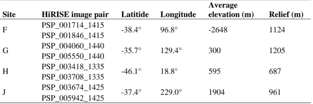
12 The precision of elevation values in the DEMs used here can be estimated based on 257

viewing geometry and pixel scale. For the DEM of site PC, the attendant image pair 258

PSP_004060_1440 (0.255 m/pixel) and PSP_005550_1440 (0.266 m/pixel) have a 12.6º 259

stereoscopic convergence angle. Assuming 1/5 pixel matching error and using a pixel scale of 260

0.266 m/pixel from the more oblique image, the vertical precision is estimated to be ~ 0.24 m 261

(cf. Kirk et al. 2008). DEMs for sites GC, KC and TS have a similar magnitude of vertical 262

precision. The pixel matching error is influenced by signal-to-noise ratio, scene contrast and 263

differences in illumination between images. Pattern noise can also be introduced by the 264

automatic terrain extraction algorithm, especially in areas of low correlation. Manual editing 265

is necessary to correct spurious topography in areas of poor correlation (e.g., smooth, low 266

contrast slopes and along shadows). 267

Finally, a synthetic crater was constructed to test whether the results from the Mars 268

study sites in general reflected the process, or instead were a result of the geometry imposed 269

by the impact crater setting (all the Mars study areas were on the inner walls of bowl shaped 270

depressions, but none of the ones on Earth were). A 10 km diameter synthetic crater was 271

created by applying a smooth parabolic radial profile, which was derived by fitting curves 272

through ungullied radial profiles of the craters in sites PC and GC. Metre-scale “pink” (also 273

called “1/f”) noise was added to simulate a natural rough surface (Jack 2000). 274

Derivation of drainage area and local slope

Representative slope sections were chosen in each DEM (Figs. 3 and 4). For Earth, these 276

were chosen to represent end member and intermediate process domains, including dry mass 277

wasting, debris flow and alluvial processes. On Mars, some areas were chosen that covered 278

the complete slope on which gullies are found, whilst others covered a single gully system, or 279

ungullied slope for comparison. Slope sections always included the drainage divide at the top 280

and extended downslope as far as the visible signs of the distal extent of the gully (or slope) 281

13 deposits. Where possible lines delineating drainage basins were followed to define the lateral 282

extent of slope sections, but on poorly incised hillslopes this was not always possible and the 283

lateral extent was defined as a straight line. For site KC, on Mars, we chose different 284

configurations of slope sections to test the sensitivity of our analyses to the exact method 285

used to delineate the slope-sections. Careful delineation of slope sections is necessary for two 286

reasons. Firstly, because the larger the sample area, the more processes are included within it, 287

and the more difficult the results will be to interpret. Secondly, if parts of the slope that are 288

integral to the process to be identified are omitted, then the process signal will not be 289

complete. 290

The slope and the flow directions of each pixel in each DEM were determined using 291

a “Dinf” algorithm. This algorithm gives flow directions in any direction, rather than only 292

towards one of the eight neighbouring pixels (Tarboton et al. 1991). This has been shown to 293

produce better results from slope-area analysis because it gives a more accurate 294

approximation of the real path of flow through the landscape (Borga et al. 2004). For each 295

pixel, the accumulation of flow was calculated from the flow directions by summing the 296

number of pixels located upstream, and multiplying by the pixel area. These analyses were 297

performed using the TauDEM extension for ArcGIS, based on the algorithms developed by 298

Tarboton (1997). For each DEM the “wetness index” was also calculated. This is the natural 299

logarithm of the ratio of contributing area to slope. It provides information on the potential 300

connectivity of the landscape drainage and the potential ability of the surrounding landscape 301

to route drainage (Woods & Sivapalan 1997). However, in the case of Earth and particularly 302

in the case of Mars this index should not be interpreted literally as implying that the terrain is 303

“wet”. In our study it is used as a visual aid to interpret the spatial variability of the slope-304

area plot. For example, highly permeable talus slopes on Earth are essentially dry, but they 305

may have moderate to high wetness index. However, we would expect a talus slope on Earth 306

14 to show a characteristic spatial pattern of wetness index, indicative of dry mass wasting 307

processes. All the DEMs underwent the same processing steps. 308

We extracted the drainage area and slope for every pixel within the chosen slope 309

sections. To simplify the representation of these data we calculated the mean slope for 0.05 310

wide logarithmic bins of drainage area, and then constructed the slope-area and CAD plots. 311

Binning data in this way make the trends in slope-area and CAD plots clearer and is a 312

commonly used display technique (e.g., Snyder et al. 2000). 313

In addition, for one site on Mars (site KC), we visually identified the initiation sites 314

of the gullies on orthorectified HiRISE images. The initiation points for the gullies were 315

defined as the furthest upstream extent defined by a distinct cut, or scarp (Fig. 5a). For each 316

of these locations we extracted the slope and drainage area for the underlying pixel. This 317

analysis was not performed for site PC because edge contamination and noise made it 318

impractical. The analysis was also omitted for site GC because the gullies start at the top of 319

the slope, so would by definition occur at the lowest drainage areas. 320

Study areas

Earth

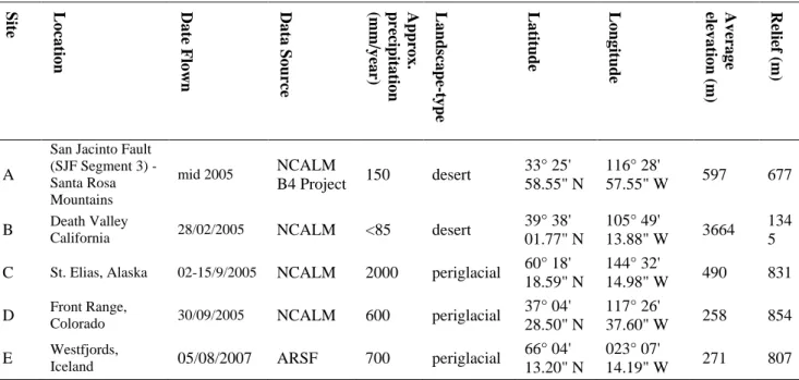
All the study sites on Earth are located in the northern hemisphere and most are within the 323

continental USA. Table 1 provides a summary of the sites and Fig. 3 shows the setting of the 324

areas studied. 325

Site SJ – San Jacinto, California 326

This site is located in California along a splay of the San Andreas fault, called the San Jacinto 327

fault. This area is a desert with little rainfall (~ 150 mm, annual average recorded by NOAA 328

weather station in nearby Borrego Springs), which has undergone rapid recent uplift caused 329

15 by the fault system. The landscape has a well developed ephemeral gully network with large 330

alluvial fans. From the study of the 1 m LiDAR data and aerial images we infer the processes 331

forming these fans to be sheet-flow rather than debris flow, based on the lack of levées and 332

lobate terminal deposits. The vegetation is sparse, consisting of small scrub bushes. The 333

underlying geology of the study area is mainly granite, schist and gneiss with minor outcrops 334

of Quaternary older fan deposits (Moyle 1982). For our analyses we used three study areas 335

that contained small complete gully systems, including sources, channels and debris aprons, 336

but avoided large fan systems and debris aprons from neighbouring systems (Figs. 3a and 3b: 337

study areas SJ1, SJ2 and SJ3). Due to the small size of the fans in area SJ1 it is difficult to 338

entirely rule out debris flow as a potential process in forming these alluvial fans. 339

Site DV - Death Valley, California 340

This site is located a few kilometres NE of Ubehebe volcano, in Death Valley, California. 341

This is a desert area that has well developed ephemeral gully networks with large alluvial 342

fans. There is little precipitation in this area although the nearby mountains receive as much 343

as 85 mm of rain per year (Crippen 1979) and rare large storms can do much geomorphic 344

work. Debris flows are found on the fans in the area (e.g., Blair 1999, 2000), but the primary 345

process active in the gullies is alluvial transport (Crippen 1979). We inspected the 1 m 346

LiDAR data for presence of levées and depositional lobes on the fans and found no evidence 347

of these. However, without direct field observations the fact that debris flows do not act on 348

these fans remain an assumption. The bedrock consists of Palaeozoic sedimentary rocks 349

(Workman et al. 2002). We chose two study areas (Fig. 3c: study areas DV1 and DV2) with 350

gully systems that were not affected by neighbouring alluvial fans or gully systems so only 351

receive local rainfall levels. 352

16 Site KA – St Elias Mountains, Alaska

353

This site is located east of the abandoned town of Katalla close to the recently deglaciated 354

mountain range of St Elias, near the coast of Alaska and on the border with Yukon, Canada. 355

The area has been unglaciated for approximately the last 10 000 years (Sirkin & Tuthill 1987) 356

and receives very high precipitation, which falls as snow on the upper slopes and rain on the 357

lower. Our study area overlies Tertiary volcanic materials. The slope scarp was generated by 358

the active Ragged Mountain Fault (Miller 1961). The area was neither snow covered nor tree 359

covered at the time of survey and the slopes are composed of steep bedrock cliffs that lead 360

directly into large talus aprons. Debris flow tracks are apparent across this talus slope, 361

especially in study areas KA3 and KA4, and might have occurred in study area KA3 as well 362

(Fig. 3d). Study area KA1 has no evidence of debris flow processes (Fig. 3d). 363

Site FR – Front Range, Colorado 364

This site is located in the mountainous eastern side of the continental divide. The area was 365

deglaciated around 14 000 to 12 000 years before present (Godt & Coe 2007) and the 366

landscape is dominated by glacially carved valleys. This area has experienced recent debris 367

flows (Coe et al. 2002; Godt & Coe 2007) and has no permanent snowpack. Our study 368

slopes, located above the tree line, are dominated by Precambrian biotitic gneiss and quartz 369

monzonite, scattered Tertiary intrusions, and by various surface deposits, all of which host 370

debris flows (Godt & Coe 2007). The head and sidewalls of the cirques have large rockfall 371

talus deposits and which have also experienced recent debris flows. These slopes have little 372

or no vegetation. Three of our study areas (Figs. 3e and 3f: study areas FR2 to FR4) include 373

debris flows located on talus. By way of contrast, we also examined a partially vegetated 374

slope (study area FR1) that is unchanneled and which we infer to be dominated by creep 375

processes (Fig. 3e). 376

17 Site WF – Westfjords, Iceland

377

The site is located in NW Iceland and is dominated by fjords and glacially carved valleys. 378

The last glacial retreat occurred approximately 10 000 years before present (Norðdalh 1990). 379

The valley walls have many active debris flows (Conway et al. 2010b) and on the slopes 380

above Ísafjörður (Fig. 3g: study area WF1) they occur in most years (Decaulne et al. 2005). 381

The site has a maritime climate, so has high levels of both snow and rainfall, but does not 382

have permanent ice or snow patches. The site is underlain by Miocene basalts, although the 383

debris flows occur most often in glacial till. From this site we chose a study area above the 384

town of Ísafjörður that has very active debris flows (Fig. 3g: study area WF1), two study 385

areas with less active debris flows and more alluvial processes (Figs. 3g and 3h: study areas 386

WF2 and WF3), and one study area dominated by rockfall and rock slide processes, although 387

there are some debris flow tracks visible in the field (Fig. 3h: study area WF4). All these 388

study areas have patchy vegetation, but no trees. 389

Mars

All the gullies that we studied on Mars were located on the inner walls of craters in the 391

southern hemisphere (Table 2). Slopes both with and without gullies were analysed for 392

comparison. Sites PC, GC and KC were analysed by Lanza et al. (2010), because all the sites 393

showed visual evidence of debris flows. 394

Site PC – Penticton Crater in Eastern Hellas 395

This site contains the very recent, light-toned deposits observed by Malin et al. (2006) and 396

interpreted by them to be a recent “gully forming” event. These flows were later suggested by 397

Pelletier et al. (2008) to be produced by dry granular flow, or possibly also debris flow. This 398

slope does not have any well defined channels. We used two study areas within the ~ 7.5 km 399

diameter crater for our slope-area analyses, shown in Figs. 4a and 4b. Study area PC1 is 400

18 located over the equator-facing light-toned deposits (Fig. 4a) and study area PC2 on the west-401

facing crater wall which contains small gullies (Fig. 4b). These gullies appear to be incised 402

into “mantle deposits” (Mustard et al. 2001). The mantle is hypothesised to be the remnants 403

of a previously extensive volatile rich deposit (e.g., Mangold 2005). This crater is very 404

asymmetric, with the east and north rims being subdued in terms of elevation (the rim is 405

nearly absent on the east side) whilst the southern rim is abrupt and steep. 406

Site GC – Gasa Crater in Terra Cimmeria 407

This ~ 7 km wide crater, shown in Figs. 4c and 4d, has well developed alcoves or 408

indentations into the rim of the crater. Gully channels are most obvious on the west-facing to 409

pole-facing slopes (Figs. 4c and 4d) and the equator-facing slope lacks these well defined 410

alcoves and channels (Fig. 4e). We chose sections on the pole- (study areas GC1 and GC2), 411

west- (study area GC3) and equator-facing (study area GC4) slopes. This crater is located 412

within a larger crater, which also has gullies on its west- to pole-facing slopes. There is no 413

evidence of mantle deposits being present anywhere within this crater. 414

Site KC – crater inside Kaiser Crater in Noachis Terra 415

The study crater, ~ 12 km across is located within the larger Kaiser crater, which not only has 416

gullies down its own rim, but also gullies on the dunes within it (Bourke 2005). Gullies in 417

this crater have alcoves at various positions on the slope, which converge to form well 418

defined tributary networks. Lateral levées bound some of the channels (Figs. 5b and 5c). This 419

slope has the subdued appearance often attributed to the presence of volatile rich mantle 420

deposits (Mustard et al. 2001). We chose study areas that encompass the drainage area of two 421

gullies (study area KC2), a single gully (study area KC1) and also the slope section as a 422

whole (study area KC3), all of which are shown in Fig. 4f. We chose study area KC4, an area 423

of the slope not affected by gullies, for comparison (Fig. 4f). 424

19 Site TS – crater in Terra Sirenum

425

This ~ 7 km diameter crater is located to the south of Pickering Crater in Terra Sirenum and 426

contains pole-facing gullies. We analysed an equator-facing slope (Fig. 4g: study area TS1) 427

which has no evidence of channels but contains an apparently well developed talus apron. 428

There is no evidence of mantle deposits being present on this slope. 429

Results

Earth

Initially we chose two study areas with talus and with active creep. The slope-area analysis 432

results for these are shown in Fig. 6a. The study areas with well developed talus (WF4 and 433

KA1) show the following pattern on log-log plots: (1) At small drainage area the curves are 434

initially flat. (2) There is then a linear decrease in slope with increasing drainage area. (3) The 435

curve then becomes horizontal again at higher drainage area with a lower slope value. Talus 436

slopes that have a mixture of processes (e.g., KA2) show a curve that drops off linearly in 437

log-log plots then flattens at higher drainage areas. 438

The CAD plot (Fig. 7a) provides additional information: the talus dominated study 439

areas have a very smooth convex shape. The gradient of the curve is low until the drainage 440

area is between approximately 0.001 km2 after which the curve drops sharply and continues 441

to steepen with increasing drainage area. 442

The soil creep diffusive process study area (FR1 in Fig. 6a) shows a distinctive 443

signature in slope-area plots: (1) The curve is initially horizontal to gently downwards 444

sloping. (2) Between drainage areas of 0.0001 to 0.001 km2 the slope increases linearly with 445

increasing drainage area. (3) There is then a marked slope turnover at which the curve 446

switches to decreasing slope with increasing drainage area. The soil creep diffusive process 447

study area resembles the talus slopes in CAD plots (FR1, Fig. 7a). 448

20 Figs. 6b and 7b show the debris flow study areas that are influenced by talus 449

processes and Figs. 6c and 7c show those that are more influenced by alluvial processes. 450

Generally in slope-area plots debris flow produces a curve that drops off linearly in log-log 451

plots, flattening off before finally dropping away steeply. The difference between the talus 452

study areas (e.g. KA2, Fig. 6a) and the debris flow study areas influenced by talus (Fig. 6b) is 453

subtle in some cases. In a similar way the difference between the debris flow areas influenced 454

by talus processes (Fig. 6b) and those influenced by alluvial processes (Fig. 6c) is also subtle. 455

Without field information it would be difficult to differentiate talus dominated and debris 456

flow dominated slopes reliably in slope-area plots (e.g., compare Figs. 6a, KA2 and 6b). 457

However, in CAD plots it is possible to differentiate between the two process types. The 458

debris flow dominated study areas (Figs. 7b and 7c) show the following pattern: (1) The 459

curve drops away from the horizontal slowly (but faster than the talus slopes) at small 460

drainage areas. (2) The curve then either dips down linearly, or follows a flattened convex 461

path, and (3) at high drainage areas the curve drops away sharply with increasing drainage 462

area. 463

Study areas modified by ephemeral water flow have distinct signatures in slope-area 464

plots (Fig. 6d) and in CAD plots (Fig. 7d). In slope-area plots they show a shallow linearly 465

decreasing trend at small drainage areas, which gets steeper at higher drainage areas, and 466

drops into the alluvial domain. The CAD plot drops away from the horizontal slowly and then 467

dips down linearly (or even with a concave profile) until the tail of the curve drops sharply 468

off at the highest drainage areas. 469

Synthetic Crater

The slope-area and CAD plots for the synthetic crater are easily differentiated from the 471

process study areas that we have examined on Earth. In slope-area plots the synthetic crater 472

produces a hump-backed curve (Fig. 8d): at small drainage areas the curve rises steeply, then 473

21 levels off and drops at high drainage areas. In appearance the curve is, as expected, nearest to 474

study area FR1, the area dominated by diffusive creep (Fig. 6a). In CAD plots (Fig. 9d) the 475

line follows a smooth convex arc, similar to that shown by talus on Earth, except without a 476

break in gradient. 477

Mars

The slope-area plots for sites PC and GC (Penticton Crater and Gasa Crater inner slopes) 479

closely resemble each one another (Fig. 8a and b). The resulting curve can be divided into 480

three zones: (1) A short initial increase in slope with increasing drainage area, followed by a 481

slope turnover at very small drainage areas. (2) A linear or slightly concave decreasing slope 482

trend with increasing drainage area that continues for most of the plot. (3) Finally, at the 483

largest drainage areas, there is a steep decrease in slope with increasing drainage area. For 484

study area PC1 there is a distinct and linear decline in slope with drainage area, whereas for 485

study areas PC2, GC1, GC2 and GC3 this section is slightly concave. The drop-off at the 486

highest drainage areas occurs at lower absolute drainage area values than for site GC. In the 487

CAD plot, study areas PC1 and GC4 have a smooth convex form, whereas study areas PC2, 488

GC1 and GC2 all have a nearly linear, flattened section at intermediate drainage areas (Figs. 489

9a and 9b). Study area GC3 lies close to PC1, GC1 and GC2 but without any sign of 490

flattening. 491

The slope-area plots for gullies in study areas KC1, KC2 and KC3 (Fig. 8c) can be 492

split into three sections as follows: (1) at small drainage areas the curve is sub-horizontal with 493

a subtle upward trend. This trend is more apparent for the data from individual gullies than 494

the data obtained from the whole slope section and is somewhat variable between gully 495

systems. (2) At intermediate drainage areas there is a transitional zone, occurring at different 496

drainage areas for each gully system, in which slope drops off markedly with drainage area. 497

22 (3) At higher drainage areas there is a gently declining relationship between slope and 498

drainage area, which is the same for all the gully systems. 499

The ungullied study area (KC4) is also shown in Fig. 8c. This study area has a 500

hump-back shape, resembling that seen for the synthetic crater. The hump occurs across the 501

same slope values as the transition zone (2) for the gullied slopes. In CAD plots (Fig. 9c) 502

study areas KC2 and KC3 have a flattened section at intermediate drainage areas, followed 503

by a steepening decrease at higher drainage areas. The study area without gullies (KC4) has a 504

curve that is convex and initially declines slowly, before dropping off steeply. Study area 505

KC1 has a less flattened profile than study areas KC2, or KC3 and it seems to be a mixture 506

between slope types typified by gullied study areas KC2 or KC3 and ungullied study area 507

KC4. 508

In slope-area plots, study area TS1, an ungullied slope, shows a slope-area turnover 509

at small drainage areas, followed by a decreasing and slightly concave trend in slope with 510

drainage area (Fig. 8d). There is a slight upturn at the highest drainage areas, but this is likely 511

to be an artefact caused by few data-points being used to calculate the mean slope in these 512

bins. In CAD plots (Fig. 9d) study area TS1 has a very smooth convex curve. 513

The slope and drainage area of the gully head initiation points were recorded for site 514

KC. These data are displayed on Fig. 8c. Interestingly, the locations of the gully heads cluster 515

around the range of drainage areas of the transitional section in the slope-area plot, but are 516

located at higher slope values. 517

Wetness Index on Earth and Mars

The spatial distribution of the slope-area data is most easily visualised using a wetness index 519

map. Maps of wetness index are presented for Earth (Fig. 10) and for Mars (Fig. 11). The 520

alluvial study areas in Earth sites SJ and DV show very low overall wetness indices – only 521

the channels have significant wetness index (Figs. 10a, 10b, and 10c). Debris flow study 522

23 areas are slightly more complex (Figs. 10d, 10e, 9f, 10g, and 10h): the slopes generally have 523

moderate wetness index, but there are localised paths along which the wetness index is 524

higher. Site WF (Figs. 10g and 10h) is the best example of this pattern, but it is also the area 525

with the highest influence of overland flow. For site KA (Fig. 10d) this signature is poorly 526

developed, but this site has been influenced by talus processes. The creep dominated study 527

area, FR1, has moderate wetness index throughout (Fig. 10e). The talus study areas KA1, 528

KA2 (Fig. 10d) and WF4 (Fig. 10h) show lobe-like areas of low wetness index with widening 529

streaks of higher wetness index in between. 530

On Mars, study area PC1 (Fig. 11a) and the synthetic crater (Fig. 11h) have similar 531

wetness index maps: the slope generally increases in wetness index going downhill and there 532

are quasi-linear streaks of higher wetness index that increase in value going downslope. 533

Study area PC2 (Fig. 11b) has overall low wetness index, apart from concentrated lines of 534

high wetness index within the gully alcoves, that spread and become more diffuse in the 535

debris aprons. A similar overall pattern is shown for study areas GC1, GC2 and GC3 (Figs. 536

11c and 11d), but the ridges around the alcoves have very low wetness index. Study area GC2 537

in particular (Fig. 11c) shows very concentrated slightly sinuous high wetness index lines on 538

its debris apron. However this part of the DEM contains significant noise, making it hard to 539

judge whether this is simply an artefact. Study areas GC4 (Fig. 11e) and TS1 (Fig. 11g) have 540

similar wetness index maps: there is low wetness index at the crest of the slope and where 541

bedrock is exposed and the wetness index generally increases downslope, but this trend is 542

superposed with diffuse linear streaks of higher relative wetness index. Site KC (Fig. 11f) has 543

generally moderate wetness index, with the alcoves and channels of the gullies showing 544

focussed high wetness index flanked by much lower wetness index and the debris aprons 545

having generally high wetness index with diffuse downslope streaking. 546

24

Discussion

547

Comparison of Earth data to previously published slope-area

process domains

There are two interlinked methods of determining slope processes from slope-area plots: 550

(1) The data points fall within domains in the plots which have been found both theoretically 551

and empirically to relate to particular processes, and 552

(2) The data points exhibit trends and gradients that provide information on active processes. 553

We compared our data from Earth to the slope-area process domains of Montgomery 554

& Foufoula-Georgiou (1993) and the additional domain added by Brardinoni & Hassan 555

(2006), shown as solid lines in Fig. 6. The data from our creep, talus and debris flow analyses 556

fall into the debris flow domain of Montgomery & Foufoula-Georgiou (1993). However, 557

some of our debris flow data drop into the alluvial domain at the highest drainage areas. 558

Because they are small systems with limited drainage areas, however, only a few points fall 559

within the alluvial domain. Some of our data approach the additional domain added by 560

Brardinoni & Hassan (2006), but do not extend towards sufficiently high drainage areas (or 561

low drainage areas) to enter it (Fig. 6b and 6c). Our data from the alluvial systems (Fig. 6d) 562

fall into both the debris flow and alluvial domains. They start to trend downwards in slope-563

area plots at lower drainage areas than our debris flow systems. 564

Tucker & Bras (1998) simulated the effects of different dominant processes on 565

slope-area plots and we now compare their model results to the patterns in slope-area plots 566

shown by our data. Our talus systems (Fig. 6a) closely fit their model of a landscape 567

dominated by landsliding (which includes the process of debris flow). In slope-area plots our 568

talus data have an initial flat section at small drainage areas, which represents the slope 569

threshold for the rock wall failure and so differs between localities. At higher drainage areas 570

25 the curves are again flat, representing the failure threshold of loose talus, which is consistent 571

for all areas at approximately 0.7 gradient, equivalent to a slope of approximately 35°. This is 572

an approximate mean slope angle for talus slopes on Earth (Chandler 1973; Selby 1993) and 573

is shown by a dotted horizontal line in Figs. 6 and 8. Between these two horizontal sections 574

there is a transition where the dominance shifts from rock wall failure to unconsolidated talus 575

failure. 576

Within the framework of Tucker & Bras (1998) the pattern shown by the debris flow 577

slopes on Earth (Figs. 6b and 6c) is most consistent with the transition from unsaturated 578

landsliding (dry mass wasting of both talus and rock wall) to pore pressure triggered 579

landsliding (which we interpret to also include debris flow), in a landscape dominated by 580

landsliding. The presence of processes with a slope failure threshold cause data in slope-area 581

plots to fall along horizontal lines. Hence, as the process dominance changes from rock wall 582

failure (highest threshold) to unsaturated landsliding (intermediate threshold) to saturated 583

landsliding (lowest threshold) the curve declines and levels off at the slope value of the 584

saturated landslide threshold in that particular area. As each physical locality has its own 585

saturation threshold this horizontal section occurs at different slope values for different 586

localities but is always located below the dry stability line at 0.7. 587

In slope-area plots, our data from alluvial systems on Earth (Fig. 6d) show a simple 588

decline of slope with drainage area, possibly steepening at higher drainage areas. The data are 589

scattered at drainage areas > 0.001 km2, due to the limitations of the small sizes of the gully 590

systems available. This means a relatively small number of pixels were used to generate each 591

point, leading to random scatter. However, even taking into account the scatter, the data are 592

below the slope threshold for dry slope failure at 0.7 gradient, which suggests a gradual 593

transition from pore pressure dominated landsliding to fluvial processes. 594

26 The main feature of our creep dominated hillslope data (FR1, Fig. 6a), is a turnover 595

from increasing slope with drainage area to decreasing slope with drainage area. One of the 596

alluvial systems in site SJ (study area SJ3) shows a weak slope turnover at the lowest 597

drainage areas but none of the other plots show this feature. The slope-area turnover is shown 598

in Fig. 2 and is generally expected to occur in slope-area plots (e.g., Tucker & Bras 1998). It 599

usually occurs in, or close to, the “hillslope” domain of Montgomery & Foufoula-Georgiou 600

(1993). The turnover represents a transition from convex slopes dominated by diffusive 601

processes (which include soil creep often modified by plant roots and other biota) to concave 602

slopes dominated by advective, or alluvial processes. Within the diffusive processes domain 603

in slope-area plots, slope increases with drainage area. The most likely reason that most of 604

our data do not show this turnover is that the slopes we studied lack stable vegetation 605

(Dietrich & Perron 2006; Marchi et al. 2008). Another potential contributing factor is that the 606

bedrock and colluvium in our study areas are not naturally cohesive, for example, clay-rich 607

rocks can exhibit convex creep-dominated slopes in unvegetated badlands on Earth. 608

The pattern of data in slope-area plots shown by our alluvial systems and some of 609

our debris flow systems (slow decline at small drainage areas followed by a steep decline at 610

higher drainage areas) has been shown from numerous remote sensing and field studies to 611

mark the transition from the colluvial (including debris flow) regime, to that of a fully fluvial 612

regime (e.g., Lague & Davy 2003; Stock & Dietrich 2003; Stock & Dietrich 2006). Some 613

have described the transition as a separate linear portion of the plot between the colluvial and 614

the fluvial (Lague & Davy 2003) and some as a gradual curved transition (Stock & Dietrich 615

2003). However, both are consistent with Tucker & Bras’ (1998) transition from pore 616

pressure triggered landsliding into a fully fluvial system. Our plots do not show a well 617

developed alluvial regime, but this is due to the use of high resolution data of very small 618

areas rather than large, well developed fluvial catchments. 619

27 In summary, our terrestrial data are consistent with published slope-area process 620

domains, and provide reassurance that the method is applicable and that the Mars data can be 621

used to infer process in a similar way. The caveat to this is that the environmental differences 622

between Earth and Mars, as detailed in the introduction, must be considered when comparing 623

terrestrial process domains to data from Mars. Furthermore, improved process discrimination 624

can be made by considering CAD profiles in addition to slope-area analysis. 625

Comparison of Earth data to published CAD process domains

Comparison of all our CAD plots for Earth (Fig. 7) to the published process domains for 627

CAD (Fig. 2) reveals that our data do not generally follow the cited trends. This is possibly 628

because we are studying small areas, rather than large catchments. However, the shape of the 629

curve outlined by our data in CAD plots does allow process discrimination and does follow 630

some of the framework outlined by McNamara et al. (2006). Specifically region 1 on Fig. 2 631

has three sub-regions whose shapes can be recognised in our datasets. The talus data (Fig. 7a) 632

and synthetic crater (Fig. 9d) are both convex in their CAD plots, resembling most closely 633

region 1a of McNamara et al. (2006). They describe this region as representing “hillslopes 634

that diverge and do not gather drainage.” Our alluvial data and some of our debris flow data 635

show a flattening of the CAD plot curve in the middle region, giving a steep linear section, 636

corresponding to either region 1b or region 2 (Fig. 2b) which McNamara et al. (2006) 637

describe as slopes that are convergent (1b), or channel forming (2). Two debris flows (WF2 638

and WF3 in Fig. 7c) show a concave section, which would correspond to region 1c of 639

McNamara et al. (2006) and which they attribute to pore pressure triggered landsliding or 640

debris flow. 641

The similarity of talus and debris flow in slope-area plots can be attributed to their 642

similarly linear long profiles. However, the two processes produce different patterns in CAD 643

28 plots because talus slopes tend to disperse drainage but debris flow slopes tend to have 644

convergent drainage. This can also be seen in the wetness index plots (Fig. 10). 645

This difference of behaviour in CAD and wetness index plots, in addition to the 646

information from the slope-area plots, shows that we can detect slopes dominated by alluvial, 647

debris flow and dry mass wasting on the basis of these parameters, even for small catchments 648

such as individual gullies or debris flow tracks. However, it should be noted here that these 649

analyses have been performed on relatively few sample sites on Earth and some of the 650

differences are subtle. Future work has to include extending this analysis to a greater number 651

of test sites on Earth to verify that this kind of process discrimination is robust. Using these 652

initial results we continue and apply these methods of process discrimination to Mars. 653

Process domains for gullies on Mars

In slope-area plots all the Mars slope sections, except study area TS1, fall below the slope 655

threshold for dry mass wasting (dotted line in the plots in Fig. 8). This means that talus-like 656

dry mass wasting is not a dominant process in these areas. However, study area TS1, visually 657

similar to talus on Earth, is not only above the slope threshold for dry mass wasting, but also 658

bears a signature similar to talus on Earth in the combination of its slope-area plot, CAD plot 659

and wetness index map 660

Within the process domains of Montgomery & Foufoula-Georgiou (1993) the 661

majority of the Mars data lie within the debris flow domain, with some data located in the 662

debris flow deposition domain added by Brardinoni & Hassan (2006) and a few in the 663

alluvial domain. The difference in gravity between Earth and Mars requires an upwards slope 664

adjustment to the alluvial channels domain boundary (see Fig. 2a) in slope-area plots 665

(Appendix 1), but does not change the gradient of the line. This is marked by the dash-dot 666

line on the plots in Fig. 8. This shift places more data in the unchanneled domain, but does 667

not place any additional data into the alluvial or debris flow domains. This in itself 668

29 distribution does not provide very detailed information on the formation mechanisms for 669

gullies. However, by combining slope-area trends, CAD plots and wetness index maps we 670

can make more detailed assessments. We examine each of the study areas on Mars in turn 671

and then discuss the overall implications for the gully formation processes. 672

Synthetic Crater 673

The pattern in slope-area plots of the interior of impact craters is, in part, a result of 674

the inherent shape of the crater slope which in turn is due to the impact process and the 675

modification that occurs immediately afterwards. The slope of a fresh impact crater is 676

concave and exponentially shaped in profile (Garvin et al. 1999). Thus in slope-area plots it 677

resembles a well developed alluvial system on Earth (e.g., Hack 1957). This reinforces the 678

uncertainty in inferring a unique process from slope form. In CAD plots, however, the 679

synthetic crater data show a similar pattern to that of talus slopes on Earth, indicating that at 680

short length-scales this type of slope cannot channelise flow on its own. This interpretation is 681

supported by the wetness index plot (Fig. 11), which shows a slowly coalescing flow, rather 682

than discrete areas of fluid concentration. 683

Site PC – Penticton Crater in Eastern Hellas 684

In slope-area plots the slope turnover is well expressed for both study areas in site 685

PC (Fig. 8a). This suggests a strong diffusive or creep influence on both slopes. Study areas 686

PC1 and PC2 both resemble either poorly developed talus or debris flow in slope-area plots. 687

In the CAD plot (Fig. 9a); however, study area PC2 has the distinctive profile associated with 688

debris flow, whereas study area PC1 more closely resembles talus. Talus processes can only 689

be active in study area PC1 at small drainage areas, where it lies on the dry mass wasting 690

threshold in slope-area plots. Hence the shape of the CAD curve must be explained by 691

another process, which has a slope threshold but does not concentrate drainage. This 692

30 unknown process must be pore pressure triggered as it is below the slope for dry mass 693

wasting. In addition, the wetness index plot reveals that study areas PC1 and PC2 are very 694

different: study area PC1 has a similar wetness index map to the synthetic crater (Fig. 11h), 695

whereas study area PC2 resembles debris flow areas on Earth (e.g., Fig. 10f) with strongly 696

concentrated high wetness index within alcoves and channels, becoming more diffuse down 697

slope on the debris aprons. 698

The combined evidence suggests that the west-facing slope, which contains small 699

gullies, has been modified by debris flow, whereas the equator-facing slope is more similar to 700

dry mass wasting deposits. This agrees with the interpretation of Pelletier et al. (2008), who, 701

using numerical modelling, concluded that the new bright toned deposits on this slope were 702

more similar in form to deposits of dry granular flows than debris flows. 703

Site GC – Gasa Crater in Terra Cimmeria 704

In the slope-area plot for site GC (Fig. 8b), the slope-turnover occurs at very small 705

drainage areas (one or two pixels) and is thus partly abbreviated. This suggests that creep has 706

not strongly influenced this site. This interpretation is supported by the observation that the 707

gully heads originate at the very top of the slope. Study areas GC1, GC2 and GC3 resemble 708

either poorly developed talus on Earth (study area KA2, Fig. 6a) or debris flows on Earth 709

(Figs. 6b and 6c) in slope-area plots. However, in CAD plots (Fig. 9b) they have a flattened 710

mid-section, resembling debris flow systems on Earth. Their wetness index plots (Figs. 11c 711

and 11d) have strong similarities with debris flow systems on Earth (e.g., Fig. 10g): showing 712

flow concentration in the alcove and channel with more diffuse flow on the debris apron. 713

Study area GC2 (Fig. 11c) shows a similar pattern of wetness index to the alluvial systems on 714

Earth, with focussed flow throughout. 715

In slope-area plots (Fig. 8b) study area GC4 has a flatter profile than study areas 716

GC1, GC2 and GC3. The drop in slope at high drainage areas in GC4 is probably an artefact 717

31 of the low number of pixels included in the slope calculations in the last 5 to 10 points. In the 718

CAD plot (Fig. 9b), study area GC4 has a similar shape to talus systems on Earth (Fig. 7a). 719

The talus interpretation for GC4 is supported by additional evidence: (1) there is no evidence 720

for channels (Fig. 4e), (2) the wetness index plot (Fig. 11e) is similar to talus slopes on Earth 721

and (3) part of the slope-area curve lies on the threshold for dry mass wasting (Fig. 8b). The 722

dip of the slope-area curve away from the threshold for dry mass wasting suggests that 723

another process with a lower slope threshold is acting, either without having an effect on the 724

CAD plot, or with the same CAD plot as talus. We hypothesise that this may be the same 725

unknown process as noted in study area PC1. 726

The combined evidence suggests that the pole and east facing slopes of the crater 727

have been affected by debris flow processes and the equator-facing slope by mass wasting 728

and an unknown process. 729

Site KC – crater inside Kaiser Crater in Noachis Terra 730

Our ungullied study area (KC4) shows patterns in slope-area (Fig. 8c) and CAD plots (Fig. 731

9c) very similar to the synthetic crater and creep slopes on Earth. The difference between this 732

study area and the gullied study areas (KC1 to KC3) is presumably a result of the process of 733

gully formation. Study areas KC1 to KC3 do not have slope-area plots (Fig. 8c) that fit easily 734

within the framework established so far. However, if we refer to the modelling work of 735

Tucker & Bras (1998) then the patterns in slope-area plots can be explained. At small 736

drainage areas our curves for study areas with gullies have a horizontal or slightly positive 737

trend compared to our ungullied study area, which has a definite positive trend. This suggests 738

the weak influence of diffusive processes (which generate a positive relationship in slope-739

area plots) combined with slope threshold processes (which tend to produce horizontal 740

trends). As all the data are below the dry mass wasting threshold, this threshold process is 741

likely to be a pore pressure triggered process, such as debris flow. At intermediate drainage 742

32 areas there is a transitional region which occurs at a similar drainage area to the slope-743

turnover in the ungullied section. At high drainage areas the gullied study areas show a 744

slightly decreasing sub-horizontal trend, as opposed to the ungullied study area which has a 745

well defined decrease in slope with drainage area. This also can be attributed to a pore 746

pressure triggered threshold process but at a lower slope threshold than the previous process. 747

In CAD plots (Fig. 9c) study areas KC1 to KC3 are consistent with debris flow processes. 748

The wetness index plots for these study areas (Fig. 11f) are similar to terrestrial debris flow 749

study areas which have been influenced by alluvial processes (e.g., site WF, Figs. 10g and 750

10h). This suggests that the first pore pressure threshold in slope-area plots is due to debris 751

flow and the second lower one due to an unknown process, which again could be the same 752

process affecting sites PC and GC. 753

In slope-area plots, the gully heads on this slope (Fig. 8c) coincide with the drainage 754

area of the slope turnover in study area KC4 and the transitional study areas of KC1 to KC3. 755

This coincident relationship matches the observations made by many authors who have 756

studied gullies on Earth (e.g., Hancock & Evans 2006). Our channel heads lie mainly in the 757

domain attributed to “pore pressure landsliding channel initiation” processes, but some also 758

lie in the “unchanneled” domain (McNamara et al. 2006). Notably the gully heads occur 759

below the dry mass wasting threshold, again suggesting that these martian gullies are initiated 760

by a pore pressure threshold process. The gully heads occur on slope gradients of 0.55 similar 761

to those described by Lanza et al. (2010), but at drainage areas an order of magnitude lower. 762

This is possibly due to the different approach used by Lanza et al. (2010) to measure the 763

contributing area, and possible differences in their interpretation of the location of channel 764

initiation. The co-occurrence of the gully heads with the slope-turnover in slope-area plots 765

suggests that the gullies are a result of whole-slope drainage, as previously found by Lanza et 766

al. (2010), either at the surface or shallow subsurface. Our work provides additional evidence 767