The MIT Faculty has made this article openly available.
Please share
how this access benefits you. Your story matters.
Citation
Chen, Zhe et al. “Discrete- and Continuous-Time Probabilistic
Models and Algorithms for Inferring Neuronal UP and DOWN
States.” Neural Computation 21.7 (2009): 1797–1862. Web.
As Published
http://dx.doi.org/10.1162/neco.2009.06-08-799
Publisher
MIT Press
Version
Author's final manuscript
Citable link
http://hdl.handle.net/1721.1/70846
Terms of Use
Creative Commons Attribution-Noncommercial-Share Alike 3.0
Discrete- and Continuous-Time Probabilistic Models and
Algorithms for Inferring Neuronal UP and DOWN States
Zhe Chen,
Neuroscience Statistics Research Laboratory, Department of Anesthesia and Critical Care, Massachusetts General Hospital, Harvard Medical School, Boston, MA 02114, U.S.A., and Department of Brain and Cognitive Sciences, Massachusetts Institute of Technology, Cambridge, MA 02139, U.S.A
Sujith Vijayan,
Program in Neuroscience, Harvard University, Cambridge, MA 02139, U.S.A., and Picower Institute for Learning and Memory, Massachusetts Institute of Technology, Cambridge, MA 02139, U.S.A
Riccardo Barbieri,
Neuroscience Statistics Research Laboratory, Department of Anesthesia and Critical Care, Massachusetts General Hospital, Harvard Medical School, Boston, MA 02114, U.S.A
Matthew A. Wilson, and
Picower Institute for Learning and Memory, RIKEN-MIT Neuroscience Research Center,
Department of Brain and Cognitive Sciences and Department of Biology, Massachusetts Institute of Technology, Cambridge, MA 02139, U.S.A
Emery N. Brown
Neuroscience Statistics Research Laboratory, Department of Anesthesia and Critical Care, Massachusetts General Hospital, Harvard Medical School, Boston, MA 02114, U.S.A., Harvard-MIT Division of Health Sciences and Technology, Cambridge, MA 02139, U.S.A., and Department of Brain and Cognitive Sciences, Massachusetts Institute of Technology, Cambridge, MA 02139, U.S.A
Zhe Chen: [email protected]; Sujith Vijayan: [email protected]; Riccardo Barbieri: [email protected]; Matthew A. Wilson: [email protected]; Emery N. Brown: [email protected]
Abstract
UP and DOWN states, the periodic fluctuations between increased and decreased spiking activity of a neuronal population, are a fundamental feature of cortical circuits. Understanding UP-DOWN state dynamics is important for understanding how these circuits represent and transmit information in the brain. To date, limited work has been done on characterizing the stochastic properties of UP-DOWN state dynamics. We present a set of Markov and semi-Markov discrete- and continuous-time probability models for estimating UP and DOWN states from multiunit neural spiking activity. We model multiunit neural spiking activity as a stochastic point process, modulated by the hidden (UP and DOWN) states and the ensemble spiking history. We estimate jointly the hidden states and the model parameters by maximum likelihood using an expectation-maximization (EM) algorithm and a Monte Carlo EM algorithm that uses reversible-jump Markov chain Monte Carlo sampling in the E-step. We apply our models and algorithms in the analysis of both simulated multiunit spiking activity and actual multiunit spiking activity recorded from primary somatosensory cortex in a behaving rat during slow-wave sleep. Our approach provides a statistical characterization of UP-DOWN state dynamics that can serve as a basis for verifying and refining mechanistic descriptions of this process.
NIH Public Access
Author Manuscript
Neural Comput. Author manuscript; available in PMC 2009 December 29. Published in final edited form as:
Neural Comput. 2009 July ; 21(7): 1797–1862. doi:10.1162/neco.2009.06-08-799.
NIH-PA Author Manuscript
NIH-PA Author Manuscript
1 Introduction
1.1 Neuronal State and Recurrent Networks
The state of the neural system reflects the phase of an active recurrent network, which organizes the internal states of individual neurons into synchronization through recurrent network synaptic activity with balanced excitation and inhibition.1 The neuronal state dynamics can be externally or internally driven. The externally driven dynamics results from either sensory-driven adaptation or encoding of sensory percept; the internally sensory-driven dynamics results from changes in internal factors, such as attention shift. Different levels of neuronal state also bring in the dynamics of state transition. Generally state transitions are network controlled and can be triggered by the activation of single cells, which are reflected by changes in their intracellular membrane conductance.
From a computational modeling point of view, two types of questions arise. First, how do neurons generate, maintain, and transit between different states? Second, given the neuronal (intracellular or extracellular) recordings, how can the neuronal states be estimated? The computational solutions to the first question emphasize the underlying neuronal physiology or neural mechanism, which we call mechanistic models, whereas the solutions to the second question emphasize the representation or interpretation of the data, which we call statistical models. In this article, we are taking the second approach to model a specific phenomenon regarding the neuronal state.
1.2 Neuronal UP and DOWN States
The notion of neuronal UP and DOWN states refers to the observation that neurons have two distinct subthreshold membrane potentials that are relevant for action potential (i.e., spike) generation. A neuron is said to be depolarized (or excited) if its intracelluar membrane potential is above the resting membrane potential threshold (around −70 to −80 mV) and is said to be hyperpolarized (or inhibited) if its membrane potential is below the threshold. When a sufficient level of excitation is reached, a spike is likely to occur. Essentially, membrane potential fluctuations define two states of the neocortex. The DOWN state defines a quiescent period during which little or no activity occurs, whereas the UP state corresponds to an active cortical state with depolarized membrane potentials and action potential firing driven by synaptic input. It was generally believed that the spontaneous UP and DOWN states are generated by a balance of excitatory and inhibitory neurons in recurrent networks (Haider, Duque, Hasentaub, & McCormick, 2006). In recent years, many neurophysiological studies have been reported regarding the neuronal UP and DOWN states, ranging from intracellular or extracellular recordings (e.g., Sanchez-Vives & McCormick, 2000; Haider, Duque, Hasentaub, Yu, & McCormick, 2007). The UP and DOWN states that are characterized by the cortical slow oscillation in intracellular membrane potentials are also reflected in extracellular recordings, such as local field potential (LFP) or electroencephalograph (EEG), single-unit activity or multiunit activity (MUA). In the literature, the UP and DOWN states have been characterized by examining extracellular LFP recordings (Sirota, Csicsvari, Buhl, & Buzsáki, 2003; Battaglia, Sutherland, & McNaughton, 2004; Wolansky, Clement, Peters, Palczak, & Dickson, 2006) in either the somatosensory cortex of anesthetized or awake animals (e.g., Haslinger, Ulbert, Moore, Brown, & Devor, 2006; Luczak, Barthó, Marguet, Buzsáki, & Harris, 2007) or the visual cortex of nonanesthetized animals during sleep (e.g., Ji & Wilson, 2007). Recently, attention has also turned to multiunit spike trains in an attempt to relate spike firing activities with EEG recordings (Ji & Wilson, 2007).
1The neuronal state sometimes can refer to a single cell level, during which neurons exhibit different lengths or durations of depolarizing shift (e.g., Fujisawa, Matsuki, & Ikegaya, 2005).
NIH-PA Author Manuscript
NIH-PA Author Manuscript
In order to examine the relationship between sleep and memory in rats or animals, simultaneous recordings are often conducted in the neocortex and hippocampus with the goal of studying the cortico-hippocampal circuit and the functional connectivity of these two regions while the animals perform different tasks. It has been reported (e.g., Volgushev, Chauvette, Mukovski, & Timofeev, 2006) that during the slow wave sleep (SWS), which is characterized by 0.5 to 2.0 Hz slow oscillations (Buzsáki, 2006), neorcortical neurons undergo near-synchronous transitions, every second or so, between UP and DOWN states. The process of the alternating switch between the two states appears to be a network phenomenon that originates in the neocortex (Ji & Wilson, 2007; Vijayan, 2007).
The work reported here was driven by the experimental data accumulated in our lab (Ji & Wilson, 2007; Vijayan, 2007). The growing interest in UP and DOWN states in the
neuroscience literature motivated us to develop probabilistic models for the UP and DOWN modulated MUA. Specifically, the UP-DOWN states are modeled as a latent two-state Markovian (or semi-Markovian) process (Battaglia et al., 2004), and the modeling goal is to establish the probability for state transition or the probability density of UP or DOWN state duration and the likelihood model that takes into account both a global hidden state variable and individual history dependence of firing. In comparison with the standard and deterministic threshold-based method, our proposed stochastic models provide a means for representing the uncertainty of state estimation given limited experimental recordings.
1.3 Markov and Semi-Markov Processes and Hidden Markov Models
A stochastic process is said to be Markovian if it satisfies the Markov property; the knowledge of the previous history of states is irrelevant for the current and future states. A Markov chain is a discrete-time Markov process with the Markov property. The Markov process and Markov chain are both “memoryless.” A Markov process or Markov chain contains either continuous-valued or finite discrete-continuous-valued states. A discrete-state Markov process contains a finite alphabet set (or finite state space), with each element representing a distinct discrete state. The change of the state is called the transition, and the probability of changing from one state to the other is called the transition probability. For the Markov chain, the current state has only finite-order dependence on the previous states. Typically the first-order Markov property is assumed; in this case, the probability of Sk+1 being in a particular state at time k + 1, given
knowledge of states up to time k, depends on the state Sk at time k, namely, Pr(Sk+1 ∣ S0, S1, …, Sk) = Pr(Sk+1 ∣ Sk). A semi-Markov process (the Markov renewal process) extends the
continuous-time Markov process to the condition that the interoccurrence times are not exponential.
When the state space is not directly observable, a Markov process is called hidden or latent. The so-called hidden Markov process is essentially a probabilistic function of the stochastic process (for a review, see Ephraim & Merhav, 2002). In the discrete-time context, the hidden Markov model (HMM) is a probabilistic model that characterizes the hidden Markov chain. The HMM is a generative model in that its full model {π, P, B} (where π denotes the initial state probability, P denotes the transition probability, and B denotes the emission probability) completely characterizes the underlying probabilistic structure of the Markov chain. Generally several conditions are assumed in the standard HMM: (1) the transition and emission probabilities are stationary or quasi-stationary; (2) the observations, either continuous or discrete valued, are assumed to be identically and independently distributed (i.i.d.); and (3) the model generally assumes a first- or finite-order Markov property. In the literature, there are several methods to tackle the inference problem in the HMM. One (and maybe the most popular) approach is rooted in maximum likelihood estimation. A particular solution is given by the expectation-maximization (EM) algorithm (Dempster, Laird, & Rubin, 1977), which attempts to solve the missing data problem in the statistics literature. This turns out to be also
NIH-PA Author Manuscript
NIH-PA Author Manuscript
backward procedure (E-step) and reestimation (M-step), and it iteratively increases the likelihood of the incomplete data until the local maximum or the stationary point of the likelihood function is reached. Another inference method is rooted in Bayesian statistics. The Bayesian inference for HMM defines the prior probability for the unknown parameters (including the number of state) and attempts to estimate their posterior distributions. Since the posterior distribution is usually analytically intractable, a numerical approximation method is also used. The Markov chain Monte Carlo (MCMC) algorithms try to simulate a Markov chain to approach the equilibrium of the posterior distribution. The Metropolis-Hastings algorithm is a general MCMC procedure to simulate a Markov or semi-Markov chain. When the state space is transdimensional (this problem often arises from model selection in statistical data analysis), the reversible-jump MCMC (RJMCMC) methods (Green, 1995; Robert, Rydén, & Titterington, 2000) have also been developed. Due to the development of efficient inference algorithms, HMM and its variants have been widely used in speech recognition,
communications, bioinformatics, and many other applications (e.g., Rabiner, 1989; Durbin, Eddy, Krough, & Mitchison, 1998).
1.4 Point Process and Cox Process
A point process is a continuous-time stochastic process with observations being either 0 or 1. Spike trains recorded from either single or multiple neurons are point processes. We will give a brief mathematical background for point process in a later section and refer the reader to Brown (2005) and Brown, Barbieri, Eden, and Frank (2003) for the complete and rigorous mathematical details of point processes in the context of computational neuroscience treatment. An important feature of spike trains is that the point process observations are not independently distributed; in other words, the current observation (either 0 or 1) is influenced by the previous spiking activities. This type of history dependence requires special attention for probabilistic modeling of the point process.
A Cox process is a doubly stochastic process, which defines a generalization of Poisson process (Cox & Isham, 1980; Daley & Vere-Jones, 2002). Specifically, the time-dependent conditional intensity function (CIF), often denoted as λt, is a stochastic process by its own.2 A
representative example of the Cox process is the Markov-modulated Poisson process, which has a state-dependent Poisson rate parameter.
1.5 Overview of Relevant Literature
Hidden Markov processes have a rich history of applications in biology. Tremendous effort has been devoted to modeling ion channels as discrete- or continuous-time Markov chains; several inference algorithms were developed for these models (Chung, Krishnamurthy, & Moore, 1991; Fredkin & Rice, 1992; Ball, Cai, Kadane, & O'Hagan, 1999). However, the observations used in ion-channel modeling are continuous, and the likelihood is often modeled by a gaussian or gaussian mixture distribution.
For discrete observations, Albert (1991) proposed a two-state Markov mixture model of a counting Poisson process and provided a maximum likelihood estimate (MLE) for the parameters. A more efficient forward-backward algorithm was later proposed by Le, Leroux, and Puterman (1992) with the same problem setup. In these two models, the two-state Markov transition probability is assumed to be stationary; although Albert also pointed out the possibility of modeling nonstationarity, no exact algorithm was given. In addition, efficient
2The CIF is also known as the hazard rate function in survival analysis. The value λtΔ measures the probability of a failure or death of an event in [t, t + Δ) given the process has survived up to time t.
NIH-PA Author Manuscript
NIH-PA Author Manuscript
EM algorithms have been developed for discrete- or continuous-time Markov-modulated point processes (Deng & Mark, 1993; Rydén, 1996; Roberts, Ephraim, & Dieguez, 2006), but applying them to neural spike trains is not straightforward.
In the context of modeling neural spike trains, many authors (e.g., Radons, Becker, Dülfer, & Krüger, 1994; Abeles et al., 1995; Gat, Tishby, & Abeles, 1997; Jones, Fontanini, Sadacca, & Katz, 2007; Achtman et al., 2007; Kemere et al., 2008) used HMM for the purpose of analyzing and classifying the patterns of neural spike trains, but their models are restricted to discrete time and the Markov chain is homogeneous (i.e., the transition probability is stationary). In these studies, the hidden states are discrete, and the spike counts were used as the discrete observations for the likelihood models. Smith and Brown (2003) extended the standard linear state-space model (SSM) with continuous state and observations to an SSM with a continuous state Markov-modulated point process, and an EM algorithm was developed for the hidden state estimation problem. Later the theory was extended to the SSM with mixed continuous, binary, and point process observations (Coleman & Brown, 2006; Prerau et al., 2008; Eden & Brown, 2008), but the latent process was still limited to the continuous-valued state. In a similar context, Danóczy and Hahnloser (2006) also proposed a two-state HMM for detecting the “singing-like” and “awake-like” states of sleeping songbirds with neural spike trains; their model assumes a continuous-time Markov chain (with the assumption of knowing the exact timing of state transitions), and the sojourn time follows an exponential distribution; in addition, the CIF of the point process was assumed to be discrete in their work. All of these restricted assumptions have limited the computational model for analyzing real-world spike trains. Recently, more modeling efforts have been dedicated to estimating the hidden state and parameters using an HMM (or its variants) for estimating the stimulus-response neuronal model (Jones et al., 2007; Escola & Paninski, 2008). Xi and Kass (2008) recently also used a RJMCMC method to characterize the bursty and nonbursty states from goldfish retinal neurons. In modeling the hidden semi-Markov processes or semi-Markov chains, in which the sojourn time is no longer exponentially distributed, Guon (2003) developed an EM algorithm for a hidden semi-Markov chain with finite discrete-state sojourn time, but the computational complexity of the EM algorithm is much greater than the conventional HMM.3
1.6 Contribution and Outline
In this article, with the goal of estimating the population neuron's UP or DOWN state, we propose discrete-state Markov or semi-Markov probabilistic models for neural spikes trains, which are modeled as doubly stochastic point processes. Specifically, we propose discrete-time and continuous-discrete-time SSMs and develop the associated inference algorithms for tackling the joint (state and parameter) estimation problem.
Our contributions have three significant distinctions from the published literature: (1) the point-process observations are not i.i.d. Specifically, the rate parameters or the CIFs of the spike trains are modulated by a latent discrete-state variable and past spiking history. (2) In the continuous-time probabilistic models, the state transition is not necessarily Markovian; in other words, the hidden state is semi-Markovian in the sense that the sojourn time is no longer exponentially distributed. (3) The maximum likelihood inference algorithms are derived for discrete-time and continuous-time probabilistic models for estimating the neuronal UP or DOWN states, and the proposed Monte Carlo EM (MCEM) algorithm is rooted in a RJMCMC sampling method and is well suited for various probabilistic models of the sojourn time.
3In the worst case, the complexity is (NT(N + T)) in time, in contrast to (N2T)) for the HMM, where N denotes the number of discrete state and T denotes the total length of sequences.
NIH-PA Author Manuscript
NIH-PA Author Manuscript
probabilistic Markov and semi-Markov chains and their associated inference algorithms. In section 4, we demonstrate and validate our proposed models and inference algorithms with both simulated and real-world spike train data. We present some discussions in section 5, followed by the conclusion in section 6.
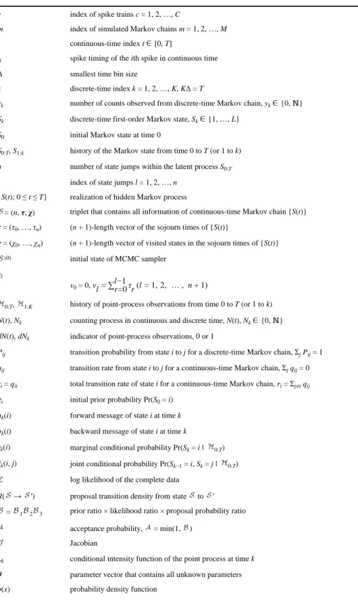
1.7 Notation
In neural spike analysis, we examine spike trains from either single or multiunit activity. Due to digitalized recordings, we assume that the time interval [0, T] of continuous-time neural spike train observations is properly discretized with a small time resolution Δ, so the time indexes are discrete integers within k ∈ [1, K], such that kΔ ∈ ((k − 1)Δ, kΔ] and KΔ = T. Let
denote the counting process for spike train c at time tk, and let denote the
indicator variable for 0/1 observation: if there is a spike and 0 otherwise. Other notations are rather straightforward, and we will define them in the proper places. Most notations used in this article are summarized in Table 1.
2 Discrete-Time Markov Modulated Probabilistic State-Space Model
To infer the neuronal UP and DOWN states, in this section we develop a simple, discrete-time Markov modulated state-space model that can be viewed as a variant of the standard HMM applied to spike train analysis. The underlying probabilistic structure is Markovian and homogeneous, and the inference algorithm is efficient in identifying the statistics of the hidden state process. Based on that, in the next section we develop a continuous-time probabilistic model in order to overcome some of limitations imposed by this discrete-time probabilistic model.
2.1 Hidden Markov Model
Let us consider a discrete-time homogeneous Markov chain. By discrete time, we assume that the time is evenly discretized into fixed-length intervals, which have time indices k = 1, …, K. The neuronal UP or DOWN state, which is characterized by a latent discrete-time first-order Markov chain, is unobserved (and therefore hidden), and the observed spike trains or the spike counts recorded from the MUA are functionally determined by the hidden state. The standard HMM is characterized by three elements: transition probability, emission probability,4 and initial state probability (Rabiner, 1989). At the first approximation, we assume that the underlying latent process follows a two-state HMM with stationary transition and emission probabilities.
• The initial probability of state is denoted by a vector π = {πi}, where πi = Pr(S0 = i) (i = 0, 1). Without loss of generality, we assume that the amplitude of the hidden state is predefined, and the discrete variable Sk ∈ {0, 1} indicates either a DOWN (0) or
UP (1) state.
• The transition probability matrix is written as
(2.1)
4The term emission probability arose from the HMM literature in the context of speech recognition; it refers to the probability of observing a (finite) symbol given a hidden state (finite alphabet).
NIH-PA Author Manuscript
NIH-PA Author Manuscript
with P01 = 1 − P00 and P10 = 1 − P11 corresponding to the transition probabilities from state 0 to state 1 and from state 1 to state 0, respectively.
• Given the discrete hidden state Sk, the observed numbers of total spikes across all
tetrodes (i.e., MUA), y1, y2, …, yK (yk ∈ ℕ), follow probability distributions that
depend on the time-varying rate λk,
(2.2)
where the parameter λk is determined by
(2.3)
where exp(μ) denotes the baseline firing rate and Sk denotes the hidden discrete-state
variable at time k. The term Nk−1 − Nk−J represents the total number of spikes observed
during the history period (k − J, k − 1], which accounts for the history dependence of neuronal firing. The choice of the length of history dependence is often determined empirically based on the preliminary data analysis, such as the histogram of the interspike interval (ISI). Equations 2.2 and 2.3 can be understood in terms of a generalized linear model (GLM) (e.g., McCullagh & Nelder, 1989; Truccolo, Eden, Fellow, Donoghue, & Brown, 2005), where the link function is a log function and the distribution is Poisson. Note that when β = 0 (i.e., history independence is assumed), we obtain an inhomogeneous Poisson process, and λk reduces to a Poisson rate
parameter.
Taking the logarithm to both sides of equation 2.2, equation 2.3 can be rewritten as
(2.4)
where ñk = Nk−1 − Nk−J. More generally, we can split the time period (k − J, k − 1] into several
windows (say, with equal duration δ), and equation 2.4 can be rewritten as
(2.5)
where β = {βj} and ñk = {ñk, j} are two vectors with proper dimensionality, and ñk, j = Nk−jδ −
Nk−(j+1)δ denotes the observed number of multiunit spike counts within the time interval (k −
(j + 1)δ, k − jδ]. If we further assume that the observations yk at different time indices k are
mutually independent, the observed data likelihood is given by
(2.6)
NIH-PA Author Manuscript
NIH-PA Author Manuscript
data, {yk} as the observed (incomplete) data, and their combination {Sk, yk} as the complete
data. Let θ denote all of the unknown parameters; then the complete data likelihood is given by
(2.7)
And the complete data log likelihood, denoted as , is derived as (by ignoring the constant)
(2.8)
where ξk(i, j) = Pr(Sk−1 = i, Sk = j).
2.2 Forward-Backward and Viterbi Algorithms
The inference and learning procedure for the standard HMM is given by an efficient estimation procedure known as the EM algorithm, which is also known as the Baum-Welch algorithm (Baum et al., 1970; Baum, 1972). Rooted in maximum likelihood estimation, the EM algorithm iteratively and monotonically maximizes (or increases) the log-likelihood function given the incomplete data (Dempster et al., 1977). In the E-step, a forward-backward procedure is used to recursively estimate the hidden state posterior probability. In the M-step, based on the missing state statistics (estimated from the E-step), the reestimation procedure and Newton-Ralphson algorithm are used to estimate the unknown parameters θ = (π, P, μ, α, β). In each full iteration, the EM algorithm iteratively maximizes the so-called Q-function,
(2.9)
the new θnew is obtained by maximizing the incomplete data likelihood conditional on the old parameters θold; and the iterative optimization procedure continues until the algorithm ultimately converges to a local maximum or a stationary point. For the self-containing purpose, we present a brief derivation of the EM algorithm (Rabiner, 1989) for the two-state HMM estimation problem.
2.2.1 E-Step: Forward-Backward Algorithm—In the E-step, the major task of the
forward-backward procedure is to compute the conditional state probabilities for the two states:
(2.10)
NIH-PA Author Manuscript
NIH-PA Author Manuscript
(2.11)
as well as the conditional state joint probability:
(2.12)
To make the notation simple, in the derivation below, we let the conditional θ be implicit in the equation.
To estimate equations 2.10 and 2.11, we first factorize the joint probability as
(2.13)
where
and the forward and backward messages ak(l) and bk(l) can be computed recursively along the
discrete-time index k (Rabiner, 1989):
where Pil denotes the transition probability from state i to l.
Given {ak, bk}, we can estimate equation 2.12 by
(2.14)
Furthermore, we can compute the observed likelihood (of the incomplete data) by
NIH-PA Author Manuscript
NIH-PA Author Manuscript
(2.15)
Given equations 2.13 and 2.15, the state posterior conditional probability is given by Bayes' rule,
(2.16)
In the term of the computational overhead for the above-described two-state HMM, the forward-backward procedure requires a linear order of computational complexity (4K) and memory storage (2K).
2.2.2 M-Step: Reestimation and Newton-Ralphson Algorithm—In the M-step, we
update the unknown parameters (based on their previous estimates) by setting the partial
derivatives of the Q-function to zeros: , from which we may derive either closed-form or iterative solutions.
Let ξk(i, j) = Pr(Sk−1 = i, Sk = j ∣ y1:K, θ) and γk(i) = Pr(Sk = i ∣ y1:K, θ) denote, respectively, the
conditional marginal and joint state probabilities (which are the sufficient statistics for the complete data log likelihood 2.9). From the E-step, we may obtain
(2.17)
The transition probabilities are given by Baum's reestimation procedure:
(2.18)
Specifically the transition probabilities P01 and P10 are estimated by closed-form expressions,
(2.19)
(2.20)
NIH-PA Author Manuscript
NIH-PA Author Manuscript
Next, we need to estimate the other unknown parameters (μ, α, β) that appear in the likelihood model. Since there is no closed-form solution for μ, α, and β, we may use the iterative optimization methods, such as the Newton-Ralphson algorithm or the iterative weighted least squares (IWLS) algorithm (e.g., Pawitan, 2001), to optimize the parameters in the M-step.
Let denote the computed mean statistic of a hidden state at time k; by setting the derivatives of with regard to the parameters α, μ, and β (and similarly for vector β), to zeros, we obtain
(2.21)
(2.22)
(2.23)
respectively. Typically, a fixed number of iterations is preset for the Newton-Ralphson algorithm in the internal loop within the M-step.
Finally, the convergence of the EM algorithm is monitored by the incremental changes of the log likelihood as well as the parameters. If the absolute value of the change is smaller than 10−5, the EM algorithm is terminated.
2.2.3 Viterbi Algorithm—Upon estimating parameters θ = (π, P, μ, α, β), we can run the
Viterbi algorithm (Viterbi, 1967; Forney, 1973) for decoding the most likely state sequences. The Viterbi algorithm is a dynamical programming method (Bellman, 1957) that uses the “Viterbi path” to discover the single most likely explanation for the observations. Specifically, the maximum a posteriori (MAP) state estimate Ŝk at time k is
(2.24)
The computational overhead of the forward Viterbi algorithm has an overall time complexity (4K) and space complexity (2K).
3 Continuous-Time Markovian and Semi-Markovian State-Space Models
The discrete-time probabilistic model discussed in the previous section imposes strong assumptions on the transition between the UP and DOWN states. First, it is stationary in the sense that the transition probability is time invariant; second, the transition is strictly Markovian. In this section, we relax these assumptions and further develop continuous-time, data-driven (either Markovian or semi-Markovian) state-space models, which is more
NIH-PA Author Manuscript
NIH-PA Author Manuscript
from the discrete-time model (developed in section 2) as the initialization condition, which also helps to accelerate the algorithmic convergence process.
3.1 Continuous-Time Probabilistic Model
One important distinction between the discrete-time and continuous-time Markov chains is that the former allows state changes to occur only at regularly spaced intervals, whereas the latter is aperiodic, in that the time between state changes is exponentially distributed. Therefore, the notion of a “single-step transition probability” is no longer valid in continuous time since the “step” does not exist. In fact, the transition probability in continuous time is characterized by either the transition rate or the sojourn time probability density function (pdf) between the two state change events. Let us assume that the pdf of the sojourn time for state j characterized by a parameter vector θj. Hence, the transition probability between state 0 (DOWN) and 1 (UP)
is characterized by the corresponding pdfs p(θ0, z) and p(θ1, z), respectively, where z is now the random variable in terms of holding time. For example, given the current state status (say, state j) and current time t, the probability of escaping or changing the current state (to other different state) will be computed from the cumulative distribution function (cdf):
(3.1)
and the probability of remaining in the present state will be computed from
(3.2)
which is known as the survival function in reliability and survival analysis. As seen, the transition probability matrix in continuous time now depends on the elapsed time (starting from the state onset) as well as the present state status. In general, we write the transition probability matrix as a parameterized form P(θ), where θ = (θ0, θ1) characterizes the associated sojourn time pdf parameters for the DOWN (0) and UP (1) states. As we will see, choosing different probability density models for the sojourn time results in different formulations of the continuous-time Markov or semi-Markov chain.
In modeling the neural spike train point processes, the CIF characterizes the instantaneous firing probability of a discrete event (i.e., spike). Specifically, the product between the CIF λ (t) and the time interval Δ tells approximately the probability of observing a spike within the interval [t, t + Δ) (e.g., Brown et al., 2003):
For each spike train, we model the CIF in a parametric form,5
5Here we assume that the individual CIF λc(t) can be modeled as a GLM with log(·) as a link function (Truccolo et al., 2005; Paninski, Pillow, & Lewi, 2007). One can also use other functions as the link function candidate, such as log(1 + exp(·)) or the sigmoidal (bell-shaped) function, whichever better reflects the neuron's firing properties (e.g., Paninski, 2004). The choice of the functional form for the CIF does not affect the inference principle or procedure described below.
NIH-PA Author Manuscript
NIH-PA Author Manuscript
(3.3)
where exp(μc) denotes the baseline firing rate for the cth spike train and βc denotes an
exponential decaying parameter that takes into account the history dependence of firing from time 0 upto time t. The nonnegative term defines a convolution between the exponential decaying window and the firing history of spike train c up to time t. Because of digitalized recording devices, all continuous-time signals are sampled and recorded in digital format with a very high sampling rate (32 kHz in our setup). Therefore, we still deal with the “discretized” version of a continuous-time signal. In this case, we sometimes use St and Sk
interchangeably if no confusion occurs. However, as we see below, their technical treatments are rather different. In the context of continuous-time observations (Δ = 1 ms), every time interval has at most one spike from each spike train. For computational ease, we approximate the integral in equation 3.3 with a finite discrete sum of firing history as follows:
(3.4)
where ñk is a vector containing the number of spike counts within the past intervals, and the
length of the vector defines a finite number of windows of spiking history. By assuming that the spike trains are mutually independent, the observed data likelihood is given by (Brillinger, 1988; Brown et al., 2003)
(3.5)
The complete statistics of the continuous-time latent process may be characterized by a triplet: = (n, τ, χ), where τ = (τ0, τ1, …, τn) is a vector that contains the duration lengths of sojourn times of , and χ = (χ0, χ1, …, χn) represents the states visited in these sojourns. Let ν0 = 0,
and νn+1 = T. Alternatively, the complete data likelihood, equation
3.5, can be rewritten in another form,
(3.6)
where denotes all of spike train observations during the sojourn time [νl−1, νl] for the
continuous-time (semi-)Markov process {S(t)}.
If we model each spike train as an inhomogeneous Poisson process with time-varying CIF λc(t), the expected number of spike counts observed within the duration [ν
l−1, νl] in the cth
spike train is given by the integrated intensity (also referred to as cumulative hazard function):
(3.7)
NIH-PA Author Manuscript
NIH-PA Author Manuscript
where denotes the spike counts of the cth spike train during the interval (νl−1, νl], and ti
denotes the continuous-time index of the ith spike of a specific spike train during the interval (νl−1, νl].
Ultimately, we can write the complete-data log likelihood in a compact form:6
(3.8)
where θj denotes the parameter(s) of the probability model of the sojourn time associated with
state j.
3.2 Continuous-Time Markov Chain
In a continuous-time Markov chain (i.e., Markov process), state transitions from one state to another can occur at any instant of time. Due to the Markov property, the time that the system spends in any given state is memoryless, and the distribution of the survival time depends on the state (but not on the time already spent in the state); in other words, the sojourn time is exponentially distributed,7 which can be characterized by a single rate parameter. The rate parameter, also known as the continuous-time state transition rate, defines the probability per time unit that the system makes a transition from one state to the other during an infinitesimal time interval:
(3.9)
The total transition rate of state i satisfies the rate balance condition:
(3.10)
6In addition to the compact representation, another main reason for this reformulation is the efficiency and stability of numerical computation in calculating the observed data likelihood or likelihood ratio.
7The exponential distribution with mean 1/λ is the maximum entropy distribution among all continuous distributions with nonnegative support that have a mean 1/λ.
NIH-PA Author Manuscript
NIH-PA Author Manuscript
The holding time of the sojourn for state i follows an exponential distribution exp(−riτ), or,
equivalently, the transition times of state i are generated by a homogeneous Poisson process characterized by rate parameter ri. For a two-state Markov chain, the transition rate matrix may
be written as
(3.11)
For an exponential random variable z, its cdf is computed as , where re−rz is the pdf of the exponential distribution with a rate parameter r. The reciprocal of the rate parameter, 1/r, is sometimes called the survival parameter in the sense that the exponential random variable z that survives the duration of time has the mean [z] = 1/r. In light of equations 3.1 and 3.2, at a given specific time t, the probability of remaining within the current state sojourn is . Let r0 and r1 denote the transition rate for states 0 and 1, respectively. Let τ = t − ν denote the elapsed time from the state transition up to the current time instant t; then the parameterized transition probability P = {Pij} is characterized by
(3.12)
Now, the transition probability, instead of being constant, is a probabilistic function of the time after the Markov process makes a transition to or from a given state (the holding time from the last transition or the survival time to the next transition).
3.2.1 Imposing Physiological Constraints—Due to biophysical or physiological
constraints, the sojourn time for a specific state might be subject to a certain range constraint, reflected in terms of the pdf. Without loss of generality, let p(τ) denote the standard pdf for a random variable τ, and let p̃(τ) denote the “censored” version of p(τ),8 which is defined by
where (·) is an indicator function and a > 0 and b ∈ (a, ∞) are the lower and upper bounds of the constrained random variable τ (which is always positive for the duration of the sojourn time), respectively. The scalar c is a normalized constant determined by c = F (b) − F (a), where F (·) denotes the corresponding cdf of the standard pdf p(τ) and F (∞) = 1. Likewise, the censored version of the cdf is computed by .
Suppose the sojourn time τ of a continuous-time Markov chain follows a censored version of the exponential distribution; then we can write its censored pdf as
8Censoring is a term used in statistics that refers to the condition that the value of an observation is partially known or the condition that a value occurs outside the range of measuring tool.
NIH-PA Author Manuscript
NIH-PA Author Manuscript
(3.13)
where the normalizing constant is given by c = F(∞) − F(a) = 1 − [1 − exp(−ra)] = exp(−ra).
3.3 Continuous-Time Semi-Markov Chain
In contrast to the Markov process, the semi-Markov process is a continuous-time stochastic process {St} that draws the sojourn time {νl} spent in specific discrete states from a
nonexponential distribution. In other words, the characterization of the sojourn time is no longer an exponential pdf. Table 2 lists a few examples of continuous-time probability models for characterizing the sojourn time duration for the interevent interval (Tuckwell, 1989). In general, the nonexponential censored pdf with a lower bound gives the flexibility to model the “refractory period” of the UP or DOWN state.
3.3.1 Two-Parameter Exponential Family of Distributions for the UP and DOWN State—To characterize the nonexponential survival time behavior of semi-Markov processes,
here we restrict our attention to three probability distributions that belong to the two-parameter exponential family of continuous probability distributions. We define the censored versions of three pdfs as follows:
• The censored gamma distribution p̃(τ; s, κ):
where κ and s represent the scale and shape parameters, respectively. If s is an integer, then the gamma distribution represents the sum of s exponentially distributed random variables, each with a mean κ. Similarly, c is a normalized constant for the censored pdf p̃(τ; s, κ): c = F(b) − F (a), and F (·) is the cdf of the standard gamma distribution.
• The censored log-normal distribution p̃(τ; μ, σ):
where the mean, median, and variance of the log-normal distribution are exp(μ + σ2/2), exp(μ), and exp(2μ + σ2)[exp(σ2) − 1], respectively.
• The censored inverse gaussian distribution p̃(τ; μ, s):
where μ and s represent the mean and shape parameters, respectively.
The choice of the last two probability distributions is mainly motivated by the empirical data analysis published earlier (Ji & Wilson, 2007). Typically, for a specific data set, a smoothed histogram analysis is conducted to visualize the shape of the distribution, and the
Kolmogorov-NIH-PA Author Manuscript
NIH-PA Author Manuscript
Smirnov (KS) test can be used to empirically evaluate the fit of specific probability distributions. Mostly likely, none of parametric probability distribution candidate would fit perfectly (i.e., within 95% confidence interval) for the real-world data; we often choose the one that has the best fit.9 In the simulation data shown in Figure 1, we have used the following constraints for the UP and DOWN states: [0.1, 3] (unit: second) for UP state and [0.05, 1] (unit: second) for DOWN state. The lower and upper bounds of these constraints are chosen in light of the results reported from Ji and Wilson (2007). Note that the shapes of the log-normal and inverse gaussian pdfs and cdfs are very similar, except that inverse gaussian distribution is slightly sharper when the value of the random variable is small (Takagi, Kumagai, Matsunaga, & Kusaka, 1997). In addition, the tail behavior of these two distributions differs; however, provided we consider only their censored versions (with finite duration range), the tail behavior is not a major concern here.
3.4 EM Algorithm
In the continuous-time model, we treat the individual spike trains separately and aim to estimate
their own parameters. Let denote the unknown
parameters of interest, where θup and θdown represent the parameters associated with the
parametric pdfs of the UP and DOWN states, respectively; the rest of the parameters are associated with the CIF model for respective spike trains. For an unknown continuous-time latent process {S(t); 0 ≤ t ≤ T} (where S(t) ∈ {0, 1}), let n be the number of jumps between two distinct discrete states. Let = (n, τ, χ) be a triplet of the Markov or semi-Markov process, where τ = (τ0, τ1, …, τn) is a vector that contains the duration of the sojourn time of and χ =
(χ0, χ1, …, χn) represents the states visited in these sojourns.
Let denote all the spiking timing information of the observed spike trains. Similar to the discrete-time HMM, we aim to maximize the Q-function, defined as follows:
(3.14)
The inference can be tackled in a similar fashion by the EM algorithm.
First, let us consider a simpler task where the transition time of the latent process is known and the number of state jumps is given. In other words, the parameters n and τ are both available, so the estimation goal becomes less demanding. We need to estimate only χ and θ.
Since the number of state transition, n, is known, p( , ∣ θ) is simplified to
(3.15)
Let ξl(i, j) = Pr( (χl−1) = i, (χl) = j) and γl(i) = Pr( (χl) = i). In the case of the
continuous-time Markov chain, the complete data log likelihood is given by
9Alternatively, one can use a discrete nonparametric probability model for the sojourn time, which is discussed in section 5.
NIH-PA Author Manuscript
NIH-PA Author Manuscript
(3.16)
where θ = (r0, r1, μ1α1, β1, …, μC, αC, βC) denotes the augmented parameter vector that contains
all of the unknown parameters. In the case of the continuous-time semi-Markov chain where the sojourn time is modeled by a nonexponential probability distribution, we can write the log-likelihood function as
(3.17)
where F (·) denotes the cdf of the nonexponential probability distribution.
Conditioned on the parameter θ, the posterior probabilities ξl and γl (for l = 1, …, n) can be
similarly estimated by the forward-backward algorithm as in the E-step for the HMM, whereas in the M-step, the new parameter θnew is obtained by
(3.18)
More specifically, for the parameters associated with the transition probability density model, we might, for example, assume that the UP and DOWN state durations are both log normal distributed with parameters θj = {μj, σj}(j = 0, 1), and they can be estimated by
(3.19)
In light of Table 2, setting the derivatives of μj and σj to zeros yields
where we have used in light of Table 2. The above two equations can be solved iteratively with the Newton-Ralphson algorithm.
NIH-PA Author Manuscript
NIH-PA Author Manuscript
Once the state estimate Ŝ(t) is available from the E-step,10 the parameters associated with the likelihood model can also be estimated by the Newton-Ralphson or the IWLS algorithm,
(3.20)
where λc(t) and are defined by equations 3.3 (or 3.4) and 3.7, respectively.
Notably, the EM algorithm described above has a few obvious drawbacks. Basically, it assumes that the information as to when and how many state transitions occur during the latent process is given; once the number of state jumps (say, n) is determined, it does not allow the number n to change, so it is incapable of online model selection. Furthermore, it is very likely that the EM algorithm suffers from the local maximum problem, especially if the initial conditions of the parameters are far from the true estimates. In the following, we present an alternative inference method to overcome these two drawbacks, and the method can be regarded as a generalization of the EM algorithm, except that the E-step state estimation is replaced by a Monte Carlo sampling procedure. This method is often called the Monte Carlo EM (MCEM) algorithm (Chan & Ledolter, 1995; McLachlan & Krishnan, 1996; Tanner, 1996; Stjernqvist, Rydén, Sköld, & Staaf, 2007). The essence of MCEM is the theory of Markov chain Monte Carlo (MCMC), which will be detailed below.
3.5 Monte Carlo EM Algorithm
The basic idea of MCMC sampler is to draw a large number of samples randomly from the posterior distribution and then obtain a sample-based numerical approximation of the posterior distribution. Unlike other Monte Carlo samplers (such as importance sampling and rejection sampling), the MCMC method is well suited for sampling from a complex and high-dimensional probability distribution. Instead of drawing independent samples from the posterior distribution directly, MCMC constructs a Markov chain such that its equilibrium will eventually approach the posterior distribution. The Markov chain theory states that given an arbitrary initial value, the chain will ultimately converge to the equilibrium point provided the chain is run sufficiently long. In practice, determining the convergence as well as the “burn-in time” for MCMC samplers requires diagnostic tools (see Gilks, Richardson, & Spiegelhalter, 1995, for general discussions of the MCMC methods). Depending on the specific problem, the MCMC method is typically computationally intensive, and the convergence process can be very slow. Nevertheless, here we focus on methodology development, and therefore the computational demand is not the main concern. Specifically, constructing problem-specific MCMC proposal distributions (densities) is the key to obtain an efficient MCMC sampler that has a fast convergence speed and a good mixing property (Brooks, Guidici, & Roberts, 2003). For the variable-dimension RJMCMC method, we present some detailed mathematical treatments in appendix A.
The Monte Carlo EM (MCEM) algorithm works just like an ordinary EM algorithm, except that in the E-step, the expectation operations (i.e., computation of sufficient statistics) are replaced by Monte Carlo simulations of the missing data. Specifically, M realizations of the latent process S(t) (0 ≤ t ≤ T) are simulated, and in this case the Q-function can be written as
10Note that Ŝ(t) is not the same as χl (l = 1, 2, …, n) in that the former is stochastic and the latter is deterministic.
NIH-PA Author Manuscript
NIH-PA Author Manuscript
(3.21)
where (m) denotes the mth simulated latent process for the unknown state (missing data). The M-step of MCEM is the same as the conventional M-step in the EM algorithm. Specifically, the parameters of the CIF appearing in the likelihood model are estimated using equation 3.20. However, the estimation of the parameters for the UP or DOWN state sojourn depends on the type of probability distribution. Here we distinguish three different possible scenarios. First, when the latent process is a continuous-time Markov chain and the sojourn time durations for the UP and DOWN states are both exponentially distributed, then θup and θdown correspond
to the rate parameters r1 and r0, respectively. The Q-function for a single Monte Carlo realization of can be written as
(3.22)
where nij denotes the number of jumps from state i to state j during [0, T], and
denote the total time or the sojourn length of {S(t)} spent in state i during [0, T]. Let denote the number of events that occur while {S(t)} is in state i; then it is known that the transition rate matrix can be estimated by q̂ij = nij/Ti and ri = qii = ni/
Ti, where nij, ni, and Ti are the sufficient statistics (Rydén, 1996). In this case, ri corresponds to the MLE. With M Monte Carlo realizations, the rate parameter will be estimated by
In the second scenario, when the latent process is a continuous-time semi-Markov chain where the sojourn time durations for both UP and DOWN states are nonexponentially distributed, the Q-function can be written as
(3.23)
where is obtained from the Monte Carlo mean statistic of M simulated latent processes. Similarly, the parameters of the nonexponential probability distributions can be estimated by their MLE based on their Monte Carlo realizations. For instance, in the case
NIH-PA Author Manuscript
NIH-PA Author Manuscript
of inverse gaussian distribution, the mean parameter is given by
, and the shape parameter is given by
. In the case of log-normal distribution, the
mean parameter is given by , and the SD parameter is
given by .
If, in the third scenario, one of the state sojourn time durations is exponentially distributed and the other is nonexponential, then the resulting latent process is still a semi-Markov chain, and the estimation procedure remains similar to that in the above two cases.
3.5.1 Initialization of the MCMC Sampler—It is important to choose sensible initial
values for the simulated (semi-) Markov chain since a poor choice of the initial (0) can lead to a sampler that takes a very long time to converge or result in a poor mixing of the (semi-) Markov chain. In our experiment, we typically use a discrete-time HMM model (with a 10 ms bin size) to estimate the hidden state sequence and then interpolate it to obtain an initial estimate of the continuous-time state process (with 1 ms bin size), from which we obtain the initial values of {n, τ, χ}.
3.5.2 Algorithmic Procedure—In summary, the MCEM algorithm is run as follows: • Initialize the MCMC sampler state for = {n, τ, ν}.
• Iterate the MCEM algorithm's E and M steps until the log likelihood reaches a local maximum or saddle point.
1. Monte Carlo E-step: Given an initial state (0), run the RJMCMC sampling procedure to draw M Monte Carlo samples , based on which to compute the necessary Monte Carlo sufficient statistics.
2. M-step: estimate the parameters {θup, θdown} with their MLE.
3. M-step: optimize the parameters according to equation 3.20. • Upon convergence, reconstruct the hidden state Ŝ(t) in the continuous-time domain.
• Compute λc(t) for each spike train c, and conduct goodness-of-fit tests (see below) for all spike trains being modeled.
3.5.3 Reconstruction of Hidden State—There are two ways to reconstruct the hidden
state of the latent process. The first is to apply the Viterbi algorithm once the MCEM inference is completed (when n and τ have been determined). In the second, and simpler, approach, we can determine the state by the following rule (Ball et al., 1999). For m = 1, 2, …, M, let
(3.24)
and let , and the point estimate of the hidden state is
NIH-PA Author Manuscript
NIH-PA Author Manuscript
(3.25)
Furthermore, the marginal prior probability of the hidden state is given by
(3.26)
3.5.4 Goodness-of-Fit Tests—Upon estimating the CIF model λc(t) for each spike train
(see equation 3.3), the goodness of fit of the estimated model is tested in light of the time-rescaling theorem (Brown, Barbieri, Ventura, Kass, & Frank, 2002). Specifically, given a point process specified by J discrete events: 0 < u1 < ⋯ < uJ < T, define the random variables
for j = 1, 2, …, J − 1. Then the random variables zjs are independent,
unit-mean exponentially distributed. By introducing the variable of transformation vj = 1 − exp
(−zj), vjs are independent and uniformly distributed within the region [0, 1]. Let gj = Φ−1(vj)
(where Φ(·) denotes the cdf of the standard gaussian distribution); then gjs will be independent
standard gaussian random variables. Furthermore, the standard Kolmogorov-Smirnov (KS) test is used to compare the cdf of vj against that of the random variables uniformly distributed
within [0, 1]. The KS statistic is the maximum deviation of the empirical cdf from the uniform cdf. To compute it, the vjs are sorted from the smallest to the largest value; then we plot values
of the cdf of the uniform density defined as against the ordered vj s. The points should
lie on the 45 degree line. In a Cartesian plot of the empirical cdf as the y-coordinate versus the
uniform cdf as the x-coordinate, the 95% confidence interval lines are . The KS distance, defined as the maximum distance between the KS plot and the 45 degree line, is used to measure the lack of fit between the model and the data.
Furthermore, we measure the independence of the time-rescaled time series by computing the
autocorrelation function of gjs: . Since gjs are normally
distributed, if they are independent, then they are also uncorrelated; hence, ACF(m) shall be
small for all values of m, and the associated 95% confidence interval is .
3.5.5 Implementation and Convergence—Let the triple = (n, τ, χ) denote all the
information of the continuous-time latent process, which contains n state jumps and n + 1 durations of corresponding sojourn times, and the discrete states that are visited in the sojourns. To simulate the Markov chain, we first obtain the initial conditions for both the state and parameters { (0), θ(0)}. Next, we run the MCMC sampler (see appendix A for details) to generate a sequence of Monte Carlo samplers { (k)} for k = 1, 2, …, M, and the realizations { (k)} can be viewed as the samples drawn from the conditional posterior p( ∣ , θ). At each MCEM step, the parameter vector θ is updated in the Monte Carlo M-step using the sufficient statistics obtained from p( ∣ , θ). Typically, to reduce the correlation of the simulated samples, a “burn-in” period is discarded at the beginning of the simulated (semi-) Markov chain. Even after the burn-in period, the successive realizations of { (k)} might still be highly
NIH-PA Author Manuscript
NIH-PA Author Manuscript
correlated. This problem can be alleviated by using the “thinning” or subsampling technique: every Np simulated samples in the chain is used. Although the thinning technique can increase
the Monte Carlo variance of the estimate (Geyer, 1992), it is widely used in practice to reduce the correlation among the samples. In our experiment, we typically chose Np = 10.
At the end of each Monte Carlo sampling step, the sufficient statistics for computing the acceptance probability and updating the parameter θ (in the M-step) need to be stored, and all new information (n, τ, χ) needs to be updated each time changes.
In terms of convergence, Markov chain theory tells us that when M → ∞, the samples are asymptotically drawn from the desired target (equilibrium) distribution. However, choosing the proper value of M is often problem dependent, and the convergence diagnosis of the MCMC sampler remains an active research topic in the literature (e.g., Gelman & Rubin, 1992; Cowles & Carlin, 1996).
4 Experimental Results
4.1 Synthetic Data
First, we simulate four spike trains with the time-rescaling theorem (see Figure 2 for a snapshot of one realization). The latent state variable is assumed to be drawn from a two-state discrete space: S(t) ∈ {0, 1}. The simulation is conducted with a 1 ms time bin size with the following model:
where ñ(t) denotes the number of spike counts across all spike trains during the previous 100 ms prior to the current time index t, and the parameters of individual spike trains are set as follows:
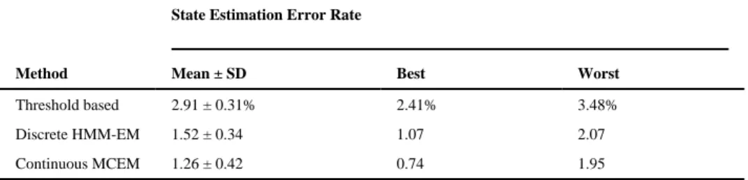
For the simulated hidden latent process, the total duration is T = 30 s, and the number of jumps varies from 35 to 45, yielding an average occurrence rate of state transitions of about 80 min−1. Furthermore, we assume that the sojourn time durations for both UP and DOWN states follow a log-normal distribution. For the UP state, the survival time length is randomly drawn from logn(−0.4005, 0.8481) (such that the mean and median value of the duration are 0.67 s and 0.96 s, respectively), with a lower bound of 0.15 s; and for the DOWN state, the survival time length is randomly drawn from logn(−1.9661, 0.6231) (such that the mean and median value of the duration are 0.14 s and 0.17 s, respectively), with a lower bound of 0.05 s. To test the discrete-time HMM model, the spike trains are binned in 10 ms and collected by spike counts. We employed the EM algorithm with the following initialization parameters: π0 = π1 = 0.5, P00 = P11 = 0.9, P01 = P10 = 0.1. For the synthetic data, the EM algorithm typically converges within 200 iterations. The forward-backward algorithm computes all necessary sufficient statistics. Upon convergence, the Viterbi algorithm produced the ultimate state sequence output, yielding an average decoding error rate of 1.52% (averaged over 10 independent runs). In this case, since the CIF model is given (no model mismatch issue is involved), the decoding error rate is reasonably low even with the discrete-time HMM. As a
NIH-PA Author Manuscript
NIH-PA Author Manuscript
It was found (see Table 3) that the discrete-time HMM method yields better performance than the threshold-based method. Figure 3 plots a snapshot of hidden state estimation obtained from the discrete-time HMM in our experiments.
Next, we applied the MCEM algorithm to refine the latent state estimation in the continuous-time domain. Naturally, with a smaller bin size, the continuous-continuous-time model allows precisely segmenting the UP and DOWN states for identifying the location of state transition. With the initial conditions obtained from the discrete-time EM algorithm, we simulated the Markov chains for 20,000 iterations and discarded the first 1000 iterations (“burn-in” period). For the synthetic data, the MCEM algorithm converged after 20 to 30 iterations, and we were able to further improve the decoding accuracy by reducing the average error rate to 1.26%. As seen in Table 3, the continuous-time model outperformed the discrete-time HMM model in terms of the lower estimation error. However, in terms of estimating the correct number of state transitions, the HMM obtained nearly 100% accuracy in all 10 Monte Carlo trials (except for two trials that miscount two more jumps); in this sense, the HMM estimation result can be treated as a very good initial state as the input to the continuous-time semi-Markov chain model. In addition, the continuous-time model yields a 10 times greater information transmission rate (1 bit/ms) than the discrete-time model (1 bit/10 ms). We also computed the probability distribution statistics of the UP and DOWN states from both estimation methods. In the discrete-time HMM, we used the sample statistics of the UP and DOWN state durations as the estimated results. These results were also used as the initial values for the continuous-time semi-Markov process, where the MCEM algorithm was run to obtain the final estimate. The results are summarized in Table 4.
Once the estimates of {S(t)} and {μc, αc, βc} become available, we compute λc(t) for the
simulated spike trains in continuous time (with Δ = 1 ms). Furthermore, the goodness-of-fit tests are employed to the rescaled time series, and the KS plots and the autocorrelation plots for the simulated spike trains are shown in Figure 4. As seen from the figure, these plots fall almost within the 95% confidence bounds, indicating the model fit is sufficiently satisfactory. Finally we also do extra simulation studies by examining the sensitivity of different methods regarding the change of two factors: the modulation gains of the hidden state and the number of observed spike trains. The first issue examines the impact of the global network activity during the UP state, that is, the αc component appearing in λc(t). Specifically, we modify the
gain parameters of individual spike trains (while keeping remaining parameters unchanged) as follows:
such that each λc is reduced about 20% during the UP state period. It appears that the average
performance of the threshold-based method degraded from the original 2.91% to 3.62% (with a trial-and-error selected threshold), while the performance of the probabilistic models remained almost unchanged. This is partly because of the fact that a correct generative model is used and the uncertainties of the hidden state were taken into account during the final estimation (see Figure 5). In the meantime, if αc is decreased more and more, the mean MUA
firing rate will be significantly decreased, the rate difference between UP and DOWN periods is reduced, and therefore the ambiguity between them increases. At some point, it can be imagined that all methods will break down unless the bin size is increased accordingly (at the cost of loss of accuracy in the classification boundary). Due to space limitations, we do not explore this issue further here.
NIH-PA Author Manuscript
NIH-PA Author Manuscript
The second issue examines the estimation accuracy of the missing variable against the number of observed variables. It is expected that as more and more observations are added, the resulting discrepancy between the threshold-based method and the probabilistic models will also become smaller, since the uncertainty of the hidden state is less (or the posterior of the hidden variable is larger with more spike train observations). In our simulations, we did extra experiments by either reducing or increasing the number of simulated spike trains, followed by rechecking the results across different setups for different methods. The estimation error results are
summarized in Figure 6. Specifically, for the threshold-based method, as more and more spike trains are added, its estimation error gradually improves. This is expected since the threshold selection criterion (see appendix B) heavily depends on the number of the spike train observations, and adding more spike train observations help to disambiguate the boundary between the UP and DOWN states. Meanwhile, for the probabilistic models, the estimation performance either slightly improves (in the discrete-time HMM) or remains roughly the same (in the continuous-time model). This is partly because adding more observations will also increase the number of parameters to be estimated in the continuous-time model, so the difficulty of inference also increases; whereas the HMM performance is likely to saturate quickly due to either the insufficiency of the model or the local minimum problem inherent in the EM algorithm. This observation implies that the probabilistic models are particularly valuable when the number of spike train observations is relatively small and that the simple threshold-based method becomes more and more reliable in terms of estimation accuracy— yet its performance is still worse than that of two probabilistic models. This is probably because it is difficult to find an optimal kernel smoothing parameter or the two threshold values (see appendix B). Moreover, the threshold-based method cannot produce the statistics of interest (e.g., posterior probability, transition probability).
4.2 Real-World Spike Train Data
Next, we apply our models to validate some real-world simultaneously recorded spike trains collected from one behaving rat (Vijayan, 2007), where the MUA, cortical and hippocampal EEGs, and EMG have been simultaneously recorded (see Figure 7 for a snapshot). We presented the spike train data of a single animal (in one day), recorded from the primary somatosensory cortex (SI) during SWS. Neurophysiological studies of neural spike trains and EEGs across different rats and different recording days, as well as the comparison between the cortex and hippocampus, will be presented elsewhere. In this study, 20 clearly identified cortical cells from eight tetrodes were recorded and sorted. All spiking activity from these eight tetrodes was used to determine the UP and DOWN states.
For this study, we selected about 15.7 minutes of recordings from a total of 11 (interrupted) SWS periods of one rat,11 where the mean ± SD length of SWS periods is 85.7 ± 35.8 s (maximum 156.1 s, minimum 30.7 s). We pulled out the multiunit spikes from eight tetrodes (no spike sorting is necessary here). For each spike train (from one tetrode), we empirically chose the following CIF model, as defined in the continuous-time domain:12
11The sleep stage classification was based on the recordings of electromyography (EMG) and hippocampal and cortical EEGs (ripple power, theta and delta power). SWS is characterized as having low EMG, high hippocampal ripple, low hippocampal theta (4–8 Hz), and high cortical delta (2–4 Hz). In practice, we varied the cut-off thresholds of those parameters (via grid search) to obtain a suboptimal SWS classification for a specific rat.
12The model was empirically verified by model selection based on the GLM fit of a small data set using the glmfit function in Matlab. The model with the lowest deviance (defined by twofold negative log likelihood) or the smallest Akaike's information criterion (AIC) value will be chosen.