Adaptive motor control using predictive neural networks

Adaptive Motor Control Using Predictive Neural

Networks

by

Fun) Wey

Submitted to the Department of Brain and Cognitive Sciences

in partial fulfillment of the requirements for the degree of

Doctor of Philosophy in Computational Neuroscience

at the

MASSACHUSETTS INSTITUTE OF TECHNOLOGY

September 1995

©

Fun Wey, MCMXCV. All rights reserved.

The author hereby grants to MIT permission to reproduce and

distribute publicly paper and electronic copies of this thesis

document in whole or in part, and to grant others the right to do so.

A

uthor

. ... ...

Department of Brain and Cognitive Sciences

September 7th, 1995

Certified by.... ... ... ... . .

..

..

...

Michael I. Jordan

Professor

Thesis Supervisor

Accepted

by ...

/. . a . . _.

.

ASACUTS INSTITUTE

Gerald

E. Schneider

..AS.rACHSETS INSTITUTE

Chairman, Departme'n'tk

i

tee on Graduate Students

SEP 12 1995

Adaptive Motor Control Using Predictive Neural Networks

by

Fun Wey

Submitted to the Departrent of Brain and Cognitive Sciences on September 7th, 1995, in partial fulfillment of the

requirements for the degree of

Doctor of Philosophy in Computational Neuroscience

Abstract

This thesis investigates the applicability of the forward modeling approach in adaptive motor control. The forward modeling approach advocates that in order to achieve effective motor control, the controller must first be able to predict the outcomes of its actions with an internal model of the system, which can be used in the search for the appropriate actions to achieve particular desired movement goals. In realistic control problems, however, the acquisition of a perfect internal dynamical model is not generally feasible. This thesis shows how an approximate forward model, obtained via a simple on-line adaptation algorithm and an on-line action-search process, is able to provide effective reaching movement control of a simulated three-dimensional, four-degree-of-freedom arm.

In the course of studying the on-line action search process, a problem which we refer to as the "control boundary problem' was identified. This problem was found to occur frequently and was found to be detrimental to the gradient-based search method. We developed a novel technique for solving the problem, referred to as the "moving-basin approach.' The moving basin approach leads the system to the desired goal by adaptively creating subgoals. Results are reported that show the improvement in the action-search process using the moving basin method.

Once the control boundary problem is solved, the forward modeling approach is able to provide stable adaptive control under perturbations of various forms and magnitudes, including those that could not be handled by analytical adaptive control methods. Further investigation also revealed that changes within the parameters of a forward model can provide information about the perturbed dynamics.

Thesis Supervisor: Michael I. Jordan Title: Professor

Acknowledgments

I am awfully short of words to fully express my gratitude towards Mike Jordan for all he has done for me throughout my study at MIT. Mike has been highly tolerant towards my incompetence and rebellious nature, and had gone through maneuvers around the department to maintain the well-being of my studentship. I will probably not be able to find another person with such a compassionate heart. In fact the most important lesson I learned from Mike is his patience and tolerance. In my future career as a leader of a research team, my experience with these important qualities will most certainly turn out to be extremely beneficial.

I would also like to thank the government of Singapore for having achieved the economic miracle for the Republic, by which my study at MIT became possible. I am from a poor family, and my parents would not have imagined that their son could one day attain a PhD degree from the world's most prestigious school of science and technology. My government has been very supportive of my study by providing me a precious scholarship that extensively covered my study at MIT. In particular, I would like to thank the Chief Defense Scientist for attending my thesis defense. This is a great honor for me.

I would like to thank the members of Jordan lab for their friendship, support and encouragement throughout these years. In particular, I would like to thank John Houde for correcting some parts of my thesis.

I would like to thank Janice Ellertsen for her graceful assistance and care through-out these years. She alleviated my workload by keeping a close watch on administra-tive requirement related to my study.

Finally I would like to thank all members of my thesis committee (Prof Ronald Williams, Prof Tomaso Poggio and Asst Prof Peter Dayan) for their kind comments on my thesis, and being so helpful and considerate in granting me the PhD degree.

Contents

1 Introduction

1.1 Background and Motivation ... 1.2 Organization of the thesis ...

2 Motor Dynamics and its Adaptive Control

2.1 Introduction.

2.2 Manipulator's Dynamics ...

2.3 A Glimpse of the Complexity involved in Motor Dynamics ... 2.4 Review of Adaptive Control Schemes for Manipulators

2.4.1 Craig's Adaptive Scheme .

2.4.2 Slotine's scheme .

3 Forward Modeling and On-line Adaptation

3.1 Introduction.

3.2 Distal supervised learning ...

16 16 19 21 21 22 23 . . . .. 25 26 28 30 30 30

3.3 Some Psychophysical Evidence of the existence of Forward Models 3.4 Forward modeling for Manipulator Control ...

3.4.1 Trajectory Planning.

3.4.2 Nature of mapping and Learning Efficacy ... 3.5 On-Line Adaptation ...

3.6 Control of a four degree-of-freedom arm in 3-D space ... 3.6.1 Forward model.

3.6.2 Controller ...

4 The Moving Basin Mechanism

4.1 Introduction.

4.2 The control boundary problem ... 4.3 The moving basin mechanism ...

4.3.1 Choosing the starting point . . 4.3.2 Stationary points ...

4.4 Simulation Results.

4.4.1 Performance within a trajectory 4.4.2 Global Performance ... 4.5 Discussion ... 33 34 35 36 37 42 42 44 45 45 46 50 51 52 53 53 53 56

5 Adaptive Control of a 4-dof arm 5.1 Introduction.

5.2 Robustness to Perturbed Dynamics ...

5.2.1 Performance with changes of the links' masses ... 5.2.2 Performance with errors in the joint angle sensors ... 5.2.3 Performance with errors in joint velocity sensors ... 5.3 Inter-Trajectory Performance.

5.4 Properties of the adapted network ... 5.4.1 Distributed changes .

5.4.2 "Shaking out" of perturbation information with white noise 5.4.3 Effect on global prediction accuracy ...

6 Performance Using Various Learning Architectures

6.1 Introduction.

6.2 Performance of neural networks ...

6.3 Performance of Local Expert networks ... 6.4 Performance of Hyper-Basis Functions.

6.5 Comparing to Craig's method ...

7 Conclusion 57 58 58 59 59 62 64 64 67 77

80

80 81 82 83 . .. 84

88

57

A Monotonicity, convexity and symmetry of direct-drive manipulator's

dynamics

B Utilizing logistic action nodes

90

List of Figures

2-1 a 2-joint revolute arm. ... ... 23

3-1 An inverse model as a feedforward controller. With the direct-inverse modeling technique, the inverse model will be trained to perform the map u[t] = f-l'(y[t + 1],x[t]), where y[t + 1] is the observed system's output caused by an action u[t] at state x[t] ... 31 3-2 The distal supervised learning approach. The forward model is trained

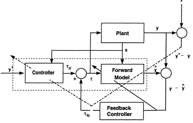
using the prediction error y[t] - [t]. The controller is trained by propagating the performance error y*[t] - y[t] backward through the forward model to yield an incremental adjustment to the controller. It is also possible to propagate the predicted performance error y*[t] - r[t] backward through the forward model. This can be done iteratively to find a locally optimal control signal based on the initial control signal proposed by the controller ... 32 3-3 Feedback controller to correct the error in feedforward torque ff via

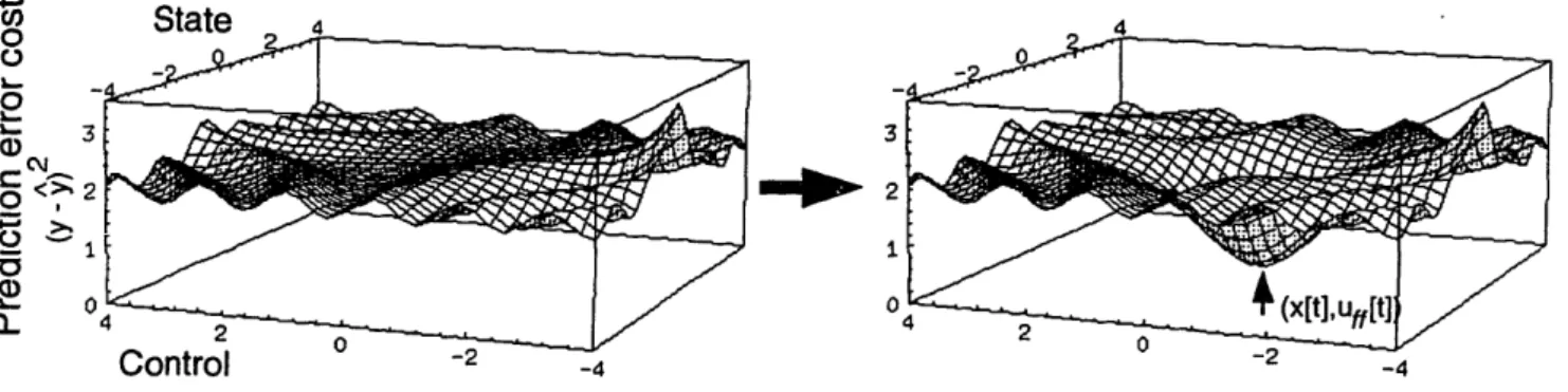
3-4 The local generalizing effect of on-line adaptation in the forward model of an single-state SISO system. The learning of an exemplar y[t + 1] =

f(x[t], uff[t]) at time step t + 1 leads to the reduction of prediction

error in a neighborhood of (x[t], uff[t]). . . . . 4 0

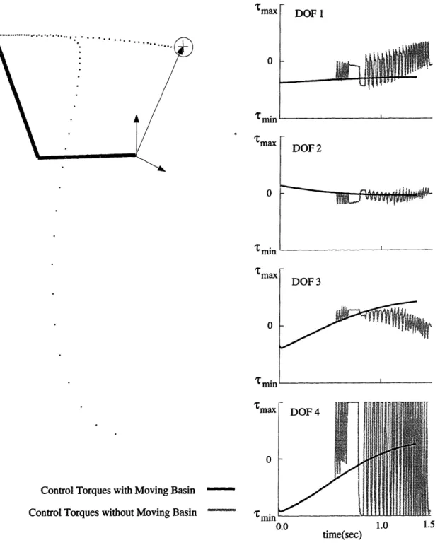
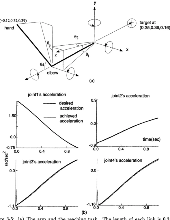
3-5 (a) The arm and the reaching task. The length of each link is 0.3 m. The center of mass of each link is at the center of the link. The maxi-mum torques at the shoulder are 91.3 N m, whereas those at elbow are 15.6 N m. The experiments on robustness involved a reaching move-ment from the point (-0.12, 0.32, 0.39) to the point (0.25, 0.36, 0.16).

The joint angles in the initial configuration were (01, 02, 03, 04) = (0.14, 0.24, 0.04, 1.04).

(b) Performance of the controller with nominal dynamics in the reach-ing task. Note that the scales of the graphs of each joint are not the same. The performance error at the beginning of the trajectory is 2.66 rad/s2. The target is reached in 1.05 seconds. ... 43

4-1 (a). The path {r(i)[t + 1]} taken by steepest descent is generally nonlin-ear and often reaches the boundary of the predicted achievable target set y. The moving basin mechanism tends to straighten the path, al-lowing the target to be reached. (b) A plot of the deviations of S(i)[t+1]

from the line joining Sr(°)[t + 1] and y*[t + 1] in an actual action-search process, with and without the use of moving basin mechanism. With a 4-step target-shift the deviation is reduced by approximately 83 percent. 48 4-2 The basin on the left corresponds to the cost J when

Vg

9[t + 1] is the

target, and the basin on the right corresponds to the cost J when

y*[t + 1] is the target. The basin of J is shifted by slowly shifting

the virtual target from jrg[t + 1] to y*[t + 1], and the action-search

finds the locally-optimal action u(i)[t] for each virtual target until the feedforward action uff [t] is found. Note that the state and the forward model's parameters are invariant during the search process ... 51

4-3 (a) Performance with and without the moving basin. The hand is able to reach the target with a fairly straight path with using the moving basin. Without the moving basin the control is able to track the desired trajectory up to _ 0.5sec, after which the control boundary problem occurs and the hand strays and exhausts one of its degrees of freedom. 54

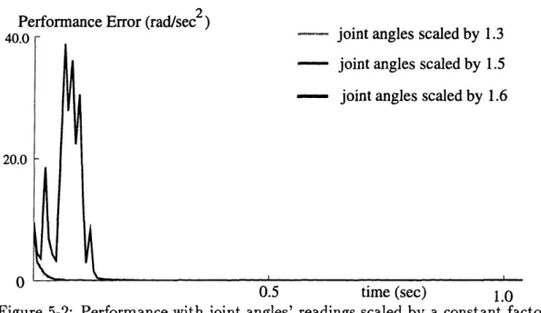
5-1 Performance with mass of link 1 changed by a constant factor. The target is reached within 1.3 seconds in all cases. ... 59 5-2 Performance with joint angles' readings scaled by a constant factor. . 60 5-3 Performance with joint angles' readings shifted by a constant amount. 60 5-4 Performance with joint velocity readings scaled by a constant factor.. 61 5-5 Performance with joint velocity readings shifted by a constant amount. 61 5-6 Performance for distinct trajectories under various perturbations. (a)

shows the average (in dark line) of the maximum performance errors encountered in each trajectory (in grey line) when the d.o.f.4's torque is increased threefold. (b) to (d) show the averages of the max perfor-mance errors under respective listed perturbations to the dynamics.. 63 5-7 The changes in the forward model after the arm has reached the target

in the reaching task. The density of a connecting line is proportional to the magnitude of change of the connection. The darkest line cor-responds to the maximum magnitude of weight change (lAwJlloo). (a) shows the changes under nominal dynamics. (b) shows the changes with scaling of linkl's mass by 5.0 (ref Figure 5-1). In both cases the IlAwoo is small compared to the original forward model's maximum

5-8 The changes in the forward model after the completion of the second reaching task. The density of a connecting line is proportional to the magnitude of change of the connection. The darkest line corresponds to the maximum magnitude of weight change (Awlloo). (a) shows the much-distributed changes with scaling of DOF4's torque by 3.0 only. The actual perturbation in the plant cannot be observed. (b) shows the changes with scaling of DOF4's torque by 3.0 and white noise at state input. The much larger changes at the connections proximal to DOF4's input indicates that the main problem is at DOF4's input. Note also that although JAwil increases by only 91% in (b), [Il\wII

increases by 455%. ... 66 5-9 The changes in the forward model after the completion of the second

reaching task with scaling of DOF4's torque by 3.0, white noise at state input and scaling of 91 by 35.0. In this case H(r4) = 8.82 and H(01) = 4.21, which are the highest and second highest of all Hs

respectively ... 76

5-10 Typical influence of the local adaptation in global prediction accuracy. (a) shows the improvement in global prediction at a distance of up to , 0.73 from (x', r') when performing under nominal dynamics. (b) the improvement at a distance of up to m 0.9 when performing with the scaling of joint angles by 1.6. (c) improvement at up to 1.05 when performing with the shifting of joint angles by 0.7 rad. (d) the improvement at up to ~ 1.2 with threefold increase of DOF4's torque. 79

6-1 In Craig's control scheme, parameters diverge when excitation is lack-ing. Adapted from Craig 1988 ... 86

6-2 Parameters in a HBF forward model slowly drifting away to a stable point due to noise present in the inputs, even when the arm is not moving. Note that the drifted amount is small compared to the squared length of the parameters: lwll = 21.15, while lAwll < 0.009 ... 87

List of Tables

6.1 Performance of two neural networks under nominal condition ... 6.2 Performance of NN under nominal and perturbed conditions... 6.3 Performance of LEN (with 4 local experts) under nominal and

per-turbed conditions ...

6.4 Performance of two HBF networks under nominal condition ... 6.5 Performance of HBF network under nominal and perturbed conditions 6.6 Performance using HBF under perturbed conditions with (w/ o-l) and

without (w/o o-l) online adaptation . ...

82 82 83 83 84 84

An Overview

This thesis work is prompted by the recent growth of research into the application of neural networks for the control of nonlinear systems. Specifically, it involves research into the applicability of the forward modeling idea in adaptive motor control.

The forward modelling approach to motor learning and control is an idea simi-lar to the indirect methods in the adaptive control literature. It advocates that in order to achieve adaptive motor control, the controller must first be able to predict the outcomes of its actions (given the state information of the environment) with a model of the system. This predictive capability should then be utilized in the search for the appropriate actions in a particular situation. The idea is conjugate to the direct methods which do not involve building a model of the dynamical system to be controlled.

The original forward modeling idea involves:

1. the off-line training of neural networks with large number of exemplars;

2. the performance of the neural networks during the applied stage with feedfor-ward computations only.

Most other connectionist architectures for adaptive control of nonlinear systems, in either direct or indirect form, require the neural networks to assume a role similar to that postulated above. There has not been any work on investigating the performance

of these architectures with the ANN's learning of a small number of on-line exemplars. This may be due to the fact that ANN training usually requires many exemplars and epochs to approximate a target function accurately, which created the presumption that the NN's learning of a small number of on-line exemplars will not do much.

The idea has been tested in the control of simulated robotic arms. In each simu-lation a neural network (forward model) was trained off-line to predict the resultant joint accelerations caused by torques applied to the joints at any given state of the arm. If this prediction is highly accurate, the sequence of feedforward torques re-trieved from the forward model (using the bac,;'propagation algorithm) would lead to the accurate execution of a desired trajectory (specified in the form of a sequence of desired joint accelerations). However an exact forward model of the dynamics of a robotic arm (even a simple one) produced by off-line training alone is not possible. There is thus a need to adapt on-line the forward model if the approach is to work without incorporating additional auxiliary controllers. A simple adaptation method is to train the forward model on each exemplar collected on-line (after the execu-tion of its acexecu-tion in each time-step of the control). In view of the large amount of exemplars and time taken to off-line train the forward model, I presumed that this one-exemplar-at-each-time-step learning will not work. To my surprise the forward model is able to stably adapt to various kinds of nonlinear perturbations (of high mag-nitudes) to the arm dynamics with this method, and in turn performs highly accurate trajectory tracking. Further investigation revealed that the structure of the forward model could provide information about what the perturbations are. It also provides impressive generalizing power such that the learning of a single exemplar could lead to improvement of prediction in a large neighborhood in the forward model's input space. This discovery leads to new research into the computational properties of neural networks in general, and in particular its applicability in adaptive control of nonlinear systems.

Chapter 1

Introduction

Whatever you can do, or dream you can do, begin it!

Boldness has genius, magic, and power in it.

Begin it now!

- Goethe

1.1 Background and Motivation

The urge to understand and better control our bodily movements has been around throughout the ages. During the warring years early in human history, a better knowledge of this field would yield better fighting forces, and this in turn could mean the dominance of a particular race or nation over its neighbors. With the advances of science and technology in modern era, we see the ongoing quest for intelligent robotics for better industrial production and military capabilities. The need to find treatments for illnesses related to human motor control, such as Parkinson and Huntington diseases, and design of actuator interfaces for the disabled, also require a better understanding of biological motor control systems.

Of the various motor faculties, arm movements have attracted the most attention among researchers. While it is known that the inherent dynamics of human arms are nonlinear and complex, we can effortlessly execute highly flexible and complex arm movements under many conditions. Research into the arms' motor control system has in recent years evolved into a multi-disciplinary field involving robotics, medical science, adaptive control theory, psychophysics and, recently, computational neuro-science, in the hope that breakthroughs could be achieved through the convergence of both engineering and reverse-engineering approaches.

The reverse-engineering approach, which consists of the search for control strate-gies adopted by nature by looking at the actual neural circuits in biological systems, quickly run aground because of the difficulty in linking the implementing circuits to the inherent dynamics involved. To date numerous models involving only the use of feedback control circuits (e.g. alpha-gamma coactivation - see Kandel & Schwarz 1991) to handle perturbed dynamics of the arms have been proposed; but such con-trol schemes can only explain how local improvement in movement concon-trol can be achieved. Since it is known that biological control systems are able to generalize from a small amount of experimenting with the perturbed dynamics of the motor faculties and lead to global improvement in performance, a framework that could fully model the competence of a biological motor system would have to be made within the realm of adaptive motor control.

The engineering approach mainly involves the modeling of the nominal dynamics of the arms using its artificial counterpart - i.e. the robotic manipulator with revolute joints, which can be achieved using numerous formulation strategies. Of these strate-gies, the most notable ones are the Newton-Euler formulation and the Lagrangian formulation, by which many formal adaptive methods for robotic manipulators have been established in recent years. The fast development of adaptive control for ma-nipulators, which is by itself a specialized field, is due to the fact that the effective control of robotic manipulators is inherently linked to industrial interests; and conse-quently they provide enormous support for such development. These adaptive control

methods, many of them well-established in handling certain specific domains of per-turbed dynamics, provide the theoretical framework that might be adapted to model the adaptive capabilities of biological motor systems. Such attempts would have to be made within the constraint of biological plausibility at the implementational level. In particular, effort would have to be made to tackle a challenging fact - the com-putational modules of biological motor systems consist of huge number of processing units, each limited in computational capabilities but whose global connectedness pro-vide powerful learning capabilities. Many such attempts were made in recent years (e.g. see Lewis 1995, Miller 1990), and it is this interface that this thesis work is aimed at.

There are core organizational principles at a conceptual level which provide con-straints narrowing our scope of research directions at this interface. For example, Jordan & Rumelhart (1992) have clearly argued that forward modeling is more likely to have been adapted by motor circuits as the control strategy for certain aspects. Such control methods involve an identification procedure in which the control system forms an approximate internal model of the system that is being controlled, coupled with a search process in which the model is used to search for control signals (also see Narendra & Parthasarathy, 1990). This leads to the concept of distal supervised learning in which the controller is trained using a model of the system to be controlled. The original forward modeling idea utilizes auxiliary feedback controllers to im-prove the performance of an inaccurate controller trained by an approximate forward model. The forward model and controller can then be re-trained off-line with the exemplars collected to yield better feedforward control. The core idea in this thesis stretches the approach a bit further - the feedback controller is discarded altogether so that there is only feedforward action involved in the control. The feedforward action is retrieved from the forward model using an on-line action-search process, coupled with the on-line adaptation of the forward model for improving its prediction accuracy (and in turn the precision of feedforward action). By the on-line adaptation process, the forward model is trained to interpolate through an exemplar collected

on-line at each time step of the control. This is similar to some of the formal adaptive control methods in which the improvement in performance is to be achieved solely through the updating of parameters' and does not involve feedback control at all. The success of such an approach depends on whether the process of interpolating through a small number of exemplars does lead to improvement in the forward model's global prediction accuracy of the underlying mapping. The main task of the thesis is to report on the results from simulations and give an idea of the scope of applicability of such a control method implemented using various learning architectures.

In the course of implementing the on-line action-search process, a form of local minima problem was found to occur very frequently and proved detrimental. The common approach to the local minimum problem would be to treat it as an inherent, unsolvable problem in gradient-guided processes. A simple idea called the moving

basin mechanism was devised and solved this problem to a significant extent. Once

the problem with local minima was solved, the power of the forward modeling is unleashed and the on-line adaptation process was found to yield stable adaptive control in the presence of various forms and magnitudes of perturbations.

1.2 Organization of the thesis

The claims made about the applicability of on-line adaptation in this thesis are en-tirely supported by empirical simulation results. In order to substantiate the credibil-ity of such support from empirical data, the most important part of the experiments were carried out on the adaptive control of a simulated 2-joint, 4-degree-of-freedom manipulator with a configuration similar to a human arm.

Chapter 2 will give a review of the nature of dynamics involved in motor control. A review of existing analytical methods for adaptive manipulator controls will be given. Chapter 3 will introduce the idea of forward modeling in its original form, to

be followed by a description of the trajectory planner used. The preliminary result of the adaptive control of a simulated 4-dof arm are then presented.

In Chapter 4, the problem with local minima encountered during the action search process is discussed. This is followed by a description of how it was solved with the moving-basin idea.

Chapter 5 presents the main results obtained from the control of the simulated 4-dof arm in various performance measures (intra- and inter-trajectory, types of per-turbations to the dynamics). The unique and desirable properties of the forward model's on-line adaptation process is also presented together with notes on why they are counter-intuitive. The most important finding of the thesis - that the success of on-line adaptation process dispels the conventional view that a neural network's training necessarily requires extensive number of exemplars and training time - will be emphasized.

Chapter 6 presents the results on the implementation of the idea using other com-putational architectures such as Hyper-Basis functions and local expert networks. This is followed by a brief comparison with Craig's adaptation method. Such com-parisons provide a better scope of performance measure of the forward modeling approach.

Chapter 7 provides a summary of the interesting findings in the research. The feasibility/implementability of the technique investigated is also discussed.

Chapter 2

Motor Dynamics and its Adaptive

Control

2.1 Introduction

This chapter will review the mathematical modeling of human arm dynamics based upon its artificial counterpart - i.e. a robotic manipulator with revolute joints. In particular the simplifications involved in the modeling will be discussed. This is to be followed by a glimpse of the complexity in the modeling of ideal multi-degree-of-freedom manipulators. We will also review some of the existing analytical adaptive control schemes specific for manipulators, and point out their limitations in handling nonlinearities. The exposition of the complexity involved in the field of manipulator controls in this chapter shall establish the justification for the use of the empirical results in supporting the claims to be made in later chapters of this thesis.

2.2 Manipulator's Dynamics

A revolute joint manipulator is usually modeled as a set of n moving rigid bodies connected by revolute joints in a serial chain. There is a torque actuator and friction acting at each joint. The equation of motion of such a device can be described by

r = M(O)9 + V(O, 9) + F(9) + G(O) + Td (2.1)

where r is the vector of joint torques, 0 is the vector of joint positions, the vector of joint velocities, and the vector of joint accelerations. The matrix M(O) is the

ma-nipulator mass matrix. The vector V(O, 9) represents torques arising from centrifugal

and Coriolis forces. The vector F(9) represents torques due to friction acting at the joints. The vector G(O) represents torques due to gravity, and Td is a vector of un-known signals due to unmodeled dynamics and external disturbances. Equation 2.1 is sometimes written as

r = M(O)9 + Q(O, 9) (2.2)

where Q(9, 9) = V(O, 9) + F(O) + G(O) + Td.

The major simplification involved in modeling the human arm's dynamics using ideal manipulator dynamics is in the rigidity of the links and viscosity at the joints. The mechanical links of manipulators are much more rigid than the human arms, which can be more fully modeled using flexible joint/bending modes dynamics (see Yurkovich 1990, Book 1993). As the joints in human arms are surrounded by fluids, viscous forces play a larger role in human arm dynamics than robotic arm. Viscous forces are complex and nonlinear, but in robotics they are usually considered as part of frictional forces and can be written as

F(9) = Fm + Tdf (2.3)

0

02 02

01 01

Figure 2-1: a 2-joint revolute arm. friction effects.

2.3 A Glimpse of the Complexity involved in

Mo-tor Dynamics

Equation 2.1 may not look too intimidating at first glance. However when we look at it in detail using, say, the Newton-Euler formulation, the dynamics of the 2-joint arm in Figure 2-1 would look like this:

interactive = -I L (1 2

7

- ['2

+ mn

2

(l

2

+-

lll

2

cos2)]02

centrifugal

_2

71 = m₂11c₂ stn(0₂)

centrif ugal -= m 2ll c20 8in( 2)

Coriolis = 2m2lllc2t l2sin(02)

T Tcentrifugal c_ , oriolis + interactiveC+

I2,0 + I1

02

+ centrif ugal

T2 + 2

I2 (2.4)

where Ij, Ij and mj are respectively the moment of inertia, the length and the mass of link j, and ic; is the position of the center of mass of link j along the link's length, 7centrif u gal interactive and 7coriolis are respectively the centrifugal torque, the

T. ', 1 j 3

interactive torque and the Coriolis torque experienced at joint j. Most adaptive control methods for direct-drive manipulators (see Asada & Slotine, 1986) were tested on 2-joint arm manipulators. We now consider the dynamics of a 3-joint arm - i.e. with the addition of one more joint:

I2,0 13,0 I3,1 interactive Ti = I2 + m2( + C2 1C + 2llc 2c 2)

= 13 + m3((X3 + lc3cos(0l + 02 + 03))2 + (Y3 + lc3sin(Oi + 02 + 03))2)

= I3 + m3(12 + l23 + 2121C3cos03)

= -3(01 + 2 + 3)

-m3(01(112cos2 2 + 1+ 2 l + 111c3Cos(02 + 03) + 2lc312cos03)

+92(12 + 132 + 21213cos03) + 93(132 + 12lc3cos03))

Tinteractive = I22 Tinteractive rn2/(/c 22_{2 llc2cos02)}

rfCoriolis = 2m3lc312sinO303 - 3

Cor i_-

o

lis _{= 2(m}

3/c3(01 + 02)03(llsin(02+ 03) + 12Sin03) + m2111c201 2 in02)

centrifugal

= -m

3

lc

3

(llOsin(0

2

+ 03) +

(2 +

)l2sin 3

)

Tcentrifu9al = m2 12l2sin 2 + lc3m3 3rsi

O3

Ocentrifugal = m21il 2 2sin0 3 2 0 3) + 1+ 2sin03)

centrif ugal Coriolis + nteractive

T1 - TO 0 70 0

01

I2,0 + 13,0 + I

centrif ugal Coriolis + rinteractive

2 + 71 +T- 71tv i

I2 + I3,1

03

T3 + Tcentrifugal

I3 (2.5)

The explosive increase in complexity from Equation 2.4 to Equation 2.5 illustrates the difficulty involved in actually applying many formal methods in the control of manipulators with large number of dofs. A normal human arm has seven major degrees-of-freedom in it, with 4 of them (three at the shoulder joint, one at the elbow) being required to overcome large centripetal forces when the arm swings at high speeds. An elaborated formulation of the dyanmics of the arm involving just

these 4 degrees-of-freedom would take many pages to list out. If more precise modeling using the flexible joint/bending modes is involved, the complexity could be far more deterring.

2.4 Review of Adaptive Control Schemes for

Ma-nipulators

The field of adaptive motor control is vast. An extensive and detailed coverage of the work in this field is beyond the scope of this thesis. This section is to provide a brief overview of the current state of the research involved.

Traditionally, most work on the problem of adaptively controlling a mechanical manipulator has simply been the application of methods that were developed for linear systems (see Craig 1988, Koivo 1983, Stoten 1990, Dubowsky & DesForges 1979). Recently, there has been a tremendous growth in the number of adaptive control schemes for manipulators proposed to handle certain types of nonlinearities in the dynamics. Virtually all of these schemes assume perfect knowledge of the

structure of the underlying dynamics - i.e. that a perfect structural model of the

manipulator dynamics can be built, and the performance errors are due entirely to parameter errors. Some (e.g. Craig's and Slotine's - see the following subsections) involve explicit identification of some of the manipulator's parameters. These schemes generally do not involve the use of feedback controllers; and rely solely on parameter adaptation coupled with the use of a control law to achieve on-line improvement in performance. Methods of these types were mathematically proven to be robust under specified and bounded disturbances and parametric uncertainties. Horowitz and Tomizuka's approach (see Horowitz & Tomizuka 1980, Sadegh & Horowitz 1987), another prominent group of work in this field, treats those parts of the dynamics depending only on manipulator position as unknown parameters, which are then adaptively identified. However their method requires that the parameters be slowly

varying. Some other methods (e.g. see Slotine & Li 1991,Liu & Yuan 1989) are

based on sliding mode or variable structure systems, in which there is no explicit identification of systems' parameters'. However these chattering controls (which in theory switch at infinite frequency) cannot be implemented, and the derivative of servo error goes to zero in the mean. Such high-frequency control action may also excite unmodeled resonances.

We now present two of the more well-known schemes for manipulator's adaptive control. Both of these schemes involve the explicit on-line identification of certain unknown parameters, do not involve feedback controllers; and rely solely on the on-line update of parameters to achieve improvement in performance.

2.4.1

Craig's Adaptive Scheme

Craig(1988) proposed a scheme for adaptive manipulator control that takes full advan-tage of any known parameters while estimating the remaining unknown parameters. However its applicability is limited to the identification of parameters that can be linearly decoupled from the dynamical equation.

In Craig's method, the output servo error E = 0~- 0, where * and 0 are respec-tively the desired and actual joint position specified at each time step, is related to the dynamical model's error in the following form:

E + KvE + KpE = M11 (0) [M(0)0 + Q(0, 0)] (2.6)

where M(0) is the error in manipulator mass matrix, Q(0, 9) is the error in the centrifugal and Coriolis forces. A necessary step in Craig's adaptive parameter iden-tification scheme is the decoupling of the parameters' errors = P -

P

from the

dynamics such that the following linear relation can be achieved:

E + K

E + K E = M-1(9)W(9, , )

(2.7)

i.e. W(9, 9, 0)4 = MI(0)+ Q(O, 9). If the above is possible, the parameter adaptation law

P

=

rw

T

_{(, , 9)M-(O)(E + JE)}

_(2.8)

can then be used in conjunction with the control law

T_{ff =}

_M(0)//*

_{+ Q(0,}

₀₎

_(2.9)

to achieve stable trajectory tracking control. In the above, r is a diagonal matrix of non-negative constants and T is a diagonal matrix of positive constants, *[t + 1] =

Ad+ Kp(*(t)-O[t])+Kv(b*-[t]), where O*(t), 0*(t) and ad are the prescribed desired joint angle, joint velocity and joint acceleration at each time-step that fully describe

a reaching trajectory2.

The advantage of Craig's scheme over most other schemes developed prior to its conception is that it has been rigorously proven stable, and it provides explicit identification of certain parameters(e.g. the viscous and Coulomb friction coefficients,

vi and k respectively, and the masses of the links, which were already decoupled in

the original dynamics formulation.). However there are limitations as to the types of parameters that can be identified by this method. To illustrate this point, consider the problem of identifying the displacements (01 and 502) in the joint angle readings (01 and 02) of a 2-d.o.f. arm (see Equation 3.42, Craig 88). The goal is to obtain a formulation whereby the vector a is in the form [681, 6 02]T or [f(601), f(6 02)1 T, where

f is a trigonometric function. Evaluating the dynamics error function of the first

2

d.o.f. yields the following:

(R(M(0)0 + Q(0, 0))1

m 21112(201 + 02)((cos 02 coS 602-sin sin 02 2 02) - cos 02) -(92 - 1)m21112((sin 02 cos 602 - cos 02 sin 602) - sin 02)

+m 212g(((sin 01 cos 601 + cos 01 sin 601)(cos 02 cos 602 - sin 02 sin 601)

+(cos 01 cos 601 - sin 01 sin 601)(sin 02 cos 602 + cos 02 sin 602)) - sin(01 + 02))

+(ml + m2)llg(sin 01 cos 601 + cos 01 sin 601 - sin 01), (2.10)

The above involves (cos 601 sin 602) and (sin 601 cos 602) terms, which implies that the

desired Vi form could not be achieved. Note that it is important for biological neuromotor systems be able to effectively handle the problems with erroneous joint positions' readings. This is because, among many species of wildlife, lesions in the afferent pathways are common.

2.4.2

Slotine's scheme

Like Craig's scheme, Slotine's approach (Slotine & Li 87) requires the unknown ma-nipulator parameters to be linearly decoupled from the dynamical formulation, such that the relation between the vector P of unknown parameters and the robotic dy-namics can be written as:

M(0)0* +

V,(0,

0)08 + G(0) = YP

(2.11)

where M(0) is the error in the manipulator mass matrix, Vm(0, 0) is the error in the matrix of involving centrifugal and Coriolis forces, G(9) is the error in the vector of forces due to gravity, *(t) is the desired trajectory and Y = Y(0, B, *, *) is a

matrix. It has been shown that the adaptation law

p

= -r-lyT(,

9, O*,

*)O

(2.12)

together with the control law

T = M(0)0* + Vm(9, )0* + G() - Kp0- KDO (2.13)

yields a globally stable adaptive controller. The ^in the above equation denotes the estimate of the respective terms, 0 = 0 - * and Kp and KD are positive definite

matrices.

Slotine's scheme also has been mathematically proven to be globally stable when specified conditions are met. But, again, the scheme will not be able to handle the dynamic error due to the shift of joint angles described in Equation 2.10, or other forms of perturbations whose parameters cannot be linearly decoupled.

Chapter 3

Forward Modeling and On-line

Adaptation

3.1 Introduction

This chapter introduces the core idea of forward modeling. The configuration of for-ward modeling for manipulator control will then be presented. This is to be followed by a discussion of related issues such as the nature of the mapping to be learned, learning efficacies, and the arbitrary distinction between learning and adaptation. The chapter will end with a description of the simulated 4-dof arm used in the ex-periments to be presented in the subsequent chapters.

3.2 Distal supervised learning

To control a system requires solving for a control input to the system that will yield a desired result at its output. A feedforward controller solves for a control signal on the

X

j1

* D

u Plant Y

Figure 3-1: An inverse model as a feedforward controller. With the direct-inverse modeling technique, the inverse model will be trained to perform the map u[t] =

f-(y[t + 1], x[t]), where y[t + 1] is the observed system's output caused by an action u[t] at state x[t].

basis of future desired values of the output. As shown in Figure 3-1, a feedforward controller is a mapping from reference signals and states to control signals:

u[t] = g(y*[t + 1], x[t]). (3.1)

where the state vector x[t] and the control vector u[t] are defined at time t, and the reference signal y*[t + 1] is the desired output at time t + 1. The task is specified in a sequence of y'[t + 1].

Jordan & Rumelhart (1992) discuss the problem of learning a feedforward con-troller using supervised learning methods. It has been observed that if the required mapping is one-to-many, i.e. a set of distinct target outputs to be paired with the same input, and this set of target outputs is non-convex such that the mean of the set is outside it, then the network will not learn the mapping. A prominent example is the inverse kinematic mapping of robotic arms involving redundant degrees-of-freedom. They propose an indirect approach for training a feedforward controller in which the controller is placed in series with an internal forward model of the controlled system.

A forward model predicts the behavior of the controlled system by performing the

following mapping

r[t + 1] = f(u[t], x[t). (3.2)

where r[t + 1] is the predicted output at time t + 1 after the action u[t] has been

y y. _{Y As - f-ntrn II.'r} u X ; ; a /

...

-

X

-"'Y

-

y-,a I~zww

I

LModel,,

A

Figure 3-2: The distal supervised learning approach. The forward model is trained using the prediction error y[t] - r[t]. The controller is trained by propagating the

performance error y*[t] - y[t] backward through the forward model to yield an

in-cremental adjustment to the controller. It is also possible to propagate the predicted

performance error y'[t] - [t] backward through the forward model. This can be done

iteratively to find a locally optimal control signal based on the initial control signal proposed by the controller.

elicited at time t.

The forward model is itself trained using supervised learning algorithms. With the forward model held fixed, the composite system is trained using the reference signal as both the input and the target (Figure 3-2). This procedure solves implicitly for a control signal at the interface of the controller and the forward model.'

It is important to note that in principle a perfect controller can be learned even if the forward model is inaccurate. This is due to two factors: first, although an inaccurate forward model may preclude steepest descent it need not prevent the algorithm from moving downhill; and second, the true output from the environment can be substituted for the inaccurate estimate in the calculation of the error term (see

1Although we utilize gradient-based techniques in the current thesis, it is worth noting that the distal supervised learning approach is not restricted to such techniques.

Plant 10

Y "

-Figure 3-2). That is, the system can use the performance error (y*[t] - y[t]) rather than the predicted performance error (y*[t] - S[t]), (where

r[t]

is the output of the forward model and y[t] is the output of the plant). In the current thesis, however, we are concerned with finding an appropriate control signal before observing the output from the environment, thus we use the predicted performance error. The cost function that we utilize is the squared norm of the predicted performance error:

JPp

= (Y*[t + 1] - i[t + 1])T(y*[t

+ 1] -

r[t

+ 1]).

(3.3)

To search for a control signal, the state, the reference signal, and the weights in the forward model are held fixed while u[t] is varied in a direction that decreases Jpp.

3.3 Some Psychophysical Evidence of the

exis-tence of Forward Models

Some models of human motor controls proposed within the psychophysics community are similar to the forward modeling idea. For example in Adam's scheme (Wilberg, 1991) it was proposed that our CNS uses mental imagery as a representational system. This is because it has been observed that motor skills can be improved even in the absence of actual physical movement. We can think of the mental imagery system as a forward model which provides internal 'simulated' feedback to imagined movements.

Other works also report how the nervous systems might use internal maps for learning/calibrating motor control systems. For example, Grossberg & Kuperstein (1989) propose that each adaptive sensory-motor system, such as the eye-head and hand-arm system, computes a representation, or map, of target positions. The sensory-motor system also computes a representation of present position that is up-dated by a copy of the actuation signal to the muscles of the system called the

model that predicts the outcome of the efferent signal, and the mismatch between it and the afferent signal would be used for adapting the system. Wolpert et al. (1995) also report on results and simulations based on a novel approach that investigates the temporal propagation of errors in the sensorimotor integration process. Such find-ings provide direct support for the existence of an internal model. It has also been proposed (Miall et. al., 1993) that cerebellum could be a site for such a kinematic forward model.

3.4 Forward modeling for Manipulator Control

In the context of manipulator control, the state x(t) would be the vector ((t), 0(t)), where 0 is the joints' position and the joints' velocity. The action u(t) would be the joints' torque r(t), and the output y would be the joint acceleration 9(t + 1) to be observed at the next time step t + 1. Jpp = 0 in Equation 3.3 would be equivalent to having

T_{f = M(0)0* + Q(0, 0) (3.4)}

where -'ff is the feedforward torque, M and Q are respectively the estimates of M and Q in Equation 2.2.

Equation 3.4 is sometimes referred to as the computed torque method of manipula-tor control, which works based on the assumption that desired trajecmanipula-tory of the free end of the manipulator is known and expressible as time functions of joint positions, velocities, and accelerations. We now briefly discuss the issue of trajectory planning in this thesis work.

3.4.1 Trajectory Planning

Trajectory planning is the time evolution of kinematics variables. Thus a trajectory has both spatial and temporal aspects: the spatial aspect is the sequence of locations of an arm or object from start to goal (a path), and the temporal aspect is the time dependence along a path. A trajectory planned for a hand's reaching movement can be expressed either in the desired hand's position and velocity (in Cartesian coordinate), or in desired joints' position and velocity (polar coordinate) at each time step. The latter is known as joint interpolation (see Hollerbach 1990), which has the advantage that complex inverse transformations can be left out of the control cycle. Since this thesis only concerns adaptive dynamical controls, a simple form of joint interpolation is used for trajectory planning for all the experiments. This trajectory planner has the form:

/'[t + 1]

=

K(0'

- 0[t])

+ K(0

-

0[t]),

(3.5)

where K, is a constant diagonal matrix of damping gains, Kp is constant diagonal matrix of position gains, O' is the target joints' position and * is the taget joints' velocity at the end of the trajectory. Note that this does not involve the explicit specification of O*(t) and *(t) at each time step. The path of the hand generated by such an implicit joint interpolation scheme is, in general, not a straight line. However it is smoothly varying and thus leads to the demand of slowly-varying 7(t).

Furthermore since it is influenced by [t] and [t], it actually contributes certain degree of feedback control to the overall reaching movement, and allows the target position to be reached even if the controller is only fairly accurate. This can be easily inferred from the fact that it has a similar form of control proposed by Arimoto and Miyazaki (see Arimoto & Miyazaki 1985), except the M and Q are not precise.

3.4.2 Nature of mapping and Learning Efficacy

Biological neural networks can handle nonlinear mappings of varying degrees of non-linearities. For example in the dynamical control of eyeballs, since the eye balls are nearly spherical and the eye balls' muscles are very strong, their control dynamics are very linear (see Robinson 1981, Galiana 1990). On the other hand, the arm's dynamics is relatively nonlinear as the geometry of its posture and joint velocities determine the gravitational, centripetal and Coriolis forces acting on the joints. A major issue is whether an artificial neural network (or some other mapping tools) can learn the forward dynamics of a human arm. This can be put in the context of the issue of whether the mapping of a nonlinear dynamical system can be learned by a neural network, which in recent years have been addressed by many papers (e.g. Zbikowski 1994, Chen & Chen 1995). These approaches of work usually involve Stone-Weierstrass Theorem and will not be discussed in this thesis.

From my empirical experience, training a forward model to high prediction accu-racy can be achieved much more easily and quickly than that of an inverse model, even in cases where the inverse model's mapping is one-to-one. In particular, the difficulty of on-line training a CMAC inverse model has been pointed out in Kawato 1990. It is possible that this is related to the nature of the exemplar-collection process. Training exemplars collected from, say, a real robotic arm, consist of the following :(o[t],

o[t], r[t])

H- [t + 1]. A property of such an exemplar set is that for a given 0 E , where 0 is the set of all possible 0, there are exemplars with r

well-distributed in the set of possible torques F; but the set of possible a given a

particular 0 is a small subset of the global set of possible . Similarly, the set of possible 0 given a particular 0 is a small subset of the global set of possible . It is a common practice to scale each of these values by the min/max of them, such that the activation of the input and output nodes is within the range [-1, 1], to facilitate the network's training process. Within this hypercube, the [t] and r[t] dimensions are usually fully-spanned by the exemplars because of the property of the exemplar set.

On the other hand, the #[t] and [t] dimensions are usually poorly spanned, and the set of values occupies a narrow strip within the hypercube. The ease of a training a neural network is related to how well its input space is spanned by the training set. For a forward model (whose mapping is 0[t + 1] = f(9[t], 0[t],

r[t])),

the above implies that only part of the state input subspace - i.e. [t] - are poorly spanned. On the other hand, an inverse model (whose mapping is [t] = (O[t], 9[t], O[t + 1])) would

have the [t] and O[t + 1] dimensions of its input space poorly spanned. The result is that it is more difficult to train an inverse model than to train a forward model. For simple dynamics (such as that of a 2-joint robotic arm) the difference between the forward model's and inverse model's training is not too noticeable. In fact, virtually all reports (a recent one is Gorinesky 1993) with positive results using direct-inverse approach were from experiments or simulations on planar 2-joint arms. However for more complex dynamics, the difference becomes significant.

3.5

On-Line Adaptation

Perfect tracking control could be achieved with this method if the forward model is exact (i.e. [t] = y[t] Vu[t], x[t]) and the action at each time step could be retrieved. However an exact forward model of a system of moderate complexity is very unlikely even if the system is time-invariant, as the number of exemplars and time required for the forward model's off-line training grow at an exponential rate with respect to the desired level of prediction accuracy. This implies that there is a need for on-line correction of the control.

At this point, an arbitrary but more formal distinction between the terms learning and adaptation is needed in order to justify the further use of the term on-line adap-tation. Learning, in a motor control sense, is a process of acquiring the capability for producing skilled action (Schmidt 1982). In the sense of manipulator control, it is usually referred to (see Craig 1988) as any control scheme that improves the

per-formance of the device being controlled as actions are repeated, and does so without the necessity of a parametric model of the system. Such schemes are advantageous when the system is difficult to model parametrically, or when the system structure is unknown. The current applicability of such learning control schemes has been lim-ited to manipulators that repeat their actions in constant cycles (e.g. see Arimoto & Kawamura 1984, Atkeson & Reinkensmeyer 1990). During the learning phase of a learning control scheme, stability should be less of a concern, as the system and environment should be well-anticipated in case of the failure of control.

Adaptive control, on the other hand, requires that the structure of the system be known entirely2; and that the imperfection in performance is due entirely to the errors

in parameters. An adaptive control scheme thus requires the unknown or changing parameters to be explicitly sorted out in the formulation of the dynamics of the system. With the nature/bounds of the parameters known, we can then proceed with the proof of stability of control and devise measures of the efficiency in parameters' identification and performance, which are important in establishing the viability of an adaptive control scheme.

"Off-line training" is applied to a feedforward controller of a dynamical system when as it is not accurate enough to satisfy certain performance measures (such as the completion of reaching tasks with high probability of success). It refers to the training of a forward model with a large training set consisting of exemplars collected by (probably) passively observing the system. At this stage, the control of the system, if there is any, should be carried out by subsidiary tools such as feedback controllers.

In the original model proposed in Jordan & Rumelhart 1992 (as well as many other neural-network-based architectures for controls - e.g. see Kawato 1990, Holler-bach 1990), fringe PID feedback controllers are to be used in conjunction with the

2

The word "entirely" here is to include the possibility that a viable adaptive control scheme should be able to accommodate certain degree of unknown dynamics (i.e. ,Perturbations) to the system.

y*t

Y

Figure 3-3: Feedback controller to correct the error in feedforward torque ff via the

feedback torque

tfb.

feedforward controllers (see Figure 3-3) for correcting the inaccuracies in actions due to inaccuracies in the forward model. Feedback controllers3 are usually of the form

rb(t) =

i(O;(t)

-

Oj(t)) +

I/K j(t) + If,

j(0j(t)

-

O,(t))dt

(3.6)

where dlb is the feedback torque at joint j. During the course of executing a reaching trajectory, rfb will be added to the feedforward torque generated by the feedforward controller. The sequence of exemplars {(0[t], b[t], r[t]) -4 O[t + 1]} collected during the trajectory will then be used for off-line training the forward model and feedforward controller, such that future feedforward control will eventually dominate and lead to the diminishing of the feedback control. If a neural network can be off-line trained to provide the precise forward model, and the gains of the feedback controllers manually preset to certain values that ensure stability, this approach will most certainly provide

3_{Note that although some physiological observations (e.g. see Abbs & Gracco 1983) supported} the hypothesis that task-level feedback are more likely adopted by biological systems for slow arm movements, we nontheless restrict the scope to proximal feedback for illustrative purposes.

ontro - -4 -4

Figure 3-4: The local generalizing effect of on-line adaptation in the forward model of an single-state SISO system. The learning of an exemplar y[t + 1] = f(x[t], uff[t]) at time step t + 1 leads to the reduction of prediction error in a neighborhood of

(X[t], Uff[t]).

precise trajectory tracking control.

We stretch the approach further : what if we leave the feedback controllers out completely and on-line adapt the forward model ? i.e. the adaptation law is simply the forward model's learning of a single exemplar received after the action u/ff [t] has been executed - i.e. to interpolate the point (uff[t],x[t],y[t + 1]) with the mapping:

y[t + 1] = f(uff[t], x[t],w[t + 1]), (3.7) at each time step, where wi[t + 1] is the adapted weight vector for next time step.

By adaptive tracking control we first require the local prediction accuracy of the forward model be improved. The main question of our approach is whether Equa-tion 3.7 would:

1. improve the prediction accuracy in a neighborhood Q of (uff[t],x[t]) of the forward model's input space at each time step (see Figure 3-4), or

2. cause severe distortion of the forward model's mapping.

If (1) could be achieved then, provided that the time step is small (such that x[t + 1] x[t]) and y*[t+2] m y*[t+ 1], this would lead to more accurate action search in the next

4I _IA ~ ~ _0-6 O

0

a) . -C

time step, which in turn would result in I[t] -y[t] - 0 (Vy[t] within a neighborhood of y*[t]) as t -- oo. Given a task specified in a smoothly varying sequence of y*[t], the above implies that the feedforward action found from the forward model would produce ly[t] - y*[t]ll - 0 as t -, oo.

Note also that the process of interpolating through a single exemplar is fast - it only takes about 5 iterations of the Scaled Conjugate Gradient Algorithm (see Moller

1990) in our simulations.

When the feedforward controller has been partially trained and has captured the underlying nominal dynamics of the system to the extent that fairly accurate feed-forward control is achieved, we might then "on-line adapt" it by training it with one exemplar observed at each time step of the control. Our assessment of its success should be based on the improvement of performance over various time scales. At a short time scale, say within a trajectory, we might measure its success by whether the target state can be reached and by how far off is the actual trajectory from the intended trajectory. At a longer time scale, we might measure its success by inter-trajectory performance.

Thus, the main research work in this thesis set out to investigate the following:

1. if an accurate forward model is available, could accurate control be achieved without an accurate inverse model, i.e. solely by retrieving the control signals from the forward model ?

2. given a task specified in a sequence of y*(t) that varies smoothly over time, would an approximate forward model be able to on-line adapt and provide the control signals for achieving y*(t) ?

3. if the on-line adaptation is possible, to what extent of inaccuracies in the forward model be tolerated in completing a task ?

3.6 Control of a four degree-of-freedom arm in

3-D space

This section presents the results of experiments on the control of a simulated four degree-of-freedom arm in 3-D space under the influence of gravity. The arm is shown in Figure 3-5(a). The shoulder and elbow are ball joints and each has two degrees of freedom. The sampling time was set at eight milliseconds, which is coarse relative to the amount of time required for a full-span traverse at maximum acceleration (approximately 100 milliseconds).

3.6.1 Forward model

The forward model was a feedforward network of three hidden layers of sigmoidal units, the first with 20 nodes and the second and third with 15 nodes. The input consisted of 21 linear units (4 of which are action inputs, 16 of which are state inputs and 1 as bias) while the output consisted of 4 linear units. The activation of the action units are constrained to be within 7min and 7ma,. The network had 1005 connections and learned to perform the following mapping:

O[t + 1] = f(7[t], [t], [t], w[t]), (3.8)

where 0 is the vector of estimated joint accelerations, r is the torque vector, and the state variables and are the vectors of joint positions and velocities. The latter three variables were scaled and presented as inputs to the network. The input also consisted of sines and cosines of the components of 9.

target at

(0.25,0.36,0.16)

jointl's acceleration _{joint2's acceleration}

on

on

0.4 0.8

-1

(b)

Figure 3-5: (a) The arm and the reaching task. The length of each link is 0.3 m. The center of mass of each link is at the center of the link. The maximum torques at the shoulder are 91.3 N m, whereas those at elbow are 15.6 N m. The experi-ments on robustness involved a reaching movement from the point (-0.12, 0.32, 0.39) to the point (0.25,0.36,0.16). The joint angles in the initial configuration were

(01, 02, 03, 04) = (0.14, 0.24, 0.04, 1.04). (b) Performance of the controller with nomi-nal dynamics in the reaching task. Note that the scales of the graphs of each joint are not the same. The performance error at the beginning of the trajectory is 2.66 rad/s 2. The target is reached in 1.05 seconds.

(-0. h y 02 x ka) 1 co 0.0 aID 30 a 0 -1