Pre-industrial to end 21st century projections of tropospheric ozone from the Atmospheric Chemistry and Climate Model Intercomparison Project (ACCMIP)

HAL Id: hal-03048074

https://hal.archives-ouvertes.fr/hal-03048074

Submitted on 10 Dec 2020

HAL is a multi-disciplinary open access

archive for the deposit and dissemination of

sci-entific research documents, whether they are

pub-lished or not. The documents may come from

teaching and research institutions in France or

abroad, or from public or private research centers.

L’archive ouverte pluridisciplinaire HAL, est

destinée au dépôt et à la diffusion de documents

scientifiques de niveau recherche, publiés ou non,

émanant des établissements d’enseignement et de

recherche français ou étrangers, des laboratoires

publics ou privés.

tropospheric ozone from the Atmospheric Chemistry

and Climate Model Intercomparison Project (ACCMIP)

P. Young, A. Archibald, K. Bowman, J.-F. Lamarque, V. Naik, D. Stevenson,

S. Tilmes, A. Voulgarakis, O. Wild, D. Bergmann, et al.

To cite this version:

P. Young, A. Archibald, K. Bowman, J.-F. Lamarque, V. Naik, et al.. Pre-industrial to end 21st

century projections of tropospheric ozone from the Atmospheric Chemistry and Climate Model

Inter-comparison Project (ACCMIP). Atmospheric Chemistry and Physics, European Geosciences Union,

2013, 13 (4), pp.2063-2090. �10.5194/ACP-13-2063-2013�. �hal-03048074�

Atmos. Chem. Phys., 13, 2063–2090, 2013 www.atmos-chem-phys.net/13/2063/2013/ doi:10.5194/acp-13-2063-2013

© Author(s) 2013. CC Attribution 3.0 License.

EGU Journal Logos (RGB)

Advances in

Geosciences

Open Access

Natural Hazards

and Earth System

Sciences

Annales

Geophysicae

Nonlinear Processes

in Geophysics

Atmospheric

Chemistry

and Physics

Atmospheric

Chemistry

and Physics

Atmospheric

Measurement

Techniques

Atmospheric

Measurement

Techniques

Biogeosciences

Open Access Open Access

Biogeosciences

Climate

of the Past

Open Access Open Access

Climate

of the Past

Discussions

Earth System

Dynamics

Open Access Open Access

Earth System

Dynamics

Geoscientific

Instrumentation

Methods and

Data Systems

Open Access

_{Geoscientific}

Instrumentation

Methods and

Data Systems

Geoscientific

Model Development

Open Access Open Access

Geoscientific

Model Development

Hydrology and

Earth System

Sciences

Hydrology and

Earth System

Sciences

Ocean Science

Open Access Open Access

Ocean Science

Solid Earth

Open Access Open Access

Solid Earth

Open Access Open Access

The Cryosphere

Natural Hazards

and Earth System

Sciences

Open Access

Discussions

Pre-industrial to end 21st century projections of tropospheric ozone

from the Atmospheric Chemistry and Climate Model

Intercomparison Project (ACCMIP)

P. J. Young1,2,*, A. T. Archibald3,4, K. W. Bowman5, J.-F. Lamarque6, V. Naik7, D. S. Stevenson8, S. Tilmes6, A. Voulgarakis9, O. Wild10, D. Bergmann11, P. Cameron-Smith11, I. Cionni12, W. J. Collins13,**, S. B. Dalsøren14, R. M. Doherty8, V. Eyring15, G. Faluvegi16, L. W. Horowitz17, B. Josse18, Y. H. Lee16, I. A. MacKenzie8,

T. Nagashima19, D. A. Plummer20, M. Righi15, S. T. Rumbold13, R. B. Skeie14, D. T. Shindell16, S. A. Strode21,22, K. Sudo23, S. Szopa24, and G. Zeng25

1_{Cooperative Institute for Research in the Environmental Sciences, University of Colorado-Boulder, Boulder, Colorado, USA} 2_{Chemical Sciences Division, NOAA Earth System Research Laboratory, Boulder, Colorado, USA}

3_{Centre for Atmospheric Science, University of Cambridge, Cambridge, UK}

4_{National Centre for Atmospheric Science, University of Cambridge, Cambridge, UK} 5_{NASA Jet Propulsion Laboratory, Pasadena, California, USA}

6_{National Center for Atmospheric Research, Boulder, Colorado, USA}

7_{UCAR/NOAA Geophysical Fluid Dynamics Laboratory, Princeton, New Jersey, USA} 8_{School of GeoSciences, University of Edinburgh, Edinburgh, UK}

9_{Department of Physics, Imperial College, London, UK}

10_{Lancaster Environment Centre, Lancaster University, Lancaster, UK} 11_{Lawrence Livermore National Laboratory, Livermore, California, USA}

12_{Agenzia nazionale per le nuove tecnologie, l’energia e lo sviluppo economico sostenibile (ENEA), Bologna, Italy} 13_{Met Office Hadley Centre, Exeter, UK}

14_{CICERO, Center for International Climate and Environmental Research-Oslo, Oslo, Norway}

15_{Deutsches Zentrum f¨ur Luft- und Raumfahrt (DLR), Institut f¨ur Physik der Atmosph¨are, Oberpfaffenhofen, Germany} 16_{NASA Goddard Institute for Space Studies, and Columbia Earth Institute, Columbia University, New York City,}

New York, USA

17_{NOAA Geophysical Fluid Dynamics Laboratory, Princeton, New Jersey, USA}

18_{GAME/CNRM, M´et´eo-France, CNRS – Centre National de Recherches M´et´eorologiques, Toulouse, France} 19_{Frontier Research Center for Global Change, Japan Marine Science and Technology Center, Yokohama, Japan} 20_{Canadian Centre for Climate Modeling and Analysis, Environment Canada, Victoria, British Columbia, Canada} 21_{NASA Goddard Space Flight Center, Greenbelt, Maryland, USA}

22_{Universities Space Research Association, Columbia, Maryland, USA}

23_{Department of Earth and Environmental Science, Graduate School of Environmental Studies, Nagoya University,}

Nagoya, Japan

24_{Laboratoire des Sciences du Climat et de l’Environnement, LSCE-CEA-CNRS-UVSQ, Gif-sur-Yvette, France} 25_{National Institute of Water and Atmospheric Research, Lauder, New Zealand}

*_{now at: Lancaster Environment Centre, Lancaster University, Lancaster, UK} **_{now at: Department of Meteorology, University of Reading, Reading, UK}

Correspondence to: P. J. Young (paul.j.young@lancaster.ac.uk)

Received: 27 July 2012 – Published in Atmos. Chem. Phys. Discuss.: 22 August 2012 Revised: 1 February 2013 – Accepted: 12 February 2013 – Published: 21 February 2013

Abstract. Present day tropospheric ozone and its changes

be-tween 1850 and 2100 are considered, analysing 15 global models that participated in the Atmospheric Chemistry and Climate Model Intercomparison Project (ACCMIP). The en-semble mean compares well against present day observa-tions. The seasonal cycle correlates well, except for some lo-cations in the tropical upper troposphere. Most (75 %) of the models are encompassed with a range of global mean tropo-spheric ozone column estimates from satellite data, but there is a suggestion of a high bias in the Northern Hemisphere and a low bias in the Southern Hemisphere, which could in-dicate deficiencies with the ozone precursor emissions. Com-pared to the present day ensemble mean tropospheric ozone burden of 337 ± 23 Tg, the ensemble mean burden for 1850 time slice is ∼30 % lower. Future changes were modelled us-ing emissions and climate projections from four Representa-tive Concentration Pathways (RCPs). Compared to 2000, the relative changes in the ensemble mean tropospheric ozone burden in 2030 (2100) for the different RCPs are: −4 % (−16 %) for RCP2.6, 2 % (−7 %) for RCP4.5, 1 % (−9 %) for RCP6.0, and 7 % (18 %) for RCP8.5. Model agreement on the magnitude of the change is greatest for larger changes. Reductions in most precursor emissions are common across the RCPs and drive ozone decreases in all but RCP8.5, where doubled methane and a 40–150 % greater stratospheric influx (estimated from a subset of models) increase ozone. While models with a high ozone burden for the present day also have high ozone burdens for the other time slices, no model consistently predicts large or small ozone changes; i.e. the magnitudes of the burdens and burden changes do not appear to be related simply, and the models are sensitive to emis-sions and climate changes in different ways. Spatial patterns of ozone changes are well correlated across most models, but are notably different for models without time evolving strato-spheric ozone concentrations. A unified approach to ozone budget specifications and a rigorous investigation of the fac-tors that drive tropospheric ozone is recommended to help future studies attribute ozone changes and inter-model dif-ferences more clearly.

1 Introduction

The Atmospheric Chemistry and Climate Model Intercom-parison Project (ACCMIP) is designed to complement the climate model simulations being conducted for the Coupled Model Intercomparison Project (CMIP), Phase 5 (e.g. Tay-lor et al., 2012), and both will inform the Intergovernmental Panel on Climate Change (IPCC) Fifth Assessment Report (AR5). A primary goal of ACCMIP is to use its ensemble of tropospheric chemistry-climate models to investigate the evolution and distribution of short-lived, chemically-active climate forcing agents for a range of scenarios, a topic that is not investigated in such detail as part of CMIP5. Ozone in the

troposphere is one such short-lived, chemically-active forc-ing agent, and, as it is both a pollutant and greenhouse gas, it straddles research communities concerned with air qual-ity and climate. This study is concerned with quantifying the evolution and distribution of tropospheric ozone in the AC-CMIP models, detailing the projected ozone changes since the pre-industrial period through to the end of the 21st cen-tury, with a focus on where the projected changes from the ensemble are robust.

Ozone is not directly emitted and its abundance in the tro-posphere is determined from a balance of its budget terms: chemical production and influx from the stratosphere, versus chemical loss and deposition to the surface (e.g. Lelieveld and Dentener, 2000). The magnitudes of these terms are sen-sitive to the prevailing climate, and the levels and locations of ozone precursor emissions, such as nitrogen oxides (NO and NO2; referred to as NOx), carbon monoxide (CO) and

volatile organic compounds (VOCs), including methane (e.g. Wild, 2007). A number global model studies have explored how changes in these drivers could affect tropospheric ozone abundances, from the pre-industrial period to future projec-tions (e.g. Johnson et al., 1999; Collins et al., 2003; Prather et al., 2003; Shindell et al., 2003, 2006c; Sudo et al., 2003; Zeng and Pyle, 2003; Mickley et al., 2004; Hauglustaine et al., 2005; Lamarque et al., 2005, 2011; Stevenson et al., 2005; Brasseur et al., 2006; Dentener et al., 2006; West et al., 2007; Wu et al., 2008; Zeng et al., 2008; Jacobson and Streets, 2009; Young et al., 2009; Kawase et al., 2011).

Estimates of past emissions of anthropogenic ozone pre-cursors are much lower than for the present day (e.g. Lamar-que et al., 2010), meaning models project large increases in tropospheric ozone since the pre-industrial era (Hauglus-taine and Brasseur, 2001; Lamarque et al., 2005; Shindell et al., 2006a; Cionni et al., 2011). This is in qualitative agree-ment with observationally based assessagree-ments (Volz and Kley, 1988), although matching the estimated low surface ozone concentrations (Marenco et al., 1994; Pavelin et al., 1999) is challenging (Hauglustaine and Brasseur, 2001; Mickley et al., 2001). Future projections of anthropogenic ozone pre-cursor emissions used by earlier model studies often relied on the high population/high fossil fuel growth scenarios of Nakicenovic et al. (2000), meaning large emission increases (e.g. NOx emissions increasing nearly 4-fold between the

1990 and 2100), resulting in large increases in tropospheric ozone levels (Stevenson et al., 2000; Sudo et al., 2003; Zeng and Pyle, 2003; Shindell et al., 2006c). However, more recent emission projections have included scenarios with reductions in anthropogenic precursor emissions (considering more ex-tensive air quality legislation), resulting in decreased tropo-spheric ozone compared to the present day (Dentener et al., 2005; Stevenson et al., 2006; West et al., 2006, 2007, 2012; Kawase et al., 2011; Lamarque et al., 2011). With regard to natural emissions, lightning NOx emissions have

gener-ally been thought to increase in a warmer climate (e.g. Price and Rind, 1994; Schumann and Huntrieser, 2007), although

this result is not universal (Stevenson et al., 2005; Jacob-son and Streets, 2009). For biogenic emissions, isoprene is likely the largest contributor (e.g. Guenther et al., 1995). At the leaf level, its emission flux depends on climate and (in-versely) on CO2 concentration (Guenther et al., 2006;

Ar-neth et al., 2010), and whether future isoprene emission is projected to increase (Sanderson et al., 2003; Lathi`eire et al., 2005) or decrease (Arneth et al., 2007a; Young et al., 2009) depends on whether the CO2dependency is excluded or

in-cluded (see also Pacifico et al., 2009). Biogenic emissions also depend on the amount and type of the vegetation, so projecting past and future emissions also depends on changes in vegetation growth, land cover and land use (Sanderson et al., 2003; Wiedinmyer et al., 2006; Arneth et al., 2008; Ash-worth et al., 2012). These changes also impact deposition rates (Ganzeveld et al., 2010), all together making for com-plex biosphere-atmosphere interactions (Arneth et al., 2010). The impacts of climate change on meteorology and large-scale atmospheric dynamics are also important for tropo-spheric ozone. For example, several studies report an in-crease in the stratospheric influx of ozone in response to a warming climate, resulting from a climate change-driven strengthening of the residual circulation (Collins et al., 2003; Sudo et al., 2003; SPARC-CCMVal, 2010), coupled with the impact of higher-than-present levels of stratospheric ozone (Hegglin and Shepherd, 2009; Zeng et al., 2010). On the other hand, increases in specific humidity in a warmer at-mosphere can increase the ozone loss rate, speeding up the reaction rate of O(1D) + H2O (producing OH) at the expense

of collisional quenching, O(1D) + M (producing ozone again) (Thompson et al., 1989; Johnson et al., 1999). Higher tem-peratures also reduce the efficacy of peroxy acetyl nitrate (PAN) as a NOx reservoir, and can mean larger or smaller

rate coefficients, depending on the activation energy of the given reaction.

Despite general agreement on how the drivers impact global-scale shifts in tropospheric ozone, magnitudes of the regional changes and the overall ozone budget vary con-siderably between different models (Stevenson et al., 2006; Wild, 2007; Wu et al., 2007). With the movement to con-sider more physical processes and create complex Earth sys-tem models, uncertainty for future climate and composition projections may well increase (Stainforth et al., 2007). Yet, multi-model evaluation against present day observations and comparisons of the projections between models remains use-ful, both for benchmarking and for identifying consistent and contradictory results between different parameterisations (e.g. Dentener et al., 2006; Shindell et al., 2006b; Steven-son et al., 2006). In this study we analyse the multi-model ACCMIP ensemble ozone changes, from 1850 through to near- (2030) and further-term (2100) projections, using the latest set of scenarios developed for the CMIP5 simulations. This is the first study to examine the spread of modelled ozone responses using these scenarios, expanding the single-model studies of Kawase et al. (2011), Cionni et al. (2011)

and Lamarque et al. (2011), and building on the last ma-jor multi-model model comparison for tropospheric ozone changes, coordinated by the European Union project Atmo-spheric Composition Change: the European Network of Ex-cellence (ACCENT) (Stevenson et al., 2006). The main fo-cus of this study is on the ensemble mean ozone change, and the robustness of the results across the ACCMIP ensemble. A detailed investigation into the “process-based” drivers of the ozone changes and inter-model differences is not pos-sible due to the limited ozone budget data and the lack of simulations designed to isolate particular processes (e.g. as per Lee et al., 2012); we recommend that this is a priority for future chemistry-climate model comparisons. The anal-ysis complements parallel investigation of the ACCMIP en-semble, related to climate evaluation (Lamarque et al., 2013), OH and methane lifetime (Naik et al., 2012; Voulgarakis et al., 2012), and the radiative impact of tropospheric ozone (Bowman et al., 2012; Shindell et al., 2012; Stevenson et al., 2012). This study is also complementary to an investigation of tropospheric and stratospheric ozone in the CMIP5 models (Eyring et al., 2012).

This study is organised as follows. Section 2 summarises the salient details of the ACCMIP models and the simula-tions analysed, followed by a comparison of the model emis-sions in Sect. 3. Section 4 discusses the present day distribu-tion of tropospheric ozone and the inter-model differences, and presents a reference comparison of the models against a range of ozonesonde and satellite-based measurement data. The modelled ozone changes for the different scenarios are documented in Sect. 5, followed by a brief discussion of all the results in Sect. 6. Finally, Sect. 7 summarises the main conclusions and recommendations for future multi-model in-vestigations of tropospheric ozone.

2 Models, simulations and analysis details

Here we provide brief details of the ACCMIP models and simulations, together with some details on the analysis per-formed in this study. Lamarque et al. (2013) provide a more complete description of the models, including appropriate references, and further details for the simulations.

2.1 ACCMIP models

Table 1 summarises the models, scenarios and their time pe-riods analysed in this study (the tropospheric ozone burdens are discussed in later sections of the text). For this study, we used the output from 15 models, although not all of them provided output for every scenario and period, as indicated by “–” in Table 1. Note that the analysis here does not in-clude the ACCMIP model NCAR-CAM5.1 as this did not calculate ozone.

Most of the ACCMIP models are climate models with atmospheric chemistry modules, run in atmosphere-only

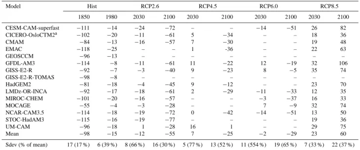
Table 1. Tropospheric ozone burdens (Tg) for the individual models and the ACCMIP mean. Also shows which simulations and time slices are available from each model for this study. Not all relevant variables are available for each model/time slice.

Model Hist RCP2.6 RCP4.5 RCP6.0 RCP8.5 1850 1980 2000 2030 2100 2030 2100 2030 2100 2030 2100 CESM-CAM-superfast 192 288 302 278 230 – – 289 252 328 384 CICERO-OsloCTM2a 206 287 308 296 247 312 274 – – 326 343 CMAM 239 310 323 307 266 330 293 – – 342 371 EMAC 259 352 378 – – 379 342 – – 399 441 GEOSCCM 250 333 346 – – – – – – – – GFDL-AM3 264 370 378 367 317 389 356 390 359 410 484 GISS-E2-Rb 252c 337 344 341 304e 352 321e 352 339e 379 417e GISS-E2-R-TOMAS 261 350 359 – – – – – – – – HadGEM2 227 289 307 303 262 316 295 – – 330 377 LMDz-OR-INCAb 247c 322 339d 321 278e 342 310e 329 306e 351 374e MIROC-CHEM 239 321 341 325 283 – – 338 304 356 374 MOCAGE 272 322 327 323 299 – – 333 358 400 NCAR-CAM3.5 221 318 336 317 263 336 294 322 285 349 386 STOC-HadAM3 234 332 348 329 272 – – – – 367 385 UM-CAM 226 304 322 323 293 338 322 – – 351 397 Mean 239 322 337 319 276 344 312 336 309 357 395 Sdev ( % of mean) 22 (9 %) 24 (8 %) 23 (7 %) 22 (7 %) 25 (9 %) 26 (8 %) 26 (8 %) 31 (9 %) 35 (11 %) 26 (7 %) 36 (9 %)

a_{Simulations are a single year.}

b_{These models submitted transient simulations. Their “time slice” means represent 10-yr averages about the given decade, except as noted.} c_{Mean of 1850–1859.}

d_{Mean of 1996–2000 (when the transient simulation stops).} e_{Mean of 2091–2100.}

mode; i.e. the models are driven by sea-surface temper-ature (SST) and sea-ice concentrations (SICs). GISS-E2-R uniquely was run as a fully coupled ocean-atmosphere climate model, although the closely related GISS-E2-R-TOMAS model was run with SSTs and SICs prescribed. CICERO-OsloCTM2 and MOCAGE are chemical transport models (CTMs), with MOCAGE using offline meteorologi-cal fields from an appropriate simulation of a climate model, and CICERO-OsloCTM2 using offline meteorological fields from a single year of a reanalysis dataset. Except for the CTMs, and LMDz-OR-INCA, STOC-HadAM3 and UM-CAM, the calculated ozone concentrations are used in the climate model radiation code, making most of the models chemistry-climate models (CCMs).

The model chemical schemes vary greatly in their com-plexity (e.g. as measured by the number of species and re-actions), particularly in the range of non-methane VOCs (NMVOCs) that they simulate. Complexity ranges from the simplified and parameterized schemes of CMAM (no NMVOCs) and CESM-CAM-superfast (isoprene as the only NMVOC), to the intermediate schemes of HadGEM2 and UM-CAM (include ≤ C3-alkanes), to the more complex

schemes of the other models, which include the more reac-tive, chiefly anthropogenic NMVOCs (e.g. higher alkanes, alkenes and aromatic species), as well as lumped monoter-penes. Some representation of stratospheric chemistry is in-cluded in many models, with the exception of CICERO-OsloCTM2, HadGEM2, LMDz-OR-INCA, STOC-HadAM3 and UM-CAM. CICERO-OsloCTM2 uses monthly-varying

climatological ozone values from a previous model sim-ulation (except for the lowest ∼2.5 km of the sphere), LMDz-OR-INCA uses a constant (in time) strato-spheric ozone climatology (Li and Shine, 1995), whereas the other models without detailed stratospheric chemistry used the time varying stratospheric ozone dataset of Cionni et al. (2011).

2.2 Scenarios and time slices

The ACCMIP simulations broadly correspond with the CMIP5 scenarios (Taylor et al., 2012). Historical (hereafter Hist) simulations cover the preindustrial period to the present day, while a range of Representative Concentration Pathways (RCPs) (van Vuuren et al., 2011) cover 21st century pro-jections. These latter scenarios are named for their nominal radiative forcing level (2100 compared to 1750), such that RCP2.6 corresponds to 2.6 Wm−2, RCP4.5 to 4.5 Wm−2, RCP6.0 to 6.0 Wm−2and RCP8.5 to 8.5 Wm−2. Ozone pre-cursor emissions from anthropogenic and biomass burning sources were taken from those compiled by Lamarque et al. (2010) for the Hist simulations, whereas emissions for the RCP simulations are described by Lamarque et al. (2013) (see also Lamarque et al., 2011; van Vuuren et al., 2011). Excluding methane emissions, all the RCPs include reduc-tions and redistribureduc-tions of ozone precursor emissions mov-ing through the 21st century. Natural emissions, such as CO and VOCs from vegetation and oceans, and NOxfrom soils

and lighting, were determined by each model group. The

emissions used by the individual models are discussed fur-ther in Sect. 3.

With the exception of GISS-E2-R and LMDz-OR-INCA, each model conducted a set of time slice simulations for each scenario. In this study, we analyse output from the 1850, 1980 and 2000 time slices from the Hist scenario, and the 2030 and 2100 time slices for the RCPs, to provide near-term and longer-near-term perspectives. Except for the CTMs and GISS-E2-R, each model used climatological SSTs and SICs from coupled ocean-atmosphere CMIP5 simulations of a closely related climate model, typically averaged for the 10 yr about each time slice (e.g. 2026–2035 for the 2030 time slice), although some models had interannually varying boundary conditions. CICERO-OsloCTM2 used the same meteorology for each simulation, whereas MOCAGE was run with meteorological fields from a climate model running the appropriate time slice and scenario, rather than directly using the SSTs and sea-ice to drive an atmosphere model. The number of years that the ACCMIP models simulated for each time slice mostly varied between 4 and 12 yr for each model, although CICERO-OsloCTM2 only simulated a single year. However, as the boundary conditions (including biomass burning emissions) were constant for each year of a given time slice for most models, “interannual” variability is generally small (see Sect. 4).

GISS-E2-R and LMDz-OR-INCA both conducted tran-sient simulations, and the data analysed in this study were averaged for the decade about each time slice (e.g. 1976– 1985 for the 1980 time slice), with some minor exceptions as noted in Table 1.

2.3 Analyses: tropopause definition and statistical definitions

Throughout this analysis, the troposphere is defined as air with ozone concentrations less than or equal to 150 ppbv (Prather et al., 2001), which is simple to employ and allows comparison against other model studies (e.g. Stevenson et al., 2006). For a consistent definition of the troposphere for all time slices, the definition is applied using the ozone from the Hist 1850 time slice mean, applied on a per model basis, and varying by month. We used the 1850 time slice to avoid issues with different degrees of stratospheric ozone depletion across the ensemble, particularly in the Southern Hemisphere (SH). While fixing the definition means we compare a consis-tent region of the atmosphere between different time slices, it does ignore the fact the tropopause height will likely alter with climate change (Santer et al., 2003a, b). Furthermore, values for the tropospheric ozone burdens and columns are obviously sensitive to the tropopause definition (Wild, 2007; Prather et al., 2011), and the differences generally amount to

±5 % compared to using the 2000 time slice mean ozone, al-though they can exceed 10 % for a few models for the RCPs. We apply a pressure based tropopause definition to ensure a

consistent comparison of the modelled tropospheric column ozone against satellite data in Sect. 4.2.

A statistical analysis of whether the projected ozone changes are significant against interannual variability is not possible with the ACCMIP data, mainly because the inter-annual variability is insufficiently characterised by the time slice runs, as most have constant SSTs and SICs on a year-to-year basis, and all have constant biomass burning emis-sions. Instead, we assess whether a given multi-model mean ozone change is significantly different from zero by using a paired sample Student’s t test (e.g. Wilks, 2006). Changes are considered significant if the (absolute) mean change from all the models is greater than 2 times the standard error for the mean change (i.e. approximately the 5 % level). One weak-ness of this analysis is that it cannot highlight regions where the models agree that the changes are not significant with re-spect to interannual variability (see Tebaldi et al., 2011).

For the most part, output from the models was interpo-lated to the grid used by Cionni et al. (2011), who compiled the ozone dataset recommended for use in the CMIP5 sim-ulations (5◦by 5◦latitude/longitude and 24 pressure levels). However, the tropospheric burden and columns were calcu-lated on a model’s native grid.

3 Emissions: differences and similarities between models

While one goal of ACCMIP was for models to match each other’s ozone precursor inputs as closely as possible, differ-ences in model parameterisations and complexity means that some model diversity is unavoidable. In particular, natural emissions were not prescribed as part of the experimental de-sign, and their differing treatment between models broadens the range of ozone precursors. Such differences are examples of why we need model comparisons.

Figure 1 shows the range in ozone precursor emissions in the ACCMIP models, presenting box-whisker plots for each scenario and time slice. The number of models that constitute the spread of the data is different for different simulations – see Table 1. Tabulated emission data for the individual mod-els can be found in Table S1 in the Supplement.

Figure 1a shows that the tropospheric methane burden is generally well constrained in the simulations, with the in-terquartile range (IQR) being 3–5.5 % of the mean burden. The close agreement is due to all models except LMDz-OR-INCA having used prescribed methane surface con-centrations for the Hist simulations, and only GISS-E2-R and LMDz-OR-INCA not prescribing concentrations for the RCP simulations. The methane burden approximately dou-bles from 1850 to 2000, but 2100 burdens are 30 %, 10 % and 2.5 % lower than 2000, for the RCP2.6, RCP4.5 and RCP6.0 scenarios respectively. For RCP8.5, by 2100 the methane burden has more than doubled again compared to 2000.

time slice 14 Historical 14 14 12 RCP2.6 12 8 RCP4.5 8 7 RCP6.0 7 13 RCP8.5 13 1850 1980 2000 2030 2100 2030 2100 2030 2100 2030 2100 time slice 400 600 800 1000 1200 1400 1600 1800 Tg CO a−1 13 Historical 13 13 11 RCP2.6 11 8 RCP4.5 8 7 RCP6.0 7 12 RCP8.5 12 1850 1980 2000 2030 2100 2030 2100 2030 2100 2030 2100 time slice 0 200 400 600 800 1000 1200 Tg C a−1 14 Historical 14 14 12 RCP2.6 12 9 RCP4.5 9 7 RCP6.0 7 13 RCP8.5 13 1850 1980 2000 2030 2100 2030 2100 2030 2100 2030 2100 time slice 0 20 40 60 Tg N a−1 12 Historical 12 12 10 RCP2.6 10 7 RCP4.5 7 7 RCP6.0 7 11 RCP8.5 11 1850 1980 2000 2030 2100 2030 2100 2030 2100 2030 2100 time slice 0 200 400 600 800 1000 1200 Tg C a−1 14 Historical 14 14 12 RCP2.6 12 9 RCP4.5 9 7 RCP6.0 7 12 RCP8.5 13 1850 1980 2000 2030 2100 2030 2100 2030 2100 2030 2100 time slice 0 5 10 15 Tg N a−1 12 Historical 12 12 10 RCP2.6 10 8 RCP4.5 8 6 RCP6.0 6 11 RCP8.5 11 1850 1980 2000 2030 2100 2030 2100 2030 2100 2030 2100 0 50 100 150 200 250 300 Tg C a−1 13 Historical 13 13 10 RCP2.6 11 8 RCP4.5 9 6 RCP6.0 6 11 RCP8.5 12 1850 1980 2000 2030 2100 2030 2100 2030 2100 2030 2100 time slice 2000 4000 6000 8000 10000 Tg

(a) Methane burden

(b) CO

(e) Total VOC

(c) Total NOx

(f) Biogenic VOC

(d) LNOx

(g) Other VOC

Fig. 1. Burdens and emissions of ozone precursors used in the ACCMIP scenarios and time slices, showing (a) the tropospheric methane burden, and yearly total (b) CO emissions, (c) total NOxemissions, (d) lightning NOxemissions and (e) total VOC emissions, which are

then split into (f) biogenic VOCs and (g) other VOCs. The spread of the emissions/burden in each model is indicated for each scenario and time slice, with filled box showing the interquartile range, the whiskers indicating the full range, and the dot and line indicating the mean and median respectively. Not all models completed all the scenarios: the number of models used to determine each box/whisker is indicated.

The general trends in CO (Fig. 1b) and total NOx(Fig. 1c)

emissions are similar, increasing from 1850 to 2000 for the Hist scenario, decreasing thereafter for all the RCPs, ex-cept for the 5 % higher NOx emissions for the 2030 time

slice of RCP8.5, compared to Hist 2000. NOx emissions

show a stronger increase over the 20th century, with the mean trebling between 1850 and 2000, whereas CO

emis-sions slightly more than double. Across all RCPs, by 2100 CO and NOxemissions are lower by 30–45 % compared to

2000.

Both CO and NOxemissions show a greater degree of

vari-ation between the models than the methane burden. For a given time slice, the IQRs vary between approximately 10– 30 % of the corresponding mean emission, whereas the full

range (maximum minus minimum emission) is between 20– 100 % of the mean emission. The spread is due to the vary-ing natural emissions (NOx from soils and lightning; CO

from oceans and vegetation), as well as the less complex chemistry schemes used in some models including extra CO emissions as a surrogate for missing NMVOCs (e.g. CMAM, HadGEM2).

An example of the variation in natural emissions can be seen from Fig. 1d, which shows the spread in the lightning NOx source (LNOx) for the models. Parameterisations for

LNOxare generally dependent on cloud top heights and

con-vective mass fluxes (e.g. Price and Rind, 1992; Allen and Pickering, 2002), which likely show large variability be-tween models, accounting for spread. The IQRs are gen-erally 40–55 % of the mean emission, and the full range is 90–170 % of the mean. The maximum emissions come from the MIROC-CHEM, whose LNOxwas set mistakenly

high (by 60 %) in the ACCMIP simulations. The minimum emissions (< 2 Tg N yr−1) are generally from the HadGEM2 LNOx (who also mistakenly implemented LNOx), although

emissions are also low for CMAM for the RCP simula-tions. Our knowledge of LNOx is generally poor, but

(ex-cluding HadGEM2 and MIROC-CHEM) LNOxfor the Hist

2000 simulation ranges between 3.8–7.7 Tg N yr−1, within the range of 5 ± 3 Tg N yr−1 estimated by Schumann and Huntrieser (2007) for a range of LNOxparameterisations.

Possible changes in lightning activity with climate change (e.g. Williams, 2009 and refs. therein) have been recognised as potentially important for LNOx and the subsequent

im-pact on tropospheric composition (e.g. Price and Rind, 1994; Hauglustaine et al., 2005; Fiore et al., 2006; Schumann and Huntrieser, 2007; Zeng et al., 2008), even if only the spatial distribution changes (Stevenson et al., 2005). An increase in LNOx from 2000 to 2100 (RCP8.5; strongest warming) is

generally robust across the ACCMIP models, and ranges in magnitude from 10–75 %. CMAM is an outlier in this case, with 45 % lower emissions for RCP8.5 2100 compared to Hist 2000. CMAM is also the only model using an LNOx

parameterisation based on the study of Allen and Picker-ing (2002). Jacobson and Streets (2009) also modelled lower LNOx in a warmer climate, using a different

parameterisa-tion based on cloud ice. Clearly further study is required into the implications of the use of different parameterisations for LNOx, and the different sensitivities across models.

Figure 1e shows the total VOC emissions used in the AC-CMIP models. As with LNOx, the emissions cover a wide

range and there is no clear trend in the mean across the simulations. Many of the reasons for the differences are fa-miliar from the above discussion, particularly the fact that some models include more VOC species than others. An-other reason for the spread in VOC emissions comes from treatment of VOCs of biogenic origin, particularly isoprene, which likely dominates the total NMVOC emissions (e.g. Guenther et al., 1995). Figure 1f shows the spread of bio-genic VOC emissions between the ACCMIP models; these

emissions are mostly isoprene. EMAC, GEOSCCM, GISS-E2-R and STOC-HadAM3 simulations were the only ones to include climate-sensitive isoprene emissions, and these are the only models with a positive change in VOC emissions between Hist 2000 and RCP8.5 2100, arising from the posi-tive temperature dependence of isoprene emission algorithms (e.g. Guenther et al., 2006; Arneth et al., 2007b). Arneth et al. (2011) noted that the isoprene emission computed from a given algorithm is sensitive to the input meteorological data and vegetation boundary conditions, giving further cause for variation in VOC emissions between models. For the rest of the ACCMIP ensemble, if they included isoprene chem-istry, constant present day isoprene emissions were used for all simulations. Figure 1g shows that the trend in the non-biogenic VOC emissions (anthropogenic plus biomass burn-ing) broadly resembles that of CO and NOx, albeit with the

range of VOC complexity resulting in a larger spread of the emission total between the models (IQR is 30–100 % of the mean emission).

4 Present day ozone distribution and model-observation comparison

This section presents the tropospheric ozone burden, the tro-pospheric ozone budget (for a limited subset of models), and the distribution of tropospheric ozone (surface, column and zonal mean) as simulated by the ACCMIP models for the Hist 2000 simulation. The ozone concentrations and columns from this simulation are then compared against observational datasets, from both satellites and ozonesondes. We do not over-interpret these comparisons since they exclude observa-tional error, and they differ in the periods covered. The em-phasis is largely on the distribution and measurement-model comparison for the ensemble mean, describing the spread of model results with statistical metrics. The distributions of ozone for all the individual models can be found in the sup-plementary material (Figs. S1–S3).

4.1 Tropospheric ozone burden and budget

Figure 2a shows the annual mean tropospheric ozone bur-den for all the models for Hist 2000, as well as the AC-CMIP mean. Values for the tropospheric burden for all mod-els and scenarios can also be found in Table 1. The mean burden is 337 ± 23 Tg, very close to the 336 ± 27 Tg re-ported for a subset of the ACCENT models (Stevenson et al., 2006) (344 ± 39 Tg for the full ACCENT ensemble), and the 335 ± 10 Tg estimated from measurement climatologies by Wild (2007), although the latter estimate is from pre-2000 ozone data. Figure 2a also indicates the uncertainty in the ozone burden, as represented by the standard deviation of the range of burdens computed for individual years of the time slice. As might be expected from successive years of the same boundary conditions (for most models), the uncertainty

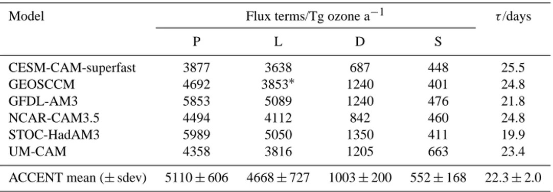
Table 2. Tropospheric ozone budget statistics for a subset of ACCMIP models for the Hist 2000 time slice, showing chemical production (P), chemical loss (L), deposition (D), the inferred stratospheric influx (S), and the lifetime (τ ).

Model Flux terms/Tg ozone a−1 τ/days

P L D S CESM-CAM-superfast 3877 3638 687 448 25.5 GEOSCCM 4692 3853∗ 1240 401 24.8 GFDL-AM3 5853 5089 1240 476 21.8 NCAR-CAM3.5 4494 4112 842 460 24.8 STOC-HadAM3 5989 5050 1350 411 19.9 UM-CAM 4358 3816 1205 663 23.4

ACCENT mean (± sdev) 5110 ± 606 4668 ± 727 1003 ± 200 552 ± 168 22.3 ± 2.0

∗_{Loss flux includes wet deposition of oxidised nitrogen compounds.}

49 1

Fig. 2. (a) Tropospheric ozone burdens for the ACCMIP models from the Hist 2000

2

simulations. Error bars for the models indicate the variability in the burden between different 3

years of a model’s time slice (± 1 std. dev.). The error bar on the ensemble mean burden 4

indicates the inter-model spread of the burden (± 1 std. dev.). (b) Distribution of the mean 5

ozone burden throughout the troposphere for the mean model, using the “boxes” 6

recommended by Lawrence et al. (2001) for reporting OH concentrations. The solid line 7

indicates the tropopause (see text for definition). 8 300 320 340 360 380 Tg CESM −CAM −superfast CICERO

−OsloCTM2CMAMEMAC_GEOSCCMGFDL

−AM3 GISS

−E2−R GISS

−E2−TOMASHadGEM2_{LMDzORINCAMIROC} −CHEM MOCAGE NCAR −CAM3.5 STOC −HadAM3UM−CAM ACCMIP mean 90S 30S EQ 30N 90N latitude 1000 700 500 250 pressure / hPa 4.6% 5.2% 6.7% 8.3% 4.3% 4.9% 5.7% 7.5% 10.4% 6.8% 7.6% 15.2% 6.4% 6.5% (b) 337 Tg ±0.6 % ±0.6 % ±0.8 % ±1.1 % ±0.5 % ±0.6 % ±0.4 % ±0.9 % ±1.2 % ±0.7 % ±0.6 % ±1.0 % ±0.8 % ±0.8 % (a)

Fig. 2. (a) Tropospheric ozone burdens for the ACCMIP models from the Hist 2000 simulations. Error bars for the models indicate the variability in the burden between different years of a model’s time slice (± 1 std. dev.). The error bar on the ensemble mean bur-den indicates the inter-model spread of the burbur-den (± 1 std. dev.). (b) Distribution of the mean ozone burden throughout the tropo-sphere for the mean model, using the “boxes” recommended by Lawrence et al. (2001) for reporting OH concentrations. The solid line indicates the tropopause (see text for definition).

is small, and the standard deviations are less than 2 % of the burden.

There is a significant correlation (r = 0.67) between the modelled ozone burden and the total VOC emissions. With the spread of VOC emission and treatment between the mod-els, it is difficult to rationalise this correlation satisfactorily, although Wild (2007) demonstrated increased VOC emis-sions lead to an increased ozone burden. There is not a simi-lar correlation between the ozone burden and total NOx

emis-sions.

Figure 2b indicates the distribution of the mean ozone bur-den throughout the troposphere, using the regions defined by Lawrence et al. (2001) (to describe the distribution of OH) to give a mass-weighted view of the zonal ozone distribu-tion. The hemispheric asymmetry in ozone is apparent from Fig. 2b, which shows that 57.5 % of the ozone mass is in the NH. The NH extratropics has 60 % more ozone than the SH extratropics overall, but the NH tropics has only slightly more ozone (∼3 %) than the SH tropics overall. The greatest burdens are found in the extratropical upper troposphere, re-flecting the importance of stratosphere-to-troposphere trans-port of ozone. The next largest ozone burdens are found in the comparatively more polluted NH lower troposphere, as well as the tropical upper troposphere. This latter region is im-pacted by convective transport of ozone precursors and light-ning emissions (Jacob et al., 1996). The standard deviation in the fractional distribution of ozone is also in Fig. 2b, show-ing that the model uncertainty in distribution of ozone mass is largest in the NH extratropics and in the upper troposphere in general, consistent with the results described in Sect. 4.2.

Table 2 presents the present day tropospheric ozone bud-get terms for the six models for which there are sufficient data. We do not report the ensemble mean result due to both the limited number of models and that the chemical produc-tion (P) and loss (L) terms were not calculated in a consis-tent manner (e.g. whether ozone loss through oxidised ni-trogen species was considered); ozone dry deposition (D) was calculated consistently for these models however. Fol-lowing Stevenson et al. (2006), the net influx of ozone from

50

2

3

Fig. 3. ACCMIP ensemble mean, annual mean ozone climatologies and their inter-model

4

variability, for the 2000 time slice of the Historical simulation. Top row shows zonal mean

5

ozone, the middle row shows the tropospheric ozone column, and the bottom row shows

6

surface ozone. For each row, the left hand panels show the absolute values of the ozone

7

variable: ppbv for the zonal mean and surface concentrations, and Dobson units (DU) for the

8

tropospheric column. The middle panels show the absolute standard deviations in the same

9

units. The right hand column expresses the standard deviation as a percentage of the ensemble

10

mean value (also known as the coefficient of variation). Note that each panel has a different

11

scale.

12

13

(a) Zonal mean conc (ppbv) (b) Zonal mean sdev (ppbv) (c) Zonal mean sdev (%)

(d) Trop column (DU) (e) Trop column sdev (DU) (f) Trop column sdev (%)

(g) Surface conc (ppbv) (h) Surface sdev (ppbv) (i) Surface sdev (%)

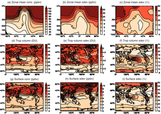
Fig. 3. ACCMIP ensemble mean, annual mean ozone climatologies and their inter-model variability, for the 2000 time slice of the Historical simulation. Top row shows zonal mean ozone, the middle row shows the tropospheric ozone column, and the bottom row shows surface ozone. For each row, the left hand panels show the absolute values of the ozone variable: ppbv for the zonal mean and surface concentrations, and Dobson units (DU) for the tropospheric column. The middle panels show the absolute standard deviations in the same units. The right hand column expresses the standard deviation as a percentage of the ensemble mean value (also known as the coefficient of variation). Note that each panel has a different scale.

the stratosphere (Sinf) is calculated from the residual of the

other terms (Sinf= P – L + D), and the tropospheric ozone

lifetime (τ ) is calculated using the burdens (B) in Table 1 (τ = B/F, where F = L + D = P + Sinf). As with the burden, all

flux terms are defined using the 150 ppbv ozone contour as the tropopause (from Hist 1850).

Several differences are apparent from comparing the AC-CMIP results against the ACCENT study (the ACCENT mean data are shown in Table 2), although we caution that, with the limited amount of ACCMIP data, generalisations about how the modelled budget has changed since ACCENT are hard to make. For GFDL-AM3 and STOC-HadAM3, P is much higher than the ACCENT mean, whereas P is much lower for CESM-CAM-superfast, NCAR-CAM3.5 and UM-CAM. For L, the ACCMIP models are broadly ordered the same as P, although – unlike P – all the L terms all sit within the range described by the ACCENT mean and stan-dard deviation. The ACCMIP models with the lower P and L have lower total VOC emissions (see Table S1b), which could go some way to explaining the range in Table 2 (e.g. Wild, 2007). These models also have the longest tropospheric ozone lifetimes. For D, the ACCMIP results span nearly a

factor of two between CESM-CAM-superfast and STOC-HadAM3. The fact that D does not simply correlate with B underlines that there are differences in the ozone spatial distribution and the deposition implementation between the models (see Lamarque et al., 2013), which has implications for assessing the impacts of ozone concentration changes on the biosphere (e.g. Sitch et al., 2007). For Sinf, all the

AC-CMIP models are encompassed by the ACCENT mean and standard deviation, and, furthermore, Sinffor the six models

is within the 540 ± 140 Tg yr−1range suggested using obser-vational constraints of stratosphere-to-troposhere exchange (Olsen et al., 2001; Wild, 2007). However, determining the net stratospheric influx by budget closure will likely give a different value to that calculated using transport diagnostics within the model (e.g. Sanderson et al., 2007), and – as with all the budget terms – there will be some sensitivity to the tropopause definition (Wild, 2007).

4.2 Zonal mean, tropospheric column and surface ozone from Hist 2000

Figure 3 shows the ensemble mean, annual mean distribu-tion of ozone, presenting the zonal mean, tropospheric col-umn and surface ozone concentrations, as well as their inter-model variability. The general patterns of the ozone distribu-tion in Figs. 3a, 3d and 3g are consistent with those reported from satellite (Fishman et al., 1990; Ziemke et al., 2011) and ozonesonde (Logan, 1999; Thompson et al., 2003) measure-ments, as well as the multi-model data shown by Stevenson et al. (2006). The increase in ozone concentration with height is clear, in accordance with the increase in ozone lifetime. Con-vective lifting of low-ozone air masses coupled with lofting of ozone precursors (Lawrence et al., 2003; Doherty et al., 2005) results in the characteristic tropical zonal mean profile in Fig. 3a. The hemispheric asymmetry in mid-tropospheric ozone concentrations reflects the larger input of stratospheric ozone in the NH, due to the stronger Brewer-Dobson circula-tion there (Rosenlof, 1995), as well as the larger emissions of ozone precursors (Lamarque et al., 2010). While both the tropospheric column (Fig. 3d) and surface concentrations (Fig. 3g) also show higher ozone levels over ozone precur-sor source regions, the plots also indicate enhanced concen-trations downwind of the these regions, due to transport of ozone and ozone precursors, including “reservoir” species, such as PAN (Moxim et al., 1996; Fiore et al., 2009). Fig-ure 3d also shows the “wave-1” pattern in the tropical tro-pospheric ozone column (Thompson et al., 2003; Ziemke et al., 2011), with a minimum in ozone over the Pacific Ocean and maximum over the Atlantic. Surface ozone concentra-tions are also very low over the equatorial Pacific Ocean.

There is generally good agreement between the models for the zonal mean profile of ozone. Figure 3c shows that the standard deviation is less than 20 % of the mean throughout much of the troposphere, with exception of some lower tro-posphere regions and the upper trotro-posphere. The spatial pat-terns of the spread in surface ozone concentrations in Fig. 3h and i suggest that much of the lower troposphere variability is over regions with large anthropogenic, pyrogenic or biogenic emissions, where both the absolute and relative uncertainty is largest. In anthropogenic and biomass burning source re-gions, much of the model diversity could reflect the spread in VOC composition (low vs. high reactivity species), which means different ozone production efficiencies (e.g. Russell et al., 1995), as well as using different injection heights for biomass burning emissions. For tropical Africa and espe-cially South America, large variations are apparent over iso-prene source regions (surface and column), which reflects differences in the total emission (some models have no iso-prene), as well as potentially differences in isoprene chem-istry (Archibald et al., 2010).

Large model variation is also found for the high latitude SH, chiefly for the tropospheric column. Tropospheric ozone levels in the SH are generally low, but there is relatively

large diversity in the overhead stratospheric ozone column (standard deviation for the total ozone column is 10–15 % of the mean; not shown). This results in a spread in the strato-spheric input as well as potentially some impacts through changes in photolysis rates, for those models with photolysis schemes that use the model-calculated ozone column (e.g. Fuglestvedt et al., 1994; see also Voulgarakis et al., 2012). There is less (relative) variation in the tropospheric column in the Northern Hemisphere (NH), coupled with less spread between models for the total ozone column (not shown). But larger uncertainty for the surface at high latitudes could be re-lated to differences in precursor transport and chemistry from lower latitudes (Eckhardt et al., 2003; Shindell et al., 2008; Christoudias et al., 2012). As was also found by Stevenson et al. (2006), there are large relative uncertainties in tropo-spheric column ozone over the equatorial Pacific Ocean, but the concentrations here are very low.

4.3 Comparison to ozonesondes and satellite data

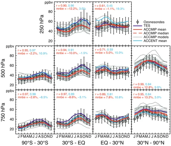
Figure 4 compares the ACCMIP mean, median and indi-vidually modelled ozone concentrations from the Hist 2000 simulation against ozonesonde data, in the same manner as Stevenson et al. (2006). Ozonesonde measurements are taken from datasets described by Logan (1999) (representa-tive of 1980–1993) and Thompson et al. (2003) (represen-tative of 1997–2011), and consist of 48 stations, split 5, 15, 10 and 18 between the SH extratropics, SH tropics, NH trop-ics and NH extratroptrop-ics respectively. The models were sam-pled at the ozonesonde locations. In addition, Fig. 4 shows satellite-derived ozone concentrations retrieved from the Tro-pospheric Emission Spectrometer (TES), which is a Fourier transform spectrometer on board the NASA Aura spacecraft in 2004 (Beer, 2006). TES ozone from a 2005–2010 climatol-ogy was interpolated to the same grid as the ACCMIP mod-els and sampled at the ozonesonde locations. Figure 4 also shows the ACCENT model mean (Stevenson et al., 2006), to place the ACCMIP results in context of recent multi-model comparisons. The correlation and mean normalised bias er-ror (MNBE) are shown for multi-model mean from the AC-CMIP and ACCENT ensembles, relative to the ozonesonde observations.

Both the ACCMIP ensemble mean and median are within the standard deviation of the observations for most loca-tions and altitudes, with the winter NH extratropical com-parison being a notable exception. Indeed, compared to the mean observations, the largest relative errors are found for the NH extratropics, where the mean model overesti-mates the concentrations, and SH tropics, where the mean model underestimates the concentrations. The individual model biases in these locations are significantly correlated with total VOC emissions (r = 0.57; i.e. more VOC emis-sions give a more positive, or less negative, bias), although several other chemical and transport factors likely play a role. However, the mean model captures the annual cycle

J F M A M J J A S O N D 20 40 60 80 J F M A M J J A S O N D 20 40 60 80 100 J F M A M J J A S O N D 20 40 60 80 J F M A M J J A S O N D 20 40 60 80 100 J F M A M J J A S O N D 20 40 60 80 100 J F M A M J J A S O N D 20 40 60 80 100 J FMAM J J A SOND 20 40 60 80 J FMAM J J A SOND 20 40 60 80 100 J FMAM J J A SOND 20 40 60 80 100 J FMAM J J A SOND 20 40 60 80 100 ppbv TES ACCMIP mean ACCMIP median ACCMIP models ACCENT mean r = 0.90, 0.96 mnbe = −12.2%, 3.0% r = 0.61, mnbe = −1.1%, 0.45 19.3% r = 0.95, 0.97 mnbe = −2.2%, 10.9% r = 0.94, 0.91 mnbe = −10.0%, −1.5% r = 0.71, 0.59 mnbe = 5.0%, 15.0% r = 0.99, 0.84 mnbe = 12.8%, 9.9% r = 0.97, 0.98 mnbe = −2.6%, −8.5% r = 0.97, 0.89 mnbe = −8.6%, −3.1% r = 0.89, mnbe = 7.8%, 0.81 10.8% r = 0.95, 0.84 mnbe = 13.2%, 3.0% ppbv ppbv

2

5

0

h

Pa

5

0

0

h

Pa

7

5

0

h

Pa

90°S - 30°S

30°S - EQ

EQ - 30°N

30°N - 90°N

Fig. 4. Comparison of the annual cycle of ozone, between ozonesonde observations (black circles) and the ACCMIP ensemble mean (solid red line), ACCMIP ensemble median (dashed red line) and the ACCENT ensemble mean (blue line) (Stevenson et al., 2006). Ozone concen-trations from TES (purple line) are also shown. ACCMIP model data is from the 2000 time slice mean of the Historical experiment. Model and observational data were grouped into four latitude bands (90◦S to 30◦S, 30◦S to 0◦, 0◦to 30◦N and 30◦N to 90◦N) and sampled at three altitudes (700 hPa, 500 hPa and 250 hPa), with the models sampled at the ozonesonde locations before averaging together. The individ-ual ACCMIP models are represented by the thin grey lines, with the grey shaded area indicating ± 1 standard deviation about the ACCMIP ensemble mean, showing the model spread. Error bars on the observations indicate the average interannual standard deviation for each group of stations. The correlation (r) and mean normalised bias error (mnbe) for the ACCMIP (red) and ACCENT (blue) ensemble means versus the observations are also indicated in each panel. This figure is an update of Fig. 2 of Stevenson et al. (2006).

in ozone concentrations extremely well in most locations (as measured by the correlation coefficient), suggesting that, broadly speaking, the seasonality in circulation patterns, stratosphere-to-troposphere exchange and natural emissions (chiefly biomass burning in the tropics, and isoprene in the NH extratropics) is captured well. The statistics for the NH tropical mid and upper troposphere suggest that the season-ality is less well modelled, although we note that, (1) the observed-model correlation is significant (r > 0.58), (2) there is considerable observed interannual variability in ozone the upper troposphere, and (3) the bias and correlation are im-proved compared to the ACCENT mean. Compared to AC-CENT, the correlation is improved with the ACCMIP mean model for most locations, and the bias for some locations, both most prominently in the NH.

Except for the NH Tropics at 250 hPa, the TES data are positively biased compared to the ozonesondes, broadly

con-sistent with the 2–10 ppbv high bias that Nasser et al. (2008) noted for TES (see also Zhang et al., 2010). However, taking the interannual variability into account, and the fact that we have neither applied the TES operators in this analysis (Wor-den et al., 2007), nor considered measurement uncertainty, the TES and ozonesonde data are not notably different. This positive bias means that, compared to the ozonesonde data, the ACCMIP mean model bias against TES is improved for the NH extratropics, about the same for the NH tropics (op-posite in sign), but worsened for the SH; changes in cor-relation compared to the ACCMIP-ozonesonde comparison are marginal. As mentioned above both the ozonesondes and TES see a sharp increase in ozone between March and April at EQ–30◦N, not captured in the ACCMIP mean. TES (and several ACCMIP models) do not show the same low values in the winter months as the ozonesonde data. For TES, this is likely due to lower thermal contrast which will make the

250 hPa

SH polar SH midlat Atlantic/Africa Equatorial Americas W Pacific/E Indian Ocean NH sub−tropics Japan West Europe Eastern US Canada NH Polar east NH Polar west −60 −40 −20 0 20 40 60 MN BE (% )

500 hPa

SH polar SH midlat Atlantic/Africa Equatorial Americas W Pacific/E Indian Ocean NH sub−tropics Japan West Europe Eastern US Canada NH Polar east NH Polar west −60 −40 −20 0 20 40 60 MN BE (% )

700 hPa

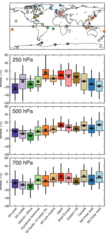
Fig. 5. Normalised biases for the ACCMIP models (Hist 2000 simu-lation) against the ozonesonde measurements compiled into regions by Tilmes et al. (2012). Each region is colour-coded, and the con-stituent ozonesonde sites are indicated in the top panel. Biases are shown for (bottom to top) 750, 500 and 250 hPa. The box, whiskers, line and dot show the interquartile range, full range, median and mean biases respectively, in a similar style to Fig. 1. The y-axis has the same scale in each panel.

satellite retrievals relax to an a priori value (Bowman et al., 2006). Bowman et al. (2012) pursue comparisons of the AC-CMIP models against TES further.

Figure 5 makes a similar comparison to ozonesonde data, this time using the compilation of Tilmes et al. (2012). This dataset mostly consists of the same station data described by Logan (1999) and Thompson et al. (2003), but covering 1995–2009, and aggregated into 12 regions that exhibit sim-ilar ozone concentration characteristics (see the top panel of Fig. 5 and Tilmes et al., 2012). The figure presents the mean, median and spread of the MNBE for the individual ACCMIP models (cf. Fig. 1), showing that the full range of perfor-mance encompasses positive and negative biases for each re-gion and altitude.

The information in Fig. 5 is consistent with that in Fig. 4, but with more longitudinal information. For instance, we see that the negative bias in the SH tropical ozone is driven by the less favourable comparison of the model mean with the sites in the Atlantic/Africa region (dark green), and the sign of the bias is consistent across more than 75 % of the models. A positive bias is apparent in all the NH extratrop-ical regions in the low and mid-troposphere, and again is shared by the majority of the models. Figure 5 also shows low biases for the high latitude regions in the upper tro-posphere/lower stratosphere (UT/LS; a region not shown in Fig. 4). A comparison of the ACCMIP mean total ozone col-umn against satellite measurements from the merged Total Ozone Mapping Spectrometer/solar backscatter ultraviolet (TOMS/SBUV) data (Stolarski and Frith, 2006) suggests that the models overestimate the total ozone column by around 5 % at high latitudes (not shown), although the total column bias is not necessarily related to UT/LS biases. Validation of stratospheric ozone in these models is beyond the scope of this study, but this would help resolve whether ozonesonde-model comparisons at higher altitudes are consistent with the satellite data. (A comparison of the ensemble mean ozone column against TOMS data can be found in the supplemen-tary material, along with a comparison of late twentieth cen-tury trends.)

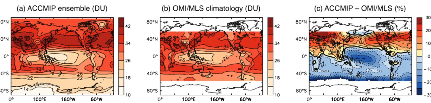
Tropospheric ozone columns are available from a combi-nation of the Ozone Monitoring Instrument (OMI) and Mi-crowave Limb Sounder (MLS) data. Figure 6 compares the ACCMIP mean tropospheric column ozone against the OMI-MLS climatology derived by Ziemke et al. (2011), covering October 2004 to December 2010. Tables 3 and 4 summarise the comparisons between the OMI/MLS data and individual models, showing the global (60◦_S–60◦_{N) column biases and} spatial correlations, and biases by latitude bands respectively. For each model, the column was defined using the tropopause pressures provided by Ziemke et al. (2011) (from the Na-tional Centers for Environmental Prediction, NCEP), mean-ing that Fig. 6a is subtly different from Fig. 2d.

From Table 3, the global, ensemble mean tropospheric ozone column is 30.8 DU, compared to 31.1 DU for OMI/MLS, although the latter has a root-mean square

(a) ACCMIP ensemble (DU) (b) OMI/MLS climatology (DU) (c) ACCMIP – OMI/MLS (%)

Fig. 6. Comparison of the annual mean tropospheric ozone column between (a) the ACCMIP ensemble (different tropopause compared to Fig. 2d) and (b) a climatology derived from the Ozone Monitoring Instrument (OMI) and Microwave Limb Sounder (MLS) by Ziemke et al. (2011). (c) ACCMIP ensemble bias compared to OMI/MLS (%). See also Tables 2 and 3.

Table 3. Tropospheric ozone column, bias and spatial correation for the Hist 2000 simulation of the ACCMIP models vs. a climatology derived from OMI data (Ziemke et al., 2011).

Models Column/DU Bia/DU r

CESM-CAM-superfast 26.2 −4.9 0.79 CICERO-OsloCTM2 28.3 −2.8 0.84 CMAM 30.3 −0.8 0.87 EMAC 34.8 3.7 0.84 GEOSCCM 32.1 1.1 0.87 GFDL-AM3 35.1 4.0 0.89 GISS-E2-R 33.7 2.6 0.85 GISS-E2-R-TOMAS 34.7 3.6 0.87 HadGEM2 28.6 −2.4 0.83 LMDz-OR-INCA 31.2 0.1 0.87 MIROC-CHEM 31.3 0.2 0.81 MOCAGE 28.8 −2.2 0.60 NCAR-CAM3.5 28.9 −2.2 0.84 STOC-HadAM3 28.7 −2.4 0.81 UM-CAM 29.7 −1.4 0.75

ACCMIP mean (± sdev) 30.8 −0.4 ± 2.7 0.87 ± 0.07

interannual variability of ∼3 DU (Ziemke et al., 2011), which overlaps an additional observationally-based estimate from the TES instrument of 29.8–32.8 DU (H. Worden, personal commnication, 2012). The range from these two instruments encompasses the columns calculated by 75 % of the models. The spatial correlation between OMI/MLS and the models is generally very high (cf. Fig. 6a and b).

Many of the differences between the ensemble mean and OMI/MLS are broadly consistent with the comparison against ozonesonde data (Fig. 6c; Table 4), and biases in the mean column for a given latitude band are well correlated with those for the ozonesondes (r ≥ 0.75 for any pressure level). Compared to OMI/MLS, the ensemble mean overes-timates the column across the NH mid-latitudes, and under-estimates the column over tropical oceans and for all regions poleward of approximately 30◦S, although the underestimate is stronger than suggested by the ozonesonde data. The nega-tive bias over the equatorial Pacific in Fig. 6c is not consistent with the ozonesonde comparison in Fig. 5, which suggests a

neutral or positive bias for the mean model. However, this region is poorly represented by ozonesonde measurements. Correlations between the biases for the NH and SH tropical columns are strong (r = 0.88), suggesting that similar pro-cesses are operating in the regions, even if the sign of the bias is different between them (i.e. a model with a stronger positive NH tropical bias likely has a SH tropical bias that is either positive, or less negative than the ensemble mean).

Overall, compared to the ensemble of observations, the models may have a systematic high bias in the NH, and a sys-tematic low bias in the SH. As the emissions are broadly con-sistent across the ensemble, the prevalence of this bias could suggest they are deficient in some way, in either their amount or distribution, or both. However, the models all typically fall within the interannual variability of the observations.

5 Tropospheric ozone from 1850 to 2100

In this section we consider the changes in tropospheric ozone projected by the ACCMIP models for the past (1850 and 1980), as well as for the near (2030) and more distant (2100) future, using the range of RCPs. We begin by discussing global-scale changes, followed by regional changes, before considering the drivers of the change.

5.1 Global-scale changes: tropospheric ozone burden

Figure 7a shows the annual average tropospheric ozone bur-den for the ACCMIP models for all the simulations and time slices considered. Figure 7b shows the difference in the tro-pospheric ozone burden compared to the Hist 2000 simula-tion. Data for individual models burdens and their differences can be found in Tables 1 and 5 respectively.

The evolution of the mean tropospheric burden in Fig. 7a shows a 25 % increase between 1850 and 1980, and a 29 % increase between 1850 and 2000 (very close to the results of Lamarque et al., 2005); the burden increases by 4 % be-tween 1980 and 2000. Future projections vary with the sce-nario. Compared to the mean 2000 burden of 337 Tg, the rel-ative changes in the mean burdens for 2030 (2100) for the

Table 4. Tropospheric ozone column and bias (DU) for the Hist 2000 simulation of the ACCMIP models vs. the OMI climatology for different latitude bands.

60◦S–30◦S 30◦S–Eq. Eq.–30◦N 30◦N – 60◦N Col Bias Col Bias Col Bias Col Bias CESM-CAM-superfast 21.9 −7.8 21.6 −8.4 26.0 −5.0 37.2 3.1 CICERO-OsloCTM2 22.1 −7.6 27.5 −2.5 30.0 −1.0 33.2 −0.9 CMAM 29.1 −0.6 27.5 −2.4 29.3 −1.7 36.5 2.4 EMAC 29.4 −0.3 33.9 3.9 36.7 5.7 38.6 4.5 GEOSCCM 28.4 −1.3 28.8 −1.2 32.0 1.0 40.6 6.5 GFDL-AM3 31.4 1.7 31.8 1.9 35.2 4.2 42.9 8.8 GISS-E2-R 27.4 −2.3 29.0 −1.0 33.5 2.5 46.5 12.4 GISS-E2-R-TOMAS 30.0 0.2 30.5 0.5 33.8 2.8 46.3 12.2 HadGEM2 22.8 −6.9 26.4 −3.6 31.1 0.1 34.2 0.1 LMDz-OR-INCA 25.7 −4.0 29.2 −0.8 31.9 0.9 38.3 4.2 MIROC-CHEM 25.1 −4.6 31.4 1.4 33.8 2.7 34.1 −0.0 MOCAGE 18.9 −10.8 24.5 −5.5 32.3 1.3 40.0 5.9 NCAR-CAM3.5 25.1 −4.7 24.7 −5.3 29.4 −1.6 37.6 3.6 STOC-HadAM3 21.5 −8.3 26.1 −3.8 31.2 0.2 35.8 1.7 UM-CAM 26.2 −3.5 23.8 −6.1 30.4 −0.6 40.4 6.3 ACCMIP mean (± sdev) 25.7 ± 3.7 -4.1 27.8 ± 3.4 -2.2 31.8 ± 2.7 0.8 38.8 ± 4.1 4.7

OMI (obs) 29.7 30.0 31.0 34.1

Table 5. Differences in the tropospheric ozone burden compared to Hist 2000, using data in Table 1.

Model Hist RCP2.6 RCP4.5 RCP6.0 RCP8.5 1850 1980 2030 2100 2030 2100 2030 2100 2030 2100 CESM-CAM-superfast −111 −14 −24 −72 – – −14 −51 26 82 CICERO-OsloCTM2a −102 −20 −11 −61 5 −34 – – 18 36 CMAM −84 −13 −16 −57 7 −30 – – 19 48 EMAC −118 −25 – – 1 -36 – – 22 63 GEOSCCM −96 −13 – – – – – – – – GFDL-AM3 −114 −8 −11 −61 11 −22 12 −19 32 106 GISS-E2-R −92 −7 −3 −40 9 −23 8 −5 35 74 GISS-E2-R-TOMAS −98 −8 – – – – – – – – HadGEM2 −81 −18 −4 −45 9 −12 – – 23 70 LMDz-OR-INCA −92 −17 −18 −61 2 −29 −11 −33 12 35 MIROC-CHEM −101 −20 −16 −57 – – −3 −37 16 33 MOCAGE −55 −4 −3 −28 – – 7 −9 32 74 NCAR-CAM3.5 −114 −18 −19 −72 0 −42 −14 −51 13 50 STOC-HadAM3 −115 −16 −19 −77 – – – – 19 36 UM-CAM −96 −18 1 −28 16 1 – – 29 75 Mean −98 −15 −12 −55 7 −25 −2 −29 23 60 Sdev (% of mean) 17 (17 %) 6 (39 %) 8 (66 %) 16 (30 %) 5 (77 %) 13 (52 %) 11 (554 %) 19 (65 %) 7 (33 %) 22 (37 %)

different RCPs are: −4 % (−16 %) for RCP2.6, 2 % (−7 %) for RCP4.5, −1 % (−9 %) for RCP6.0, and 7 % (18 %) for RCP8.5. RCP8.5 is the only scenario to show an ozone increase for both time slices (23 Tg and 60 Tg), whereas RCP4.5 shows an increase in 2030 (7 Tg), before decreas-ing in 2100 (−25 Tg). The ozone burden for the 2030 time slice of RCP6.0 is unchanged compared to 2000, although it is still higher than 1980.

Figure 7 also shows a large range in the modelled ozone burdens and their differences, with overlapping IQRs

be-tween many of the time slices. There is a good, but not per-fect, correlation (r > 0.7) between the modelled ozone bur-den for Hist 2000 and that of other time slices (i.e. models generally simulate consistently high or low burdens). How-ever, there is no correlation between the modelled ozone bur-den and a given burbur-den change, nor between the changes in ozone burden for any two periods; i.e. there are no mod-els that consistently simulate large (or small) ozone changes between time slices, at least at the global scale. This key result shows that models are sensitive to emissions and

15 Historical 15 15 12 RCP2.6 12 9 RCP4.5 9 7 RCP6.0 7 13 RCP8.5 13 1850 1980 2000 2030 2100 2030 2100 2030 2100 2030 2100 time slice 200 250 300 350 400 450 Bu rd e n (T g ) 15 Historical 15 12 RCP2.6 12 9 RCP4.5 9 7 RCP6.0 7 13 RCP8.5 13 1850 1980 2030 2100 2030 2100 2030 2100 2030 2100 time slice −100 −50 0 50 100 ∆ B u rd e n (T g )

Fig. 7. (a) Modelled tropospheric ozone burdens for the different scenarios and time slices. (b) Change in the tropospheric burden, relative to the Hist 2000 simulation. The box, whiskers, line and dot show the interquartile range, full range, median and mean burdens and differences, and the numbers indicate the number of ACCMIP models with results for a given scenario and time slice, all in a sim-ilar style to Fig. 1.

climate changes in different ways. Furthermore, it suggests that model weighting schemes based on model skill (e.g. ver-sus OMI-MLS) will not necessarily reduce the model spread for future projections. A deeper investigation into the drivers of this result requires more process-level information from the models (e.g. tropospheric ozone budgets from all mod-els), and is not possible here.

The significance of the burden change with respect to Hist 2000 can also be assessed, using the inter-model spread of the differences (Sect. 2.3). This analysis suggests that all the changes in the ozone burden are significantly different from zero at the 5 % level, except for between Hist 2000 and RCP6.0 2030, which is anticipated from Fig. 7b, as this is the only time slice where the models do not agree on the sign of the change. We again note that “significance” here does not mean that the change is significant with respect to interannual variability, merely a measure of whether the models agree on a change. As shown by Table 5, agreement between models on the magnitude of the burden change is generally better for the larger changes, namely Hist 1850, RCP2.6 2100, RCP8.5 2030 and RCP8.5 2100, where, as a percentage of the mean change, the standard deviation is 17 %, 30 %, 33 % and 37 %

respectively. The standard deviations in the differences for the other scenarios vary between 40–80 %, although it is very large for RCP6.0 2030.

5.2 Regional-scale changes: burdens, columns and concentrations

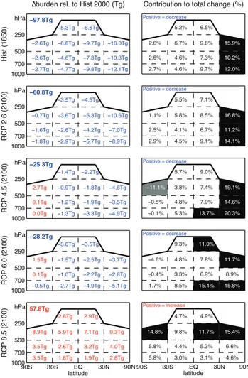
Figure 8 shows the mean model regional ozone burden changes relative to Hist 2000 for the Hist 1850 and the four RCP 2100 simulations, dividing up the troposphere in the same manner as Fig. 3b. The figure also indicates the frac-tion that each region contributes to the overall ozone change, i.e. highlighting asymmetries in the change. From Fig. 7, we see that the overall ozone burden change is negative for all of these simulations, except RCP8.5 2100. Based on the spread of model results, all of the regional burden changes are sig-nificantly different from zero.

For Hist 1850 and RCP2.6 2100 the burden change is negative for all regions, with the largest contribution to the change coming from the lower ozone precursor emissions in the NH extratropics compared to Hist 2000. Unlike for the other RCPs, stratospheric ozone recovery (e.g. Eyring et al., 2010) does not force an increase in tropospheric ozone for the SH upper troposphere, despite a 30 % increase in the total column ozone (not shown). However, an increase in strato-spheric influx is likely masking what would otherwise be stronger negative changes due to the precursor decreases (see Sect. 5.3). The SH extratropics makes a small contribution to the overall change for both the Hist 1850 and RCP2.6 2100 case.

The overall decrease for RCP4.5 2100 is about half of that between RCP2.6 2100 and Hist 2000, but is still largely dominated by the decrease in precursor emissions in the NH extratropics, with some contribution from the NH tropical lower troposphere. This overall decrease is countered by a relatively large increase in the SH upper troposphere, likely related to ozone recovery. The magnitude and patterns of ab-solute ozone changes are similar for RCP6.0, although the tropical upper troposphere makes more of a contribution to the overall change than in RCP4.5, in both absolute and rel-ative terms. For RCP8.5, ozone increases everywhere, al-though the largest contribution is from the 500 to 250 hPa pressure band.

Figures 9, 10 and 11 present information on the annual mean spatial patterns of ozone concentration changes, rela-tive to Hist 2000, for all the time slices, showing the absolute changes in zonal mean ozone, the tropospheric ozone column and surface ozone, respectively. Corresponding ozone differ-ences for the individual models can be found in the Supple-ment (Figs. S4–S6).

Concentrations for Hist 1850 are less than Hist 2000 ev-erywhere except the stratosphere (Fig. 9a), showing the im-pact of increased precursors (Fig. 1) and CFC-induced ozone depletion respectively. Relative decreases exceed 40 % for the column (Fig. 10a) and surface for NH mid-latitudes