Wives, husbands and wheelchairs: Optimal tax policy under gender-specific health

HAL Id: halshs-00575059

https://halshs.archives-ouvertes.fr/halshs-00575059

Preprint submitted on 9 Mar 2011

HAL is a multi-disciplinary open access archive for the deposit and dissemination of sci-entific research documents, whether they are pub-lished or not. The documents may come from teaching and research institutions in France or abroad, or from public or private research centers.

L’archive ouverte pluridisciplinaire HAL, est destinée au dépôt et à la diffusion de documents scientifiques de niveau recherche, publiés ou non, émanant des établissements d’enseignement et de recherche français ou étrangers, des laboratoires publics ou privés.

Wives, husbands and wheelchairs: Optimal tax policy

under gender-specific health

Marie-Louise Leroux, Grégory Ponthière

To cite this version:

Marie-Louise Leroux, Grégory Ponthière. Wives, husbands and wheelchairs: Optimal tax policy under gender-specific health. 2009. �halshs-00575059�

WORKING PAPER N° 2009 - 46

Wives, husbands and wheelchairs:

Optimal tax policy under gender-specific health

Marie-Louise Leroux

Grégory Ponthière

JEL Codes: H51, I12, I18, J14, J16

Keywords: Long term care, optimal taxation, preventive

health spending, gender differentials, old age dependency

P

-

S

E

L

’E

A

-

48, BD JOURDAN – E.N.S. – 75014 PARIS TÉL. : 33(0) 1 43 13 63 00 – FAX : 33 (0) 1 43 13 63 10

www.pse.ens.fr

CENTRE NATIONAL DE LA RECHERCHE SCIENTIFIQUE –ÉCOLE DES HAUTES ÉTUDES EN SCIENCES SOCIALES

Wives, Husbands and Wheelchairs:

Optimal Tax Policy under Gender-Speci…c Health

Marie-Louise Lerouxyand Grégory Ponthièrez

November 10, 2009

Abstract

We study the optimal taxation problem in an economy composed of two-person households (men and women), where agents in‡uence their own old-age dependency prospects through health spending. It is shown that the utilitarian social optimum can be decentralized by means of lump sum transfers from men to women, because women exhibit a higher disability-free life expectancy than men for a given level of health spending. Once self-oriented concerns for coexistence are introduced, the decentralization of the …rst-best requires also gender-speci…c subsidies on health spending aimed at internalizing the e¤ect of each agent’s health on the spouse’s welfare. In the presence of singles in the population, the optimal policy requires also a di¤erentiated subsidization of health spending for singles and couples. Finally, under imperfect observability of couples, the incentive compatibility constraints reinforce the need for subsidization of health spendings.

Keywords: Long term care, optimal taxation, preventive health spend-ing, gender di¤erentials, old age dependency.

JEL codes: H51, I12, I18, J14, J16.

The authors would like to thank Jacques Drèze, Dirk Van De Gaer, Pierre Pestieau and Erik Schokkaert for their helpful comments on this paper.

y_{CORE, Université catholique de Louvain. E-mail: Marie-Louise.Leroux@uclouvain.be} z_{Paris School of Economics and Ecole Normale Supérieure, Paris. E-mail:}

1

Introduction

A major challenge raised by the ageing of populations consists of the rising demand for long-term care (LTC) services, i.e. services necessary for persons who can no longer carry out daily activities such as eating, dressing, or bathing. Actually, whatever the scenarios on future dependency rates are, the number of dependents will grow in the next decades, making the LTC problem a major issue for policy makers.1 To give an idea, the European Union (2009) forecasts that the number of elderly dependents in the EU-27 will grow from 21 millions in 2007 to more than 44 millions in 2060.2 Such an evolution will stimulate the demand for LTC services, which may shift from informal care (provided by family or friends) to formal care (either at home or in nursing homes).3

Figure 1: Men and women old age dependency

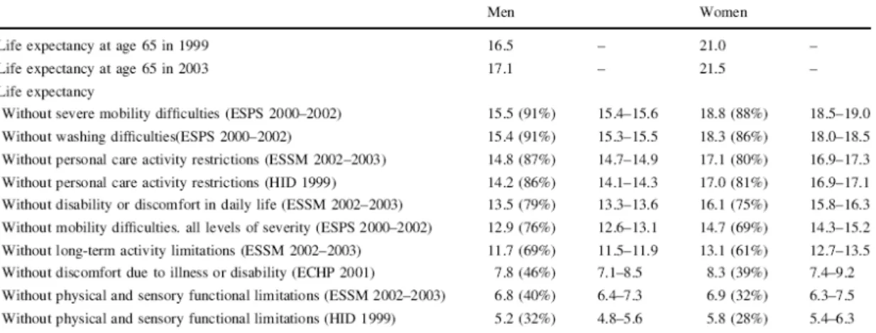
Besides its overall size, the LTC phenomenon involves also large gender dif-ferentials: women are, on average, far more subject to old age dependency than men are ceteris paribus.4 That gender di¤erential is illustrated, for France, by Table 1, which is taken from Cambois et al (2008). French women have, at age 65, a life expectancy that is 4.5 years longer than the one of men. Moreover, whatever the disability considered, women tend also to live longer without that disability. However, the period of dependency is longer, on average, for women. For instance, French women can expect, at age 65, to live about 3 years with

1

See Duee et al (2005) on the sensitivity of forecasts to old-age dependency scenarios.

2_{Note that this forecast, which assumes a (quite pessimistic) constancy of age-speci…c}

de-pendency rates, may tend to overestimate the size of the future number of dependents.

3

According to the EU (2009), 2/3 of the LTC services are currently provided informally in the EU-27, but that proportion is likely to shrink over time (see the EU for forecasts).

4

Note that there exist other sources of old age dependency di¤erentials. See for instance Pérès et al (2005) on the e¤ect of education di¤erentials on disability-free life expectancy.

washing di¢ culties, against only 1.5 years for men. Thus, while women have a longer life, these live also a longer period of dependency with LTC services.

Another important aspect of the LTC problem is the crucial role played by the marital status. Actually, whether a person belongs to a couple or not matters a lot for his health and survival prospects. For instance, Bouhia (2007) showed, on the basis of French data, that men aged between 50 and 60 years who are single face a mortality risk that is 40 % higher than the risk faced by men living in couples. That extra risk amounts to 70 % for women. Hence, the study of the LTC problem must take not only gender di¤erentials into account, but, also, the e¤ect of the marital status on the old-age dependency and survival.

Undoubtedly, the existence of large di¤erentials across people according to the gender and the marital status raises di¢ cult questions to policy-makers. The dilemmas could be summarized as follows. Should a government, in the light of those di¤erentials, subsidize men’s health spending in such a way as to make these live a longer autonomous life (like their wifes), or, on the contrary, should governments subsidize women’s health spending, in such a way as to reduce their - longer - period of dependency, or both? Moreover, should governments treat agents di¤erently, depending on whether they belong to a couple or not?

Although those questions become increasingly important for policy makers, little attention has been paid to those issues so far, as these lie at the intersection of two literatures that have not really merged so far.

On the one hand, recent articles in public economics have concentrated on the tax treatment of couples. In particular, several studies examined whether taxation systems should rely on joint or on individual taxation, in the cases where couples’members have di¤erent earning capacities and di¤erent elasticities of labour supply, in the presence or absence of household production (see Apps and Rees, 1988, 1999, 2007, Boskin and Sheshinski, 1983, Cremer et al., 2007 and Kleven et al., 2006). However, those studies did not consider the issue of long-term care, and could thus not examine the optimal taxation of LTC spending for agents who belong to a couple (or not), which is the topic of the present paper. On the other hand, there exists also a large literature on the demand and supply of LTC services (see Norton, 2000). Nevertheless, few papers consider the design of the optimal taxation policy under endogenous LTC demand. The few existing normative papers on LTC, such as Jousten et al (2005) and Pestieau and Sato (2008), have taken the dependency status of the elderly as something that is exogenously given, and, thus, could not discuss the optimal taxation of preventive LTC spending, i.e. spending that reduce the likelihood of old-age dependency. Moreover, those papers, which focused on the parent-child relationship, did not pay a particular attention to gender di¤erentials among the elderly, and to the impact of the marital status on agents’health. For instance, Jousten et al (2005) studied the optimal tax policy in an economy where households are composed of one dependent parent and one child, under heterogeneity on the altruism of children. More recently, Pestieau and Sato (2008) examined the optimal policy in an economy where some elderly become dependent, and where young adults di¤er in their productivity. Here again, the optimal policy was shown to depend on the available taxation instruments, as well as on the informational constraints

faced by governments, but there was no concern for heterogeneity among the elderly (either in terms of life expectancy or in marital status).

The goal of this paper is precisely to study the optimal tax policy in an economy where agents can in‡uence their future old-age autonomy, and where agents di¤er in gender and marital status. More precisely, we consider an econ-omy where agents can invest in preventive LTC spending, which can reduce the probability of old-age dependency, but where survival and dependency prospects are, ceteris paribus, varying with the gender and the marital status. As such, this paper complements the normative literature on LTC by introducing two sources of heterogeneity - the gender and the marital status - which, despite their impact on survival and autonomy, have remained so far largely ignored.

For that purpose, we develop here a two-period model, where the population is composed of two types of agents, i.e. men and women, whose di¤erent physio-logical characteristics lead to di¤erentials in survival and autonomy prospects. In that economy, men and women face an exogenous survival probability to the sec-ond period (which is larger for women than for men), and can in‡uence, through …rst-period health spending, gender-speci…c probabilities to be autonomous at the old age.5 _{For the conveniency of presentation, we will consider three versions} of that model, from the most simple to the most complicated.

In order to emphasize the consequences of gender-speci…c health, we focus, in a …rst stage, on a simpli…ed economy, where all men and women are singles, that is, an economy without welfare interdependencies. We describe the laissez-faire equilibrium in that economy where the disability-free life expectancy is endogenously determined by agents’ health investments. The social optimum and its decentralization through a tax and transfer policy are also examined.

In a second stage, we focus on an economy where all agents live in couples, and we introduce, at the level of agents’preferences, (1) a self-oriented concern for coexistence with the spouse; (2) an altruistic concern for the welfare of the spouse.6 In that framework, agents care not only about their own future survival and health, but, also, about the coexistence with their partner at the old age. As we shall see, that valuation of coexistence a¤ects the optimal policy, as it is a source of externalities. The government should make agents take into account the (partly ignored) e¤ect of their health investment on their partner’s welfare. In a third stage, we consider a more general economy, where some, but not all, agents live in couples. Even if it complexi…es the framework by adding two types of agents, the introduction of singles does not a¤ect the optimum subsidiza-tion of health spending. However, under imperfect observability of the marital status, incentive compatibility constraints reinforce the need for subsidisation. The optimal tax and transfer scheme also depends on the degree of altruism of individuals and on partition of the population into couples and singles.

Finally, it should be stressed that we will make, in the rest of this paper, the following assumptions, which allow us to focus on the speci…cities raised

5

Since we focus here on LTC, the assumption of exogenous (gender-speci…c) longevity prospects is made for conveniency. Naturally, longevity is probably as endogenous as old age dependancy. See Leroux et al (2008) on optimal policy under endogenous longevity.

by the two sources of heterogeneity under study. First, agents are standard expected utility maximizers.7 Second, individual temporal utility, which is state-dependent, is the same for men and women.8 Third, the government is, for the sake of simplicity, a classical utilitarian government.9

The rest of this paper is organized as follows. Section 2 presents the basic model with singles only, characterizes the laissez-faire, the social optimum, and its decentralization. Section 3 presents an economy composed of couples only, and shows how coexistence concerns a¤ect the optimal tax policy. Section 4 considers an economy where some persons form a couple, while others are single. Numerical simulations are carried out in Section 5. Section 6 concludes.

2

The basic model

2.1 Assumptions

Let us consider a population composed of two types of agents: men and women, indexed by M and F . All agents are endowed with an equal amount of resources w, and live as singles. Agents live, at most, two periods of life (of lengths normalized to one): the …rst period of life is lived for sure, while agents enjoy a second period of life with a probability of survival i, for i = M; F .10

Following the large literature on longevity di¤erentials across genders (see Vallin, 2002), we assume that

M < F

that is, men’s life expectancy, equal to 1 + M, is smaller than women’s life expectancy, equal to 1 + F.

Elderly agents who survived to the second period face a gender-speci…c risk of being autonomous, denoted by pi, for i = M; F: That probability of autonomy at the old age (conditional on survival) depends on health spending in …rst period

pi pi(mi)

where mi is the amount of his private health spending. We assume, as usual, p0_i(mi) > 0 and p00_i(mi_{) < 0 8i:}

Following demographic work on gender-speci…c probabilities, we assume that women face a higher age-speci…c probability of dependency11

pM(mM) = p (mM) pF (mF) = "p (mF) with " 1.

7

See Leroux and Ponthiere (2009) for an alternative modeling of health-a¤ecting choices.

8

However, that assumption does not prevent di¤erent health investments across genders, as di¤erent survival prospects are here formally equivalent to di¤erent degrees of impatience.

9

On the limitations of utilitarianism under unequal longevities, see Bommier et al (2009).

1 0_{Note that in Section 4, the survival probability will be di¤erentiated by marital status.} 1 1

While women face a higher dependency rate at a given age, these exhibit a higher disability free life expectancy, so that we assume that

1 + MpM(m) 1 + FpF(m) That assumption is equivalent to having M F".

Apart from these longevity and health di¤erences, men and women are, for simplicity, assumed to be identical on all other aspects. In particular, men and women have here the same productivity, w, and the same preferences.

Regarding the speci…cation of preferences, agents are assumed to be expected utility maximizers. As usual, lifetime welfare takes an additive form, but we assume nonetheless that temporal utility is state-dependent: the function u(:) denotes the utility of consumption under autonomy (i.e. good health), whereas the function v(:) denotes the utility of consumption under dependency (i.e. bad health).12 In the rest of the paper, we will assume that v (:) = u (:) L, where L represents a utility loss due to old age dependency.13

Assuming a zero interest rate and no pure rate of time preference, the ex-pected lifetime utility of an agent of type i = M; F can be written as14

Ui = u (ci) + i[pi(mi) u (di) + (1 pi(mi)) v (di)] (1) where ci, diare the consumptions in the …rst and the second periods respectively. First-period and second-period budget constraints are

ci w mi si

di Risi

For simplicity, we assume that individual savings si are invested in a perfect annuity market yielding actuarially fair returns (for di¤erent risk classes), so that Ri= 1= i.

2.2 Laissez-faire

An agent of type i = M; F solves the following problem

max u (w mi si) + i[pi(mi) u (Risi) + (1 pi(mi)) v (Risi)] First order conditions with respect to si and mi are, respectively,

iRi pi(mi) u0(di) + (1 pi(mi)) v0(di) = u0(ci) ip0i(mi) [u (di) v (di)] = u0(ci)

Under our assumption of a perfect annuity market ( iRi= 1) and replacing for the expression of v (:), we obtain

u0(ci) = u0(di) p0_i(mi) =

u0(ci) iL

1 2

As usual, we postulate u0(c) > 0, u00(c) < 0and v0(c) > 0, v00(c) < 0:

1 3_{This is done for simplicity, but other assumptions would not strongly a¤ect our results.} 1 4

Note, however, that the survival probability to the second period serves here as a natural discount factor.

Thus, consumptions are smoothed across time, for all agents.

We now compare the laissez-faire allocations of men and women. The above condition can be rewritten as

p0(mF) = 1 " u0(cF) FL p0(mM) = u0(cM) ML

Since men and women have the same productivity, they end up with the same lifetime income,

w = cF (1 + F) + mF = cM(1 + M) + mM

Using those three conditions and pF F > pM M (equivalently F" > M), we can show that the only possible solution consists in cF < cM and mM 7 mF. Our results are summarized in the following proposition.

Proposition 1 Provided the market for gender-speci…c annuities is actuarially fair, the laissez-faire allocation is such that

(i) cF = dF < cM = dM, (ii) mM 7 mF.

Thus, at the laissez-faire, women consume less than men in both periods. However, it is not obvious to see whether women spend more or less on their health than men. The reason behind that indeterminacy comes from the exis-tence of two e¤ects. First, women have smaller consumption in the second period, which reduces the incentive to invest in LTC. But, second, women face better survival prospects, which motivates more health investment ceteris paribus. The indeterminacy follows from those two opposite e¤ects.

2.3 Social optimum and decentralization

Let us now consider the problem of a utilitarian planner, who chooses consump-tions and health spending to maximize social welfare,

max ci, mi, di

i=F;Mnifu (ci) + i[pi(mi) u (di) + (1 pi(mi)) v (di)]g s.to W i=F;Mnifci+ mi+ idig 0

where ni is the proportion of agents of type i = M; F in the population, while W = i=F;Mniw is the total endowment of the economy. Under v (:) = u (:) L, the FOCs can be written as

u0(ci) = u0(di) p0(mF) = 1 " u0(c) FL p0(mM) = u 0_(c) ML

Thus, consumption is smoothed across times and individuals, cF = dF = cM = dM = c. Using pF F > pM M, we also now have mF > mM. Thus, at the social optimum, more resources should be spent on the health of women, as these enjoy, for an equal level of health spending, a higher disability free life expectancy than men, that is, a longer healthy life. In comparison with the laissez-faire, the indeterminacy does not hold here, as consumptions are equalized across agents, so that it is here more pro…table to invest in women’s health (as F > M).

It is straightforward to show that this social optimum can be decentralised through lump sum tranfers only, so as to equalise consumptions between indi-viduals. These net transfers, TF and TM are such that

TF = (1 + F) c + mF w > TM = (1 + M) c + mM w

Hence, the decentralization of this social optimum involves the transfer of re-sources from men to women. Our results are summarized in Proposition 2. Proposition 2 The …rst-best allocation yields:

(i) cF = dF = cM = dM = c, (ii) mF > mM.

Thus, if we assume a single source of heterogeneity - gender-speci…c survival and old-age dependency - the utilitarian optimum involves a redistribution of resources from men to women, as the latter, by having a better physiology, are a more direct way to raise social welfare.15 Note, however, that such a conclusion is premature, as the above analysis ignores an important aspect of the problem: in reality, men and women live generally in couples, so that welfare interdependencies exist. How would these a¤ect the optimal policy?

3

An economy of couples

To answer that question, this section studies an economy where all agents live in couples, and where no one stays single. For simplicity, all couples are assumed to be composed of a man and a women. In that economy, agents care not only about their survival and health, but, also, about the ones of the spouse.

3.1 The spouse’s utility function

In an economy of couples, individual preferences can hardly be represented by utility functions as simple as the ones used in the previous section. Members of a couple have the speci…city to care, in one form or in another, about their partner. The term "care" is quite general, and, as such, may lead to ambiguities, in the sense that there exist various ways to "care" about the partner. In our economy, each agent is assumed to care about his partner in two distinct ways.

First, an agent cares now not only about his own survival and health status (as above), but, also, about the survival and health status of his or her partner.

1 5

This is a consequence of utilitarianism, which, under additive lifetime utility, redistributes from short-lived to long-lived agents.

That concern is self-oriented or egoistic: the husband would like his wife to survive and be healthy if he survives, but this has nothing to do with the welfare (either consumption or health) of his wife. In other words, partners care about the survival and health of their spouse just to avoid loneliness or care-provision. Second, an agent cares also about what his or her partner feels, that is about her welfare. This constitutes another form of concern, which is distinct from the previous one, as this involves what is usually referred to as "pure" altruism. A major distinction with respect to the previous concern is that, in the present case, the interest of the agent in his or her partner is not conditional on his / her own survival, contrary to what prevailed under the …rst motive.16

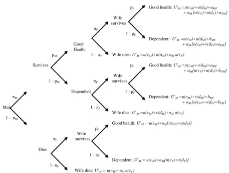
Let us see how those two distinct forms of concerns for the partner can be in-troduced within our model. To keep the model as simple as possible, we assume that agents are, as above, expected utility maximizers. Moreover, for simplicity, individual utility in each state is additive with respect to the self-oriented co-existence concern and the altruistic concern. Under those assumptions, agents face a lottery, whose form is illustrated on Figure 2, for the case of men. That lottery includes 9 distinct scenarios: in the case where both the husband and the wife survive, there are four possible scenarios in terms of old-age dependency; in each case where only one member of the couple becomes old, there are 2 dis-tinct scenarios in terms of old-age dependency; …nally, in the case where no one reaches the old-age, there is a unique scenario, as old-age dependency does not matter in that case. This makes a total of 4 + (2 x 2) + 1 = 9 outcomes.

Figure 2 presents the utility assigned to each outcome by men. The parameter aM F denotes the (self-oriented) utility gain, for the man, from coexisting with a healthy wife (whatever he is autonomous or not); bM F denotes the utility gain, for the man, from coexisting with a dependent wife; aF M and bF M are the corresponding utility gains for women. Alternatively, the parameter M captures the extent to which a husband is sensitive to his wife’s welfare.17

Throughout this paper, we assume that each agent prefers, from a purely egoistic perspective, to coexist with a healthy person than with an unhealthy person, and prefers coexistence with an unhealthy person to loneliness. Hence

0 < bM F < aM F 0 < bF M < aF M

Those parameters are assumed to be independent from the agent’s own health.18

1 6

However, agent’s altruistic concern for the other concentrates here on the private (i.e. self-centered) part of his welfare. Alternatively, taking the whole welfare into account would yield a recursive welfare. Given that this more complex modeling would not yield additional insights for the issue at stake, we will focus here on the simple altruistic form proposed above.

1 7_{Note that, if the man was purely self-oriented, we would have}

M equal to zero, and, as a

consequence, the husband would be totally indi¤erent between the last three branches of the tree, where he did not survive the …rst period. Indeed, if there is no altruism, then in case of death the man does not care about the survival and/or health status of his wife at the old age, so that the number of relevant scenarios is reduced to 6.

1 8

This modelling of agents’concerns for coexistence is made for the sake of analytical conve-niency. It is likely that, in reality, the welfare gain, for an agent, from coexisting with a healthy rather than an unhealthy partner (e.g. for men: aM F bM F) may depend on whether he is

pF Good health: U

c

M =u(cM)+u(dM)+aMF

+ M[u(cF)+u(dF)+aFM]

Wife survives F 1 - pF Dependent: Uc M =u(cM)+u(dM)+bMF

Good + M[u(cF)+v(dF)+aFM]

Health

pM 1 - F Wife dies: U

c

M =u(cM)+u(dM)+Mu(cF)

Survives pF Good health: U

c M =u(cM)+v(dM)+aMF + M[u(cF)+u(dF)+bFM] Wife 1 - pM F survives Dependent 1 - pF M Dependent: UcM =u(cM)+v(dM)+bMF + M[u(cF)+v(dF)+bFM] . Man 1 - F Wife dies: Uc M =u(cM)+v(dM)+Mu(cF) 1 - M Good health: Uc

M = u(cM)+M[u(cF)+u(dF)]

pF Wife F survives Dies 1 - pF Dependent: Uc M = u(cM)+M[u(cF)+v(dF)] 1- F Wife dies: Uc M = u(cM)+Mu(cF)

Figure 2: Men’s lottery under sel…sh coexistence concerns and altruism

Moreover, no particular restriction is imposed on the altruistic parameters M and F, except that these are non-negative, and less than unity:

0 M 1

0 F 1

The parameter i2 [0; 1] 8i = M; F can be interpreted as the degree of altruism of an agent i belonging to a couple. The idea behind that restriction is that members of a couple care positively about the welfare of the other (i.e. non-negativity of i), but do not give more weight to the welfare of their partner than to their own welfare (i.e. i 1). In the most extreme case, they behave as an "ideal couple" (i.e. M = F = 1), in which decisions coincide with what a unique person would decide.19 But in general, we will observe M < 1 and F < 1, that, is, an imperfect internalization, by the agents, of the impact of their decisions on the other’s welfare.

Under expected utility hypothesis and additive temporal utility in coexistence and altruistic concerns, the preferences of a man belonging to a couple can, after simpli…cations, be represented by the following utility function,

U_Mc (cM; dM; mM) = UM+ M FbM F + M FpF (mF) M

+ M[UF + F MbF M+ F MpM(mM) F] (2) himself dependent or autonomous. Taking that di¤erence into account would demultiply the number of parameters of interest, and this is why do not take that di¤erence into account here.

1 9

That special case is an occurence of a perfect harmony, where each member of the couple treats the other as he would treat himself.

where UM, UF are de…ned by (1). The superscript c in UMc stands for couple concerns. In order to simplify notations, we rede…ne the net bene…t for a woman of having an autonomous husband as F aF M bF M and the net bene…t for a man of having an autonomous wife as M aM F bM F.

Hence, the utility function of a man belonging to a couple is the sum of four terms. The …rst term is the utility of a single individual, as in the previous section. The second part corresponds to the welfare from coexisting with his wife, i.e. M FbM F+ M FpF(mF) M, where M FbM F represents the pure utility from coexistence, independently from the health status of the wife (the product M F being the expected coexistence time at the old age).20 The third term represents the welfare gain, for the husband, from coexisting with a healthy wife (whatever he is himself healthy or not). That expression depends on the expected coexistence time with a healthy wife at the old age - i.e. M FpF(mF) - and on the utility gain associated to the autonomy of the wife, i.e. M. Finally, the last term in (2) accounts for the fact that the utility of a man belonging to a couple depends also on the utility of his wife. Given that this depends on the probability of the husband to be autonomous, the latter is going to take this into account when choosing his health spendings, mM. The extent to which he takes it into account depends on the value of M.21

Similarly, for women, the expected lifetime utility becomes here: U_Fc (cF; dF; mF) = UF + F MbF M + F MpM(mM) F

+ F[UM + M FbM F + M FpF(mF) M] (3) In this extended model, the man’s utility is, because of coexistence, a function of the woman’s probability of autonomy pF(mF), while the woman’s utility is a function of the man’s probability of autonomy p(mM). Hence, except in the case where the health status of the coexistent does not matter (i.e. i = 0 for i = F; M ), we are in presence of some externalities. Under i < 1, that is, under an imperfect couple, agents, when choosing how much to spend on health, tend to underestimate the externality their health status creates on the welfare of their partner. Hence, under a decentralized decision of individual health investments, the laissez-faire is likely to be suboptimal.22

3.2 Laissez-faire

Let us now solve the laissez-faire equilibrium. Note that even if agents form a couple, their preferred bundle is not, under i 6= 1, equivalent to the one obtained from the maximisation of a couple’s utility under a single budget constraint (this will rather correspond to the …rst-best equilibrium). We consider here a

2 0_{On the measurement and evolution of joint life expectancies over time, see Ponthiere (2007).} 2 1

For instance, if M = 1, the man perfectly estimates the impact of his health spending on

the welfare of his spouse, while if M = 0, he does not see this e¤ect at all. 2 2

Of course, coexistence would not be a source of externalities in the case of a perfect couple (i.e. M = F = 1). In that case, individual decisions coincide with the ones taken by a unique

decision maker, and all variables would be chosen in such a way as to maximize household’s welfare (no intracouple externality).

couple who would fully behave non-cooperatively. Quoting D’Aspremont and Dos Santos Ferreira (2009), the type of couple we consider here is one that acts as an “independant management system in which each spouse keeps his / her own income separate and has the responsability for di¤erent items of household expenditure”.

For a man, the problem consists in choosing consumptions and health spend-ing so as to maximize (2) ;

U_Mc (cM; dM; mM; mF) = u (cM) + M[pM(mM) u (dM) + (1 pM(mM)) v (dM)] + M FbM F + M FpF(mF) M

+ M[UF + F MbF M + F MpM(mM) F] subject to the resource constraints

cM w mM sM

dM RMsM

Rearranging …rst-order conditions yields u0(cM) = u0(dM) p0(mM) =

u0(cM) ML + M F M F

In comparison to Section 2.2, the second term in the denominator of the condition on mM has to do with man’s altruism. The higher the altruistic concern is (i.e. the higher M is), the higher the health investment is ceteris paribus. Note, however, that the strength of that term depends not only on the welfare assigned by woman to the man’s health, F, but, also, on the expected future coexistence time, F M. Indeed, it is only to the extent that the wife survives and, of course, that the husband survives, that the man’s health decision matters for the women.

As for women, the problem is to maximise (3) subject to

cF w mF sF dF RFsF and obtain u0(cF) = u0(dF) p0(mF) = 1 " u0_(cF) FL + F M F M

Those conditions are symmetric to the ones describing the husband’s decisions. Finally, note that the conditions characterizing mM and mF di¤er from the ones in the basic framework (see section 2.2), by a term M F i j. This is due to the fact that an individual belonging to a couple now cares for the welfare of his partner, which itself depends on his probability of being in good health (through the utility obtained from coexistence). If i < 1, the individual partly internalizes this e¤ect of his health expenditure on the welfare of his/her partner. As we shall see in the next section, depending on the magnitude of i, this positive externality may not be completely internalised by the individual, so that the laissez-faire can be ine¢ cient. Our results are summarized below.

Proposition 3 Under coexistence and altruistic concerns, the laissez-faire allo-cation is such that:

(i) ci= di _{8i 2 M; F ,}

(ii) mi is increasing in the altruistic parameter i, and in the self-oriented coexistence gain of the spouse _{j, for i; j 2 M; F:}

Note that it cannot be said a priori whether women tend to invest more or less in their health than men, as this depends on various preferences parameters of both women and men.

3.3 First-best

Let us now consider the problem of a utilitarian social planner under the new speci…cation of individuals’utility. As this is well-known in the LTC literature (see Jousten et al, 2005), the existence of altruistic concerns raises some di¢ cul-ties, as it is not straightforward to see how altruistic concerns should be taken into account by the social planner. Actually, various possibilities exist.

First, one can assume that the social welfare function should rely on the actual altruistic coe¢ cients, i.e. M and F, whatever these are equal or not, and whatever the consequences are.

Second, one could assume that the social planner should not take altruistic concerns into account, and should …x all altruistic coe¢ cients i equal to zero when de…nining the objective function. Such a position can be defended on the grounds that altruistic preferences should be regarded as irrelevant for the distribution of income (see Hammond, 1987).

A third position consists in claiming that altruistic concerns should be taken into account by the social planner, but not in their existing, imperfect forms, but, rather, under an ideal form, i.e. should be …xed to 1. The underlying idea is that the planner should do as if couples were “ideal” couples, in which each member would be able to anticipate perfectly the impact of his actions on the welfare of his spouse.23

Throughout this section, we will not adhere to the …rst position, as it seems unfair to make the social optimum dependent on the actual altruistic parameters. It is indeed hard to see why more altruistic persons should be favoured for their altruism, by receiving more resources. However, we will not choose here between the second and the third solutions. We will, on the contrary, impose i= in the planner’s objective function. Depending on whether one adheres to the second or the third position, one will be free to …x = 0 or = 1.

Thus the problem of the social planner is now

max nMU_Mc (cM; dM; mM; mF) + nFU_Fc (cF; dF; mF; mM)

s.to W nM_fcM + mM + MdMg nFfcF + mF + FdFg 0

2 3_{One can justify the planner’s attitude through "old" or "new" paternalism. Old paternalism}

would amount to say that, by …xing i= 1, the social planner expresses his view that

individ-uals, because they are part of a couple, should treat their partner exactly like themselves. New paternalism, on the contrary, would regard i < 1as a kind of interpersonal myopia (rather

than intertemporal myopia as usual). Agents would behave according to i < 1, but would

where we posit M = F = in UMc and UFc. In such a case, we show that, under ₆₌ M; F, the laissez-faire equilibrium is not optimal.

By assumption, in a society where there are only couples, we have nM = nF = n. In the Appendix, we show that FOCs can be rearranged as

u0(cM) = u0(dM) = u0(cF) = u0(dF) = (1 + ) (4) p0(mM) = u0(c) ML + F M F (5) p0(mF) = 1 " u0_(c) FL + M F M (6) where is the Lagrange multiplier associated with the resource constraint. As in the initial …rst-best, consumptions should be equalized across agents and periods, cF = cM = dM = dF = c. On the opposite, whether mM 7 mF now depends on whether F 7 M. If the extra net bene…t the man gets from coexistence with a healthy partner is larger than the one of the woman (i.e. M > F), then mF > mM with no ambiguity. The social planner encourages more health expenditures of the woman, both because she creates a higher positive externality on her husband and because she is more likely to survive (so that it is more pro…table to invest on her autonomy). On the contrary, if M << F (i.e. the bene…t for a woman of having an autonomous husband is much bigger than the bene…t for a man of having an autonomous wife), it might be the case that mF < mM.24

The social optimum involves higher health spendings than under the laissez-faire. This is related to the non-internalized (self-oriented) coexistence concerns. In the laissez-faire, agents underinvest in their health, as they internalize only imperfectly the e¤ect of their decisions on the other’s (self-oriented) welfare. Moreover, the extent of underinvestment in health depends not only on how i di¤ers from 1 (i.e. full internalization), but, also, on the joint life expectancy of the couple, and on the size of the coexistence bene…t for the spouse (i.e. the magnitude of the externality). Our results are summarized in Proposition 4. Proposition 4 At the …rst-best optimum, we have, whatever is:

(i) cF = cM = dM = dF = c, (ii) mM 7 mF,

(iii) provided i< 1, we have mi > mLFi , 8i = F; M:

Note that, in comparison with the laissez-faire, we have a higher level of health spending at the …rst-best, whatever we …x to 0 or 1. This somewhat surprising result comes from the fact that, at the …rst-best, counting each men or women once or twice does not matter, as long as all members of couples are counted in the same way, which is the case under either = 0 or 1. To put it di¤erently, the externality does not depend on whether the social planner …xes

2 4_{This is so because the husband creates, in that case, a very large positive externality on}

the woman (as she really enjoys living with a healthy partner); this counterbalances the fact that he has a smaller survival probability than her.

the altruistic weight to 0 or 1, as this is related to the egoistic part of one’s welfare. Hence it should not be surprising that the level of does not matter for the extent of underinvestment in health.

3.4 Decentralisation of the …rst-best

We now study how to decentralise the above optimum through a tax-and-transfer scheme. In the following, we assume that instruments available for the social planner are a tax on savings, i, on health expenditures, i, and a lump sum transfer, Ti. We still assume that the annuity market is actuarially fair so that Ri = 1= i at equilibrium. The problem of a man is then:

max sM, mM U_Mc = UM + M FbM F+ M FpF (mF) M + M[UF + + F MbF M + F MpM(mM) F] s.to cM w mM(1 + M) sM(1 + M) + TM dM RMsM

First order conditions are u0_(dM) u0_(cM) = 1 + M (7) p0(mM) = u0_(cM) ML + M F M F (1 + M) (8)

Using the same procedure, we obtain similar …rst order conditions for women, u0(dF) u0_(cF) = 1 + F (9) p0(mF) = 1 " u0(cF) FL + F M F M (1 + F) (10)

Comparing these equations with the ones of the …rst-best (4, 5, 6), we get the following result.

Proposition 5 In an economy made of couples only, implementing the …rst-best optimum only requires taxes on health,

M = (1 M) 1 + L= F F < 0 F = (1 F) 1 + L= M M < 0 and lump-sum transfers TF and TM:

Note that, here, we do not need to tax savings, F = M = 0 and that the direction of transfers depends on M and F. If M > F, TF > TM; otherwise it is ambiguous.

Men and women’s health spending should be subsidized, as they create a positive externality on each other, through individual self-oriented concern for

coexistence. The subsidy on health spending i depends on the form of coexis-tence concerns, i.e. on j, and on the degree of altruism, i. If, for instance, the man (resp. the woman) perfectly internalizes his (her) in‡uence on his spouse welfare, that is, if M = 1 (resp. F = 1), no subsidy is required and M = 0 (resp. F = 0). In that case, agents act exactly as the ideal couple, and equally care about their welfare and the one of their partner. The decentralisa-tion requires only lump sum transfers (to operate redistribudecentralisa-tion between men and women).

If, on the contrary, i < 18i, distortionary taxation is necessary and i < 0 depends on j. To understand this, assume now that 0 < M = F < 1, so that both members of the couple equally underestimate their in‡uence on the other’s welfare. If F M, we obtain that j Mj j Fj. In this case, health spending of the man should be more subsidized, …rst, because the woman is more likely to bene…t from a autonomous husband ( F > M) and second, because the net bene…t she obtains from him being autonomous is higher.25 _{Otherwise, we} may have j Mj 7 j Fj. If, for instance, the bene…t the woman gets from having her husband autonomous is much lower than the bene…t the husband gets from having his wife autonomous, i.e. F << M, one may have j Mj < j Fj.

4

An economy with singles and couples

Whereas Section 3 assumed that all men and women care about the coexistence with their partner, this modelling was a simpli…cation of reality, as some men and some women are actually single. A more realistic description of reality should involve men and women organized in couples or not, that is, a society where some agents have coexistence concerns, while others have not. However, whether men and women are single or not is not neutral as far as health is concerned. As shown by Bouhia (2007), men aged between 50 and 60 years who are single face a mortality risk that is 40 % higher than the risk faced by men living in couples. That extra risk amounts to 70 % for women.26

To do justice to those concerns, let us now assume that the society is consti-tuted of both single individuals and married ones, denoted by the superscripts s for singles and c for couples. For simplicity, the structure of the society is here taken as …xed by individuals (no possibility of divorce) and by the social planner.27 We have ns_M and ns_F the numbers of men and women who are single, and nc_M = nc_F = nc the number of couples.

Following demographic studies, we now assume: s

M < cM s

F < cF

2 5_Having

M < F reinforces the gap between j Mj and j Fj. 2 6

It should be stressed, however, that the mortality di¤erentials between singles and couples tend to vanish as the age goes up. Moreover, agents who never lived in couples are an exception, in the sense that these face a lower mortality risk at high ages.

This means that single persons are, ceteris paribus, characterized by lower survival prospects than married persons. This speci…cation captures the fact that merely coexisting with a partner reduces the negative consequences of accidents (e.g. call for an ambulance), and promotes also a healthy way of life.28

4.1 First-best

4.1.1 Centralised solution

Provided he takes the family structure as …xed, the social planner solves the following problem: max nc[U_Mc (cc_M; dc_M; mc_M; m_Fc) + U_Fc (cc_F; dc_F; mc_F; mc_M)] +ns_MUM(csM; dsM; msM) + nsFUF (csF; dsF; msF) (A) s.to W n s MfcsM + msM + sMdsMg nsFfcsF + msF + sFdsFg nc_fcc_M+ mc_M + c_Mdc_M + cc_F + mc_F + c_Fdc_Fg 0

where lifetime utilities U_ic are de…ned by (3) and (2), where we substituted for c

M and cF and Ui are de…ned by (1) where we substituted for si.

As in Section 3, we assume that M = F = in UMc and UFc, because there is no consensus on the altruistic parameters that should be used by the social planner. As we already mentioned, assuming that M = F = = 1 accounts for the fact that the social planner would like to model an ideal couple, in which each member treats his partner exactly like himself. In that sense, public intervention is justi…ed to allocate resources as if we had an ideal couple, in which each member had the same bargaining power. This solution can be obtained by …xing to 1. However, such a modelling has here a serious drawback, as it penalizes singles. Clearly, there is, in the objective function of the social planner, something like a double-counting of a couple’s members as compared to single individuals. Given that agents are not necessarily responsible for being single, this double-counting of spouses may not seem fair. Thus, to avoid this, one could assume M = F = = 0. We will compare those two social optima in this section. As we shall see, this does not change our results on the optimal health spending, but it will have consequences on the optimal consumptions.

2 8_{Because we did not …nd any evidence that the marital status also in‡uences the probability}

of autonomy, we keep, for simplicity, our initial formulations for pM(:)and pF(:), and do not

The …rst-order conditions of the social planner’s problem are:29 u0(cc_M) = u0(cc_F) = u0(dc_M) = u0(dc_F) = (1 + ) = u 0_(cc_{) (11)} u0(cs_M) = u0(cs_F) = u0(ds_M) = u0(ds_F) = = u0(cs) (12) p0(mc_M) = u 0_(cc₎ c ML + cF cM F (13) p0(mc_F) = 1 " u0(cc) c FL + cM cF M (14) p0(ms_M) = u 0_(cs₎ s ML (15) p0(ms_F) = 1 " u0(cs) s FL (16) As above, consumptions are still equalized across periods and between women and men of the same group (i.e. single or couple). However, consumption may be here di¤erent for individuals with di¤erent marital status, depending on the value of the parameter . If, for instance = 0, consumption is smoothed between groups, and all individuals obtain the same level of consumption: cc = cs. However, if equals 1, consumption levels in all periods are larger for a member of a couple than for a single individual: cc _{> c}s_{. This is due to the fact} that the consumption of a member of a couple creates a positive externality on the welfare of the other member of the couple, so that the planner wants to favor it, through higher consumption levels.

Health expenditures are now di¤erentiated not only with respect to gender, but, also, with respect to the marital status. As before, we have ms_M < ms_F and mc

M < mcF for reasonable di¤erences between F and M. Additionally, health spending of agents who belong to a couple should now be higher than the ones devoted to singles, that is, ms_F < mc_F and ms_M < mc_M.30 This is the result of the positive externality they create on their partner. This e¤ect is also reinforced by the fact that members of a couple have, ceteris paribus, a higher life expectancy than single individuals, so that they are more likely to bene…t from these health investments. It is thus optimal to put more resources on them, so as to increase the probability of the good health scenario in the future. Those results are independant of the value of i, since it does not enter explicitly into equations (14) to (16). Our results are summarized in Proposition 6.

Proposition 6 The …rst-best optimum is such that:

(i) consumption is smoothed across periods and between individuals with the

2 9_{See Appendix B for calculations.} 3 0

Assuming a probability of autonomy that depends on the marital status would only modify the size of (mc

M msM). In this case, if the probability of autonomy is smaller (resp. greater)

for singles than for couples (for the same level of m), this would decrease (resp. increase) ms

M relative to mcM and thus, increase (resp. decrease) the gap between health expenditure of

same marital status,

cc = cc_M = dc_M = cc_F = dc_F and cs = cs_M = ds_M = cs_F = ds_F. and if = 0, cc = cs, while if > 0, cc > cs,

(ii) health spending are lower for men than for women mi_M < mi_{F 8i = s; c, and} for singles than for couples, ms_i < mc_{i 8i = F; M.}

To sum up, playing with the value of has consequences on consumptions only. Note that, a priori, there is no obvious reason for preferring = 1 over = 0. Yet, as shown below, this choice has consequences on the size of redistribution from single to couples.

4.1.2 Decentralised solution

As before, we assume that the optimum can be decentralised using the following instruments, which may be di¤erentiated by gender, i = F; M and by marital status, j = s; c: a tax on savings, j_i, a tax on health spendings, j_i and lump sum transfers, T_ij. Proposition 7 shows our results.31

Proposition 7 In a society where there are couples and singles, the decentrali-sation of the …rst-best optimum only requires to subsidize couples’ health expen-diture: c M = cF = sM = sF = 0 (17) s M = sF = 0 (18) c M = (1 M) 1 + L= c_F F < 0 (19) c F = (1 F) 1 + L= c_M M < 0 (20)

Lump sum transfers from men to women and from singles to couples are also necessary:

T_Mi < T_Fi _{8i = s; c} T_js < T_jc _{8j = F; M}

As in Section 3, there is no tax on the savings and on the health expenditures of single agents, since they do not create any externality. However, there is a subsidy on couples’s health spendings, in order to internalize the (self-oriented) coexistence externality. As in Section 2, c_i depends on how much the agent in a couple cares for his partner, i, on the coexistence bene…t the individual creates on his partner if autonomous, j and on the probability of his partner to e¤ectively enjoy this bene…t, c

j.

To see these e¤ects, assume …rst that i = 18i, so that the utility function of agent i corresponds to the one taken by the planner. In this case, no tax or subsidy on health is required, as individuals perfectly internalize their impact on partners’welfare. Only lump sum transfers are needed. Let us now assume that partners equally care about the welfare of others, i.e. M = F, and that the coexistence bene…ts are equal, i.e. F = M. In this case, the subsidy on the man’s health spending is higher, because c_F > c_M, that is, the probability that the woman actually bene…ts from the coexistence (with an autonomous partner) externality is higher. This e¤ect is ampli…ed if the bene…t from healthy coexistence is larger for the woman than for the man, i.e. if F > M.

Regarding the direction of transfers, we obtain that the …rst-best optimum is achieved by means of lump sum transfers from men to women (independently from their marital status) and from singles to couples, as we have:

T_Mj = cj(1+) j_M+ mj_M w < T_Fj = cj(1+) j_F + mj_{F w 8j = s; c,} and T_is= cs(1+) s_i + ms_i w < T_ic = cc(1+) c_i + mc_{i w 8i = M; F .} Note that T_Mc < T_Fc holds for reasonable di¤erence between F and M while for other categories, no condition is required. If the planner considers that = 0, we have cs = cc, while if = 1, we have cs < cc. Hence, transfers should be higher if = 1 than if = 0, because consumptions are also di¤erentiated according to the marital status.

4.2 Asymmetric information

In this section, we assume that the social planner cannot observe with certainty whether individuals belong to a couple or whether they are single.32 _{In the} previous subsection, we showed that the health spendings of a couple are al-ways larger than the ones of a single, ms_i < mc_{i 8i = M; F and that if} = 1 (or 0), consumptions of a couple should be also larger than for a single (resp. equal). Thus, if the social planner cannot observe the marital status of agents and proposes the …rst-best bundles, single individuals have always interest in claiming to be part of a couple, even though they have no coexistence concerns and do not care about the welfare of a partner. In such a case, we may actually expect false couples to be declared, just to bene…t from higher health spendings (and consumption levels), which would be a social waste in the absence of real coexistence concerns. In this subsection, we account for that asymmetry of in-formation and design an allocation, which prevents any type from pretending to be of the other type.

The second-best problem of the social planner corresponds to problem (A), to which we add two incentive constraints:

UM(cs_M; ds_M; ms_M) UM(cc_M; dc_M; mc_M) UF(cs_F; ds_F; ms_F) UF(cc_F; dc_F; mc_F)

These two constraints simply require that single individuals (either men or women) are always better-o¤ with their single’s bundle than with the bundle of a couple’s member.

Depending on the ability of the government to double-check the marital sta-tus of its citizens (i.e. for the husband and the wife) or not, and on the ability of agents to play cooperatively or not when reporting their marital situation, four cases can arise. These cases are summarized in the table below, where F and M denote the Lagrange multipliers associated with the two incentive compatibility constraints.

Agents Governement

single check double check

Play non-cooperatively _M > 0; _F > 0 M > 0; F = 0 or _M = 0; _F > 0 Play cooperatively _M > 0; _F > 0 _M > 0; _F > 0

If the government can only single check (because, for instance, of atomicity) and if agents do not play cooperatively (no transfers are possible), then none of the two incentive constraint is redundant, as a single person can always pretend to be married, and lie on its own (given the absence of double-check). If the gov-ernment can double-check, and if agents play non-cooperatively, then one incen-tive constraint becomes redundant.33 If the government can only single-check, but agents play cooperatively, then the two incentive constraints are needed: otherwise, if only one is binding, monetary transfers from one person to another could induce the formation of a false couple. The same would be true even if the government can double-check.

In the rest of this subsection, we abstract from the special case where the government can double-check the marital status of citizens, and where agents cannot play cooperatively. As a consequence, we shall have _F > 0 and _M > 0. In the Appendix, we solve the problem and show that …rst order conditions can

3 3_{Note that, in an economy where the government could double-check the marital status of}

be rearranged as u0(ds_M) u0 _cs M = 1 (21) u0(ds_F) u0 _cs F = 1 (22) p0(ms_M) = u 0_(cs M) s ML (23) p0(ms_F) = u 0_(cs F) " s FL (24) u0(dc_M) u0 _cc M = 1 M (1+ )nc 1 M sM (1+ )nc c M (25) u0(dc_F) u0 _cc F = 1 F (1+ )nc 1 F sF (1+ )nc c F (26) p0(mc_M) = u0(cc_M) 1 M (1+ )nc c ML 1 M sM (1+ )nc c M + c F cM F (27) p0(mc_F) = 1 " u0(cc_F) 1 F (1+ )nc F c FL 1 F sF (1+ )nc c F + c F cM M (28)

As before, we assume that the altruism parameter can be either 0 or 1 and compare the implications these assumptions have.

We …nd no distortion at the top, i.e. single individuals face the same trade-o¤s as in the …rst-best. Consumption should be smoothed across time for single men and women. However, in the second best, there is no reason for consumption to be equalised between single men and women: this is due to the introduction of the two incentive constraints. This also implies that we cannot tell whether ms_M 7 ms_F.

As for the couples, consumption trade-o¤s are now distorted downwards and we …nd that dc_M > cc_M and dc_F > cc_F. In comparison to the second best, the social planner encourages second-period consumption for agents belonging to a couple, as a way to discourage singles from mimicking them. Indeed, if a single agent pretended to be in couple, he would obtain too high a level of second-period consumption given his survival probability (we have that s_M < c_M).

Note that this reasoning applies also to health expenditures. As compared to the …rst-best trade-o¤, the right hand sides of (27) and (28) are smaller, so that health spending are encouraged for men and women living in a couple (i.e. mc;F B_i < mc;SB_{i 8i). As before, the social planner provides more health spending} to those individuals as a way to discourage singles from pretending to belong to a couple. For them, it is not worth investing that much in health, as they face a lower probability to survive in the second period than agents in couples (and this would be to the detriment of their …rst-period consumption).

Finally, the second-best distortion for couples is greater when = 1 than when = 0.34 This is linked to the introduction of the incentive constraint: if = 1, the utility of a true member of couple is counted twice in the objective function, while the utility of single individual pretending to belong to a couple is only counted once in the incentive constraint.35 Thus, the double counting e¤ect mentioned earlier now appears also through the incentive constraint. Thus, in (25) and (26), the gap between two-period consumptions of a couple is smaller when = 1 than when = 0 (as u (:) is increasing and concave). Similarly, in (27) and (28), the level of health spending is smaller ceteris paribus if = 1 than if = 0.

Finally, we study how to decentralise the second-best. In the Appendix, we derive the optimal second-best levels of j_i and j_i, with i = M; F denoting the gender and j = c; s denoting the marital status.

Proposition 8 Under asymmetric information, the decentralisation of the op-timum requires only to subsidize couples’ savings and health expenditure:

s M = sF = sM = sF = 0 c M = 1 M (1+ )nc 1 M M (1+ )nc c M 1 < 0 c F = 1 F (1+ )nc 1 F F (1+ )nc c F 1 < 0 c M = (L + M c_F F) 1 _{(1+ )n}M c L 1 M M (1+ )nc c M + c F F 1 < 0 c F = (L + c_F c_M M) 1 _{(1+ )n}F c F L 1 F F (1+ )nc c F + c M M 1 < 0

As in the …rst-best, single individuals (independantly of their gender) are not taxed. On the contrary, individuals living in couple now face a subsidy on second-period consumption, so as to solve the incentive problem. Regarding the subsidy on health expenditure, its level is higher than in the …rst-best as there are now two e¤ects playing in the same direction. First, this subsidy aims at internalizing the positive coexistence externality and second, it is used as a way to prevent singles from mimicking couples. The subsidies (either on savings or on health expenditure) also depend on the parameter chosen by the social planner, through the incentive term. If = 1, the subsidy tends to be smaller than if = 0, ceteris paribus.36 Note that lump sum transfers depending on the gender and on the marital status are also likely to take place. However, their

3 4

To see this, compare the right hand sides of expressions (25) (28)when = 1and when = 0. These expressions are bigger in the former than in the latter case.

3 5_{If = 0, we obtain the usual distortion factor, 1}

M=n c_. 3 6

As we show in the numerical section, susbsidies can be smaller if = 0. This reverse result is obtained because the _is are also modi…ed.

direction is ambiguous (since we can only imperfectly rank consumptions and health spendings across individuals).

5

A numerical illustration

5.1 Calibration

Let us now illustrate our …ndings by means of some numerical simulations. For that purpose, we shall assume that temporal welfare takes a simple CES form:

u(ci) = c1_i 1

where is the inverse of the elasticity of intertemporal substitution (here equal to the coe¢ cient of relative risk aversion).37 We assume = 0:83 as a benchmark case (see Blundell et al, 1994).

The old-age dependency for men and women is modelled by means of func-tions that are increasing and concave in health spending:

pM(mM) = AmM

1 + AmM pF(mF) = " AmF

1 + AmF where A is a positive constant.

In order to calibrate the parameters A and ", we need to consider the data on life expectancies and healthy life expectancies for men and women. On the basis of Table 1 for France, and assuming an initial age of 25 years and a length of period of 40 years, we have a life expectancy for men at age 65 equal to M = 17:1=40 = 0:4275 period, and a life expectancy at age 65 for women equal to F = 21:5=40 = 0:5375 period.

Healthy life expectancy at age 65 for men is MpM = 15:5=40 = 0:3875, while for women it is FpF = 18:8=40 = 0:47. Therefore, under M = 0:4275 and F = 0:5375, we have pM = 0:906 and pF = 0:874. Hence, assuming that health spendings are equal for men and women, we have

" = pF pM =

0:874

0:906 = 0:965 < 1

On the basis of this, we calibrate the A parameter as follows. If health spending represent about 10 % of the endowment per person, as this is the case in countries such as France or Germany (see OECD, 2009), it follows that, if the total endowment W equals 20, and W=2 equals 10, health spending should be approximately equal to 1. Hence,

0:906 = A

1 + A () A = 9:638

3 7

The calibration of the utility loss associated with old age dependency, L, re-lies on subjective satisfaction studies on the dissatisfaction burden due to old-age dependency. Actually, the loss L can be interpreted as the absolute welfare loss due to dependency, and, thus, as the di¤erence between a healthy and an un-healthy elderly person ceteris paribus. The empirical literature gives us estimates of the relative contribution of dependency to satisfaction.

Various empirical studies on the welfare costs of disability show that the rel-ative loss is far from insigni…cant (see Ferrer-i-Carbonnell and Van Praag, 2002; Lucas, 2007). In this paper, we shall rely on the evidence given by Oswald and Powdthavee (2007) on the basis of the British Household Panel Survey (BHPS). Oswald and Powdthavee show that the life satisfaction of the chronically disabled is about 20-25 % smaller than the one of the never disabled, and that this gap is robust across the years considered.38 Note that the translation of respondents’ answers in terms of preference parameters depends on whether their answers re‡ect their entire welfare, or only the private part of it (i.e. ‘satisfaction about the ‘private part’of my life’). To keep things simple, we assume that answers on satisfaction are not in‡uenced by coexistence concerns or altruism. Under that hypothesis, the relative contribution of dependency to satisfaction at the old age is equal to L=u(ci). Thus, if we take an average value of 22.5 %, we have L=u(ci) = 0:225. Hence, if …rst period consumption is approximately equal to 6 in the laissez-faire (which is con…rmed by the simulations), it follows that the old-age dependency welfare loss L is equal to 0:225 u(6) = 1:79.

Regarding the calibration of the coe¢ cients of concerns for coexistence, we can rely on a recent study by Braakmann (2009), who estimated, on the basis of the German Socio-Economic Panel for 1984-2006, the instensity of the welfare losses associated to the disability of a spouse. He showed that the size of welfare losses due to spousal disability vary strongly with the degree of disability, but can amount to between 1/4 and 1/2 of the welfare loss caused by one’s own disability. On the basis of this, we shall assume that the welfare loss due to spousal disability is, in the benchmark case, equal to 1/3 of one’s own loss in case of disability. Here again, the translation of answers in terms of preference parameters depends on whether the loss is due to a self-oriented disappointment, or to a true altruistic concern for the other. Here again, we assume that agents’answers concern the private part of their welfare, and do not depend on the coe¢ cients i. Thus, if the loss amounts to about 1/3 of one’s own loss due to dependency, we have: i= (1=3)L. Note, however, that Braakmann’s study suggests that women are far more sensitive to the spouse’s disability than men are, so that, we shall also, in a second stage, consider the case where M = (1=4)L < F = (1=2)L.

Finally, we need, to be able to characterize the optimal policy in the pres-ence of singles and couples, to calibrate two features of the economy: …rst, the proportions of singles and couples in the population; second, the overmortality associated to living alone. For each of those parameters, we will rely on the recent study by Bouhia (2007) for France.

Bouhia (2007) shows that, if we concentrate on men and women of ages

3 8_{That gap is quite stable over the period 1996-2002: the never disabled exhibit a satisfaction}

between 60 and 70 years (approximately the population at the end of the …rst period of our model), about 81 per cent of men live in a couple, against 19 per cent alone. For women, about 68 per cent of women live in a couple, against 32 per cent alone. Hence, if we normalize the entire population to unity, and if we consider only, for simplicity, heterosexual couples of persons within the same age group (so that the number of men living in a couple must be equal to the number of women living in a couple), we obtain the following proportions:

nc_F = nc_M = 0:37; ns_F = 0:17; ns_M = 0:09

As far as overmortality for singles is concerned, Bouhia shows that single men between ages 60 and 70 exhibit a mortality rate of 20/1000, against 12/1000 for those who live in a couple. Moreover, single women between ages 60 and 70 exhibit a mortality rate of 7/1000, against 5/1000 for those in couples. From this, we have: 1 s_M = 1:66 (1 c_M) s M = cM 0:66 (1 cM) and 1 s_F = 1:40 (1 c_F) s F = cF 0:40 (1 cF) Remind that M = 0:4275 and F = 0:5375. We have that

0:4275 = (0:81) c_M + (0:19) s_M 0:5375 = (0:68) c_F + (0:32) s_F Hence

0:4275 = (0:81) c_M+ (0:19) [ c_M 0:66 (1 c_M)] 0:5375 = (0:68) c_F + (0:32) [ c_F 0:40 (1 c_F)] From which we deduce that

c

M = 0:4913; sM = 0:1556; cF = 0:5900; sF = 0:4260

5.2 Results

Having set up the parameters of the model, we now give the values of the taxes and subsidies in a society where there exist couples and single individuals (i.e. Section 4), both under symmetric (FB) and asymmetric information (SB).

The …rst table below refers to the baseline case. It shows the optimal tax and transfer policy under the assumption of equal coexistence concerns for men and women (i.e. i = (1=3)L) and no altruism (i.e. i = = 0). So as to take into account the di¤erent in‡uences of the parameters, speci…cally of the proportions (nc_F; nc_M; ns_F; ns_M) and of the survival probabilities (di¤erentiated by

marital status and gender), we proceed by steps. The …rst part of that table presents the results when survival probabilities are only di¤erentiated by gender (but not by marital status) and assuming that couples represent half of the population, while single male and female represent one fourth respectively. In the second part, we keep the previous proportions, but we assume that survival chances depend on the marital status. In the last part, we relax the assumption of equal proportions.

same coexistence bene…ts c_M c_F c_M c_F

c M = sM, cF = sF FB -0.1519 -0.1247 nc_F = nc_M = ns_F = ns_M = 0:25 SB 0 0 -0.1521 -0.1249 c M > sM, cF > sF FB -0.1643 -0.1407 nc_F = nc_M = ns_F = ns_M = 0:25 SB -0.0044 -0.0011 -0.1683 -0.1420 c M > sM, cF > sF FB -0.1643 -0.1407 nc_F = nc_M = 0:37; ns F = 0:17; nsM = 0:09 SB -0.0017 -0.0007 -0.1659 -0.1415

Table 1: Taxes under same coexistence bene…ts and no altruism.

Those …gures illustrate the results we obtain in the analytical part.39 In the …rst-best, only the health spendings of couples should be subsidized, in order to account for the positive externality that each spouse creates on the other. Note, however, that the subsidy should be gender-speci…c: the subsidy on men’s health spending should be larger than the one on women’s health spending. The reason why this is so has to do with the larger life expectancy of women, which makes the externality created by men’s health expenditures larger than the one caused by women’s health spending.

As shown by the second part of the table, the subsidy on health spending is increasing with the survival probabilities of the husband and of the wife. Indeed, it is more e¢ cient to subsidize health spending, which have an impact in the second period, when the survival probability to this second period is higher. Not surprisingly, the proportions of each category in the society do not matter in a …rst-best (note that they disappear from the …rst-order conditions).

In a second-best framework, single individuals are neither taxed nor subsi-dized. This is the usual result that the mimicker’s allocation should not be dis-torted. As for couples, not only their health expenditures should be subsidized, but their savings too. The subsidy on health is now higher, as the incentive motive reinforces the e¢ ciency motive of subsidizing health care. If survival prospects are the same for couples and singles, taxes on savings should be zero and only subsidies on health spending are required in order to prevent singles from mimicking couples. If, on the contrary, survival probabilities are di¤erent

3 9