Are public transport improvements endogenous with respect to employment and income location in a city?

HAL Id: halshs-00973398

https://halshs.archives-ouvertes.fr/halshs-00973398

Submitted on 4 Apr 2014

HAL is a multi-disciplinary open access

archive for the deposit and dissemination of

sci-entific research documents, whether they are

pub-lished or not. The documents may come from

L’archive ouverte pluridisciplinaire HAL, est

destinée au dépôt et à la diffusion de documents

scientifiques de niveau recherche, publiés ou non,

émanant des établissements d’enseignement et de

Are public transport improvements endogenous with

respect to employment and income location in a city?

Carlos Augusto Olarte Bacares

To cite this version:

Carlos Augusto Olarte Bacares. Are public transport improvements endogenous with respect to

em-ployment and income location in a city?. 2014. �halshs-00973398�

Documents de Travail du

Centre d’Economie de la Sorbonne

Are public transport improvements endogenous with

respect to employment and income location in a city?

Carlos Augusto O

B

Are public transport improvements endogenous

with respect to employment and income location

in a city?

Carlos Augusto Olarte Bacares

February 1, 2013

Abstract

Previous research has proved the existence of a causal relationship be-tween the concentration of jobs in a city and the income of inhabitants. Other researchers have studied the close and nearly causal relationship be-tween those variables and the infrastructure such as highways in di¤erent zones of a city. Nevertheless, no one study has taken into account the degree to which each area of a city bene…ts from the latest improvements to public transport. The aim of this research is to analyse the relationship between the size of the labour market, the income and the employment concentration with respect to improvements to public transport (Trans-milenio) in Bogota . The degree of enhancement of public transport in a zone is suspected to be endogenous. Through the use of OLS estimations and then 2SLS, the validation of endogeneity provides su¢ cient tools to infer causality of improvement of public transport. The size of companies, de…ned by the number of jobs they o¤er, plays the role of instrumental variable. In essence, the number of jobs, the size of the labour market and income are largely de…ned by the level of improvement to urban public transport in each zone of the city but the causality relationship changes depending on the size of companies established in each zone. In the case of Bogotá, public transport improvements seams to have a causality rela-tionship with the income of inhabitants in each zone and the number of jobs, and this changes with respect to the size of enterprises. In contrast, the size of the labour market, de…ned as the number of jobs reachable in a speci…c time, is not determined by the degree of the presence of public transport enhancement.

JEL Codes : J68, R12, R23

Keywords : Causality; Improvements of public transports; Endogeneity; E¤ective size of labor market; Size of enterprises

This paper was accepted and presented to the refereed "Young Scientists’Session" at the 53 rd ERSA congress. Palermo August 2013.

y_{Centre d’Economie de la Sorbonne, Université Paris I, Panthéon-Sorbonne, CNRS, 106} boulevard de l’Hôpital, 75647 Paris Cedex 13, France. E-mail: carlos.olarte-bacares@univ-paris1.fr

1

INTRODUCTION

1.1

A brief theoretical contextualization

Connections between commuting time and localization of jobs in urban areas have been widely studied by several researchers (Cervero, 2000; Hansen, 1978; Prud’Homme, 1999). The number of jobs that can be reached in a speci…c period of time, which can be directly related to the concept of job accessibility (Kay Axhausen, 2008), represents a relevant topic in urban studies and transportation research. Time of urban travel, distance from homes to jobs and urban structure seem to hoard the attention of the majority of researchers involved in urban and urban transport studies.

Inhabitants choose to live in a speci…c zone of a city taking into account numerous elements of houses and neighbourhoods according to the theory of he-donic price (Rosen 1974). The area of the house in square metres, the comfort of the house, the materials which with houses are built, seem to be very important to buyers. However, in the past decades, due to the increasing congestion in cities, inhabitants have been giving increasing importance to the amenities of the neighbourhood and the zone where their houses are placed (Glaeser, 1999; Brueckner, 2001; Putman, 2000). The better and more amenities the neighbour-hood o¤ers, the more expensive the house will be. In other words, the actual con…guration of cities and, thus, inhabitants’ choices about the zone in which they decide to live, does not depend just on their desires; more precisely, it de-pends on the facilities of the zone and hence on the price of the amenities o¤ered in the area.

Therefore, it is not strange to read that disparities of income in a city rep-resent one of the principal causes of the socio-economic gap between di¤erent zones in a city (Glaeser and Thysse, 2004; Cao, Morkarian and Handy 2007). Because of their high purchasing power, people and companies with a high level of income used to have more possibilities to choose the zone of the city they want to dwell; they have more ‡exibility to move and change their place where they live (Bruekner, 2002; Glaeser, Rosenthal and Strange 2010; Anas, Arnott and Small, 1998).

In the 70s and 80s, studies of American cities showed that, because of the widespread usage of the private car, people preferred to live far from all kinds of centres of the city (commercial centre, job centre, government centre, etc.) and inhabited suburbs alongside people with the same level of income and the same level of education. They preferred suburban spaces with less noise from cars, less congestion and better security, which o¤ered big parks and more recreation spaces than zones closer to the centre of the city (Giuliano and Small, 1991; Fujita, 1999). In addition, as noted above, those kinds of suburbs have the most marked homogeneity of social classes. Due to high property prices, people with a low level of income will not be able to live there. This phenomenon was

generally perceived in cities both in developed and developing countries. It can be perceived as a phenomenon of cities in general.

This research is focused on the city of Bogotá, the capital of Colombia. As some studies have shown for other cities of developed countries, the city centre of Bogota had a decline from the urban and planning perspective. A spatial mismatch began to settle down in the city (Bureckner and Zenou, 2003).

1.2

Some characteristics of Bogotá

Before the 1960s, provision of public transport was led by the public adminis-tration. Buses, taxis and tramway lines composed the urban transport system of the city, with the tramway as the “spinal column”. The city centre was a desirable place to live.

Nevertheless, because of Bogotá’s huge public debt and due to various social factors1_{, tramway took ten years to close and the public administration decided}

to privatize the public transport system. Since the 60s and due to the destruc-tion of many buildings during several civil manifestadestruc-tions, the centre of Bogotá stopped being a desirable place to live. The management of public transport was given over to private entrepreneurships which were just focused on the de-velopment of more lines of buses and not on the urbanization or planning of the city. Public administration was supposed to have a regulatory role but, because of the lobbying power of private entrepreneurships, that role was not assured by the administration.

Today, the city’s public transport system continues to be managed by pri-vate entrepreneurships assembled in about 60 pripri-vate enterprises assuring the provision of the service in the city2_{. The public administration does not}

par-ticipate in utilities. Since the late 1960s, the administration’s regulatory role has involved determining the di¤erent lines of buses needed in zones of the city; after a call for tender, it assigns those lines to “winning”enterprises. This mode of management has contributed to the expansion of the public transport system and thereby the major spread of the city in the past 40 years.

In the past decades downtown has become older, not safe, noisy during the day and abandoned and dark during the night. Because of these characteristics, during this period, prices of houses at downtown decreased signi…cantly; people with low income opted to live in the city centre. However, this does not mean that they live only in the centre of the city. They also live in suburbs, far from the centre of the city, but whit characteristics widely di¤erent than those of zones that “rich” people used to inhabit.

1_{Public debt and “El Bogotazo”: civil insurrection after the homicide of a very important} politician (Jorge Eliecer Gaitan) a future president of Colombia at 1948.

That type of behaviour encouraged the development of inner cities (Small, 1999; Fujita, 1989; Duranton and Anas, 2001) and also increasing expansion of urban areas. Generally, suburbs where people with a low level of income live do not have good coverage of public services. The water and sewerage services are not provided in the same proportion. Clean water, electricity and even paved roads and, therefore, urban transportation are not o¤ered in the same proportion.

The population continues to grow rapidly in the urban area and, hence, congestion is growing faster than before. Nowadays, people take more time that they are ready to spend from their houses to their jobs. Cities are still to expand its boundaries and “exclusive” suburbs are now too far from the city and, worse, from work. As a consequence of the sprawl and the consistent lack of planning policies for decades, Bogotá has su¤ered big problems with mobility and its transportation system. Densi…cation of downtown was one of the principal goals of the mayor elected in 20113_{. The continuous reduction}

of accessibility, severe congestion on some main roads of the city, long travel times and poor road network conditions became the most relevant problems for the city. These consequences have been called by some researchers the “spatial mismatch” (Kain, 1968, 1993; Ihlandfeldt and Sjoquist, 1991).

At the end of the 1990s, aware of the city’s great need, the major of Bogotá decided to improve and innovate public infrastructure of public through the creation of a transport system called “Transmilenio”, which has been the most e¢ cient BRT system ever seen in Bogotá (Chaparro and Irma 200;, Hidalgo and Sandoval 2001).

Reorganization of the transport network and restructuring of planning poli-cies are now at the core of the public debate. Today, the public administration participates in the roles of manager and inspector; changes in the social and urban structure have taken place in Bogotá in the past 15 years. Most neigh-bourhoods (60%) are now connected directly by Transmilenio (TM). Most zones (excluding the suburbs) will be substantially interconnected with downtown ar-eas by TM4_.

Consequently a shift in decisions to live in the suburbs took place. In the past 15 years, people have shown increasing willingness to inhabit the centre of the city because of proximity to their jobs. In Bogotá, more than 30% of jobs are located downtown. This fact had as a consequence a “redensi…cation” phenomenon in the city centre by people with the highest incomes as well as increased prices in the centre. People prefer to live near to their workplace and not an hour and a half from it5_{. Thus, the connections between income, job}

accessibility, employment and public transport improvement seem to be very tight.

3_{Gustavo Petro was elected for the period 2012-2016} 4_{Source: Secretaria de movilidad del Distrito}

5_{Time that they normally take if they live in suburbs. Encuesta de movilidad del distrito} 2005. Secretaria de movilidad del distrito

Some earlier studies (Immerluck, 1998; Gao, 2006; Gao, Mokhtarian and Johnston, 2008), have demonstrated the dependence and even the causal rela-tionships among accessibility to jobs, employment, income and auto ownership. In this study, I propose to demonstrate the di¤erences in these relationships among zones which have bene…ted from improvements to the transport network and those that have not had enhancements.

Some studies about hedonic prices and their relationship with public trans-port reveal that the distance between houses and public transtrans-port networks can have positive or negative e¤ects on houses’hedonic prices6_{. Regarding the city}

of Bogotá, Mendieta and Perdomo proved that “the average elasticity proximity of TM, price of the land are -0.36, -0.55 and -1.13 for the …rst, second and third stages of TM in the same order”7_{. In parallel, Gutierrez (2011) suggests that}

amenities of zones, accessibility, economies of scale and other zonal characteris-tics contribute to explain the con…guration of employment centres.

Taking into consideration those studies and following some theoretical and empirical studies (Gao, 2006; Gao, Mokhtarian and Johnston, 2008), this work expects to …nd that the presence of improvement to public transport in each zone of Bogota has a signi…cant impact on the level of income, the number of jobs and the level of what Prud’Homme and Lee (1999) called “The E¤ective Size of Labour Market” (ESLM ) in each zone. Di¤erences of income, employment and ESLM between zones with improvement to their transport networks and zones without the presence of Transmilenio are expected. This research tends to prove that these three variables are not only deeply related to improvements made to public transport, but there also exists an important endogeneity be-tween the level of enhancement of public transport on these three variables. If endogeneity among improvements and other variables is veri…ed, it will let us infer the existence of a causal relation from improvement to income, employment and ESLM .

This paper is structured in three main sections, as follows: we …rst explain the research methodology of the conceptual framework of the subject. We de-…ne our instrumental variable (IV ) and thus the instruments we use in our three models. We then introduce the core phase of our analysis, which focuses on the demonstration of endogeneity. It may show that there is a causal relation be-tween these factors. In fact, from a theoretical point of view, an endogenous variable is a factor which is almost determined by the importance of other vari-ables in a speci…c model. Generally, factors can be a¤ected directly by other factors presented in the model but also by factors that could not be included in the system. This means that we can …nd some degrees of endogeneity (partial or total endogeneity).

6_{In the case of Bogota the distance is measure with respect to the nearest BRT station,} Transmilenio.

7_{Mendieta, J. C. y Perdomo, J. A. (2007). “Especi…cación y estimación de un modelo} de precios hedónico espacial para evaluar el impacto de Transmilenio sobre el valor de la propiedad en Bogotá”, Documento CEDE, Centro de Estudios sobre Desarrollo Económico, 22, ISSN 1657-5334

As previously stated, our purpose is to …nd and rea¢ rm the theoretical en-dogeneity between improvements to the public transport system and job acces-sibility, income and employment8. Finally, in order to better understand the model’s results, a discussion takes place in the fourth section. In this way we will be able to conclude whether a causal relationship between these variables is plausible.

2

CONCEPTUAL FRAMEWORK AND

RESEARCH METHODOLOGY

Earlier studies (Thompson, 1997; Sanchez, 1999; Shen and Sanchez, 2005) have shown relationships between employment, income, job accessibility and auto ownership. This research assumes these relationships and aims to demonstrate the importance of the enhancement of public transport provided by the construc-tion of TM on the level of income, number of jobs and degree of accessibility to jobs de…ned by the ESLM.

According to Kawabata (2003), interdependence between these variables can be expected. In e¤ect, the improvement of urban transport directly in‡uences the index of job accessibility. On the other hand, an upgrading of job accessibility will boost the average income because of the gain in time and the reduction of commuting costs, which will also have a direct e¤ect on the number of jobs. Indeed, the reduction in commuting costs and travel times will bring inhabitants closer from their employments (Prud’homme and Lee, 1999)9_{. In our analysis}

we assume that this proximity and the reduction of commuting time is due to the presence of more Transmilenio stations.

2.1

How to mediate with endogeneity

To demonstrate whether there is a causal relation, a deep study about the en-dogeneity of those variables must be done. We will …rst make an OLS model for each variable with respect to the other control variables, in order to …nd the degree of relation between those variables when they are dependent or indepen-dent factors. This will begin with an examination study of correlations and the variance in‡ation factors for each variable on each model to determine if the mode could have some multicollinearity problems.

After doing those analyses, the research will proceed with the measurement of possible causal e¤ects. When causality is evoked, the three possible reasons proposed by Kenny (1979) have to be considered:

8_{In the model employment will be taken as the total of jobs on each zone of the city.} 9_{See the analysis about the relation between the Speed, the Sprawl and the Spread.}

- Factor x must temporally precede the dependent variable (not always) - Factor x is correlated with the dependent variable

- The relation between the independent and the dependent variable must not be explained by other causes.

Condition 1 can be necessary but is not a su¢ cient condition to establish causality. Even so, due to our type of data, we will not demonstrate this condi-tion because we are not doing a time series analysis. Our analysis is statistical, hence factor x will not temporally precede the dependent variable. Condition 2 needs, from a statistical point of view, a relationship between the explanatory variable and dependent variable (which is supposed to have been shown before). The third condition supposes the independent variable and dependent variable have a relation that depends on other reasons. Then the independent variable is endogenous and the coe¢ cient of this variable does not re‡ect a simple corre-lation. In addition, the dependent variable could also explain the independent variable (reverse causality). To summarize, endogeneity of variables means that there is a presence of functions explanatory variables in the system.

According to Antonakis et al. (2010), independent variables might be en-dogenous for many reasons. Endogeneity may be caused by the omission of some variables that explain an independent variable. Finally, the fact that inde-pendent and deinde-pendent variables may be collected from the same rating source could also be a reason of endogeneity among other reason we will not discuss in this issue.

From a mathematical point of view, one or some explanatory variables of a model may be endogenous because they can be correlated with the error term of the system (condition 3). If this is the case, the least square estimator found is not consistent. To have a consistent estimator, researchers have to …nd valid instruments of the variable suspected to be endogenous. Subsequently, using the appropriate variables, a two-stage least squares (2SLS) model will give a bet-ter, consistent estimator that will re‡ect the “real” in‡uence of the endogenous variable on the explained variable.

After doing the 2SLS analysis, the analysis will continue with a test and correction of the potential endogeneity. Then it is supposed that the results will expose enough tools to conclude if there is endogeneity between variables and, thus, if a causal relationship is veri…ed or not.

2.2

Models and variables structure

As was noted before, it is assumed that there is a relationship between the enhancement of public transport provided by the construction of TM, the level of income, the number of jobs and the degree of accessibility of jobs. Note that there are three dependent variables (three di¤erent models to test) and one variable suspected to be endogenous.

2.2.1 Endogenous variable and choice of instrumental variables(IV ) Improvement of public transport (Improvementi) will be the “potential”

en-dogenous variable and will be denoted by the number of Transmilenio stations in each zone; (Improvementi) = 0 means that there is no Transmilenio station

in the zone.

The choice of the instruments was made after a simple GIS analysis of the con…guration of dependent variables and the instruments. Annexes 6 and 7 show that even if the workforce has a “suspected” degree of relationship with employment and income (…gure 1 and annex 4), their scattering across the city seems to be randomized and thus, there is not a big correlation between those variables. In e¤ect, it can be seen that there are zones where the employment is condensed but not for working force and vice versa. The same case is perceived concerning the size of enterprises and independent variables. The concentration of enterprises and their size seems to be random and there is not a direct relation with income, the ESLM or the number of jobs. Analogically, these remarks could join the conclusions of Wenglenski (2006) with respect to the concentration of jobs and the degree of accessibility equality for people of low income inasmuch as there is not a clear relationship regarding the concentration of these elements in the city.

2.2.2 The model: three studied scenarios

This research tries to adapt the model presented in some precedent studies (Cao, Mokhatarian and Handy, 2007; Cervero, 2003) with available data collected for the city of Bogotá. It is assumed that the presence of a Transmilenio station in each zone depends on the workforce in each zone i, W Fi, and on the number of

enterprises in each zone, Entersi, with respect to their size s. Variables such as

employment, income, area and others that could be taken into consideration are supposed to be exogenous in order to avoid multicollinearity problems in main models. Remember that IV tries to capture the e¤ects of exogenous variables that are not taken into consideration in the “main”models, and so on dependent variables. But what were the reasons to choose instrumental variables?

Regarding the number of enterprises, Entersi, because of the data available,

I decided to classify them into three di¤erent groups according to the number of employees and also taking into consideration some details of methodology from the Colombian government10_{. Enterprises with less than ten employees}

are named “microenterprises” (M iE). Enterprises with more than ten employ-ees and less than 50 employemploy-ees are called small and middle-sized enterprises (SM E). Finally, enterprises with more than 50 employees are considered as large enterprises (LE). The reason to di¤erentiate companies from each other

regarding size is to take into consideration the number of enterprises in each zone, but also the potential jobs that those companies o¤er. For each model, three di¤erent results will be proposed with respect to the number of compa-nies, which are classi…ed into three groups in accordance with the number of employees they have.

Income, employment and job accessibility are the dependent variables to regress.

In this study, job accessibility will be denoted by the E¤ective Size of Labour Market, ESLM , which is the number of jobs reachable for people commuting from one zone to another in a speci…c time frame. The ESLM was already computed in previous research11 _{following the methodology of Prud’homme and}

Lee (1999). Results are given on three di¤erent intervals of time (40 minutes, 50 minutes and 60 minutes)12_{, so I test three di¤erent levels of ESLM and hence}

three di¤erent models, one per interval of time. A deeper description of this variable is formulated in section 3.

The variable suspected to be endogenous is de…ned as follows:

impro = ₀+ 1Densi+ 2W Fi+ 3Entersi+u (1)

Models and relationships I propose are: Model 1 :

ESLMti = 0Cons + 1improi+ 2Yi+ 3P opi+ 4Areai+ 5Disti

+ ₆Cari+ 7Xi+e (2)

where Cons, is the constant variable of the model;

ESLMti, designates the number of reachable jobs for people commuting from

zone i in a speci…c time t. It is the “proxy” of job accessibility;

Improi, denotes the number of Transmilenio stations in each zone of the city.

The more stations the zone has, the better will be the improvement of public transport in these zones; no presence of stations in the zone means that there is no improvement or no presence of TM in i;

1 1_{Olarte, C. (2012) “Heterogeneity of social classes and job accessibility: implications of} transport policies in Bogota” Working paper, Centre d’Economie de la Sorbonne (CES).

1 2_{I suppose that when people take less than 30 minutes to reach their jobs, they prefer do} it by walk and not by public transports. In fact, as it is shown on annex 1, the average time of trips done on Transmilenio is 40 minutes and the time of trips done by walk or bicycles is 30 minutes.

variable Yi designates the average level of income for inhabitants living in

zone i;

Areai, represents the size in hectares of zone i;

Disti, denotes the average distance that an inhabitant of zone i takes to

reach their job in t minutes;

Cari, indicates the number of car owners in zone i;

Xi, re‡ects a vector of control variables to complete and …ll in the missing

information in the model.

What is suggested with this model is that the size of the labour market for people living in zone i depends largely on the degree of improvement to public transport in the zone, the mean income of inhabitants of each zone, the population and the area of each zone. Other variables could also explain the ESLM , such as the mean distance from inhabitants’ houses to their jobs, the number of car owners in each zone and other control variables represented by vector Xi.

I decided not to take into consideration the variable emplo which denotes the number of jobs in each zone because these results (ESLM ) were made directly with respect to the number of jobs on each zone; therefore a big problem of collinearity was avoided.

As previously clari…ed, I consider …ve di¤erent intervals of time of ESLM so, in the …rst stage of our analysis (OLS estimations), three di¤erent results of this model will be presented. For the second stage (2SLS) there are three results for each interval of time in addition to the three di¤erent results for each interval of time which will depend on the size of companies on each zone (nine results are expected for this model).

Model 2 :

Y = 0Cons + 1improi+ 2ESLMti+ 3P opi+ 4Areai+

7Xi+e (3)

Model 2 shows us the dependency of the income factor with respect to improi,

ESLMti , P opi, Areai and Xi. With respect to the available data, these are

the variables that best explain the income. Results of this assumption will be found on section 4 (OLS results).

The hypothesis we follow with this model and the others is that improvements to public transport in each zone have a bigger impact when considered as an IV depending on other exogenous variables (see equation 1) than when it just plays the role of an ordinary explanatory variable.

Because Income is explained by ESLM , I expect also to have three results for the …rst stage of the analysis and nine di¤erent results of the 2SLS analysis; each with respect to the commuting time and the size of enterprises.

Model 3 :

Emplo = 0Cons + 1improi+ 2Yi+ 3P opi+ 4Areai+

7Xi+e (4)

In model 3, we consider that the number of employment on each zone of the city depends on the average income of each zone, the population and the area of that zone and, mainly, the number of Transmilenio stations in each zone; other control variables were taken in consideration as in previous models.

Furthermore, like in previous models, the lack of Transmilenio stations in a zone supposes that it does not bene…t from public transport enhancements.

Contrary to previous models, employment in zone i is not explained by ESLM . It means that one result is expected in the …rst stage of our analy-sis (OLS). Three results are expected on 2SLS models which depend on the size of enterprises.

3

DESCRIPTIVE STATISTICS AND

AVAILABLE DATA

Bogotá is the biggest city in Colombia and also one of the most densely populated cities in Latin America. It counts almost eight million inhabitants and its density is around 230 people/ha13_{. It is organized following the administrative Parisian}

model, which means it has 20 sub-city urban areas14 _{called “Localidades”, each}

one with its own mayor and an independent budget assigned by the main city hall with respect to the population. Because of their big physical extension, “Localidades”are subdivided in planning zones. In total, there are 112 planning zones in the city. We will develop our research question with respect to each planning zone of the city.

The data we use in our analysis come from various sources.

1 3_{Adapting from Suarez,2005.}

1 4_{Urban area is composed by 19 sub city urban areas and one rural. The urban areas count} 35.000 hectares. (three times Paris)

On 2005, the mobility department of the city decided to make a rather com-plete study about the mobility behaviour in Bogotá15 with information about residents’ travel. To estimate the job accessibility index, we use the Trans-port Matrix of Bogotá16. This matrix encloses information about all possible itineraries “from” and “to” each of the 112 planning zones of the city. After some …lters of the poll and some estimations, we obtained a summary of the time that people take to get from one zone of the city to any other and the mean distance17_{. In parallel, we established the time of travel when people use public}

transport or their own cars. This information was compiled by the department of mobility of the city.

Table 1: Descriptive statistics for the entire sample and for each variable

Variable Label Obs Mean Std. Min Max Accessible jobs on 40 minutes ESLM_40 112 414541,30 226526,60 32151 875709 Accessible jobs on 50 minutes ESLM_50 112 645827,90 281513,60 84793 1140640 Accessible jobs on 60 minutes ESLM_60 112 889232,30 287322,00 184320 1320369 Income Income 112 689235,80 566579,90 196821 3032604 Number of jobs Employment 112 13997,52 16632,94 197 142052 Improvement degree Improvment 112 1,92 2,41 0 10 Population on 2007 Population 112 65526,80 50644,21 776 284499 Area of the Zone (hectares) Area 112 368,13 164,97 86 925 Mean distance of trips Mean_dist 112 8,69 2,57 5 20 Have at less one car Car owners 112 6778,81 6065,13 0 27569 Average cost of travel Aver Cost 112 1878,35 704,86 332 6080 Parks on the zone Parks 112 48,32 35,19 1 171 Establishments promoting Welfare Social Welfare 112 63,25 63,83 0 288 Establishments provinding Health Health 112 3,53 3,24 0 15 Schools Schools 112 32,76 25,08 0 135 Cultural Establishments Cultural 112 8,12 8,18 0 40 Establishments promoting Sport and Recreation Recreation 112 11,42 9,38 0 47 Neighborhoods of each zone Neighborhoods 112 181,16 105,28 1 526 Working Force W_Force 112 28543,31 39705,63 0 257862 Micro-enterprises MiE 112 2584,13 2487,72 12 13826 Small-Medium Enterprises SME 112 123,19 195,25 0 1674 Large Enterprises LE 112 26,79 48,35 0 427

Source: Encuesta de Calidad de Vida para Bogotá (ECV) 2007. Secretaria de Planeación del Distrito de Bogotá; Secretaria de Movilidad del Distrito; author calculations.

An emphasis has to be made regarding job accessibility. The index for job accessibility was calculated following the methodology of Prud’Homme and Lee (1999). As stated elsewhere in this research, I de…ne “job accessibility” as what

1 5_{Secretaria de Movilidad del Distrito; Plan Maestro de Movilidad 2005.}

1 6_{Obtained at the “Secretaria de Movilidad del Distrito” (Department of mobility of the} city) and University of Los Andes (Bogota).

1 7_{Olarte, C. (2012) “Heterogeneity of social classes and job accessibility: implications of} transport policies in Bogota” Working paper, Centre d’ Economie de la Sorbonne (CES).

Prud’Homme and Lee call “The e¤ective size of labour market”. This theory is based on the assertion that the labour market is a function of the commuting time from inhabitants’ homes to zones where people work. With that methodology we are able to estimate the number of jobs they can reach in a speci…c time. My calculations take into account trips made by inhabitants on private and public transport.

While the subject of this study is analysis of the endogeneity and possible causality of enhancement of the public transport system on the other variables we proposed, I suppose that private cars also bene…t from those improvements. In fact, improvement to the public transport system, and more precisely the con-struction of Transmilenio, is also produced by an upgrading of corridors alongside Transmilenio corridors. Since the construction of TM, congestion on roads along TM corridors has decreased and the average speed has increased. Improvement of public transport produced by the construction of TM also improves travel by private car and taxi. Nevertheless, I focus my research only on travel made on public transport.

Information on socio-economic indicators such as employment, workforce, income, population and area were taken from the census conducted by the city’s department of planning in 200718_{. We could not use more recent information}

because the city hall has not completed censuses for subsequent years.

Data about the number of Transmilenio stations and lines within or bordering each zone were calculated by the author. To make those calculations, maps of the city were created, featuring the boundaries of each planning zone and the streets passed by Transmilenio. Stations within each zone were considered stations of only this zone. Stations on the border between two or more zones were considered stations belonging to both zones because both zones bene…t from the station.

To complete our model I took into consideration other control variables such as the total number of men, the number of neighbourhoods in each zone and the number of cars per household. Additionally, variables describing some infrastruc-tural characteristics and amenities of zones were taken into consideration: the number of parks, the number of schools and the number of establishments pro-viding welfare, sport, recreation and cultural events in each zone, as well as the number of establishments providing health care, also make up part of the model.

1 8_{Encuesta de Calidad de Vida para Bogotá (ECV) 2007. Secretaria de Planeación del} Distrito de Bogotá.

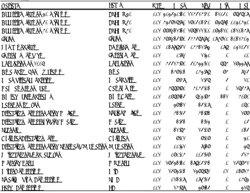
Figure 1: Income and Employment con…guration of Bogota (1.1e+06,3.0e+06] (660960,1.1e+06] (594726,660960] (346878,594726] (270396,346878] [196821,270396] Bogota (2007) Income (21442,142052] (14252,21442] (10471.5,14252] (5872,10471.5] (3074,5872] [197,3074] Bogota (2007) Employment

Author calculations based on data from Planning Department (Secretaria de planeacion del Distrito)

Figure 1 shows a disproportionate con…guration of employment and income in the city. It is easy to identify the axes where jobs and income are concentrated19_.

Two di¤erent “job centres” are connected on the same two axes. The city’s highest incomes are concentrated in two zones. These can be distinguished and they are also reliable on the same axis than the two jobs centres. This axis has the particularity that it bene…ts from the presence of TM. A third job axis is also placed alongside another Transmilenio axis. Regarding the other zones with high levels of income, they are not very far from the TM corridor that goes from the centre to the west of the city.

Additionally, jobs are condensed far from the boundaries of the city (with the exception of the East border). Even if we see that job centres are placed at the centre-east border of the city, this border was always considered as the “centre”. Executive and almost the 100% of administrative buildings are place on that zone. Furthermore, is in that place where Bogota was founded and it could not be expanded to the East because of the presence of a big chain of mountains

(Los Cerros Orientales). The expansion of the city took place essentially to the south and the north of the city and more recently to the west of the city.

Following the results of a poll made by the administration in 2005, most work travel moves from the "far" north, the south and the west to these four job centres. These are the zones with the lowest income in the city, with the exception of one zone in the north, where people with high purchasing power settled a few years ago, seeking to be far from the noise and pollution of the city. The “centre” of the city condensed more than 50% of jobs in the city and according to the poll, most of the people commuting to this zone of the city come from the north of the city. Others travel from the north-west, the west and the south and south-west of the city.

Apparently, this con…guration of Bogotanians’ jobs and income of can be directly related to the enhancement of the public transport system.

The next section will focus on analysis of this possible strong relationship. Results of the models proposed in section 2 will provide some elements support-ing knowledge of the existence and magnitude of this relation.

4

RESULTS AND DISCUTION

As stated above, analysis of the correlation matrix and the variance in‡ation factor (VIF) of all models is recommended.

The correlation matrix20 _{shows important relationships between some}

vari-ables21_{, in particular the variables “Population” and “Schools”. In e¤ect, the}

population has correlations above 0.50, with almost all the variables represent-ing the characteristics or the amenities of each zone. These correlations can be interpreted as reasonable. In e¤ect, the higher the population is, the more zones will need schools, parks, recreational facilities and sporting establishments. Likewise, if the population is bigger, it can be expected that the number of neigh-bourhoods will be greater as equal as the area of the zone. In despite of this, correlations just represent some control variables and not make part of the core of our analysis, it let infer that these correlations will not a¤ect the estimations. Nevertheless, the greater correlation is between the number of schools in zones and the number of establishments promoting sport and recreation (0.81). This is predictable if we consider that the most of the schools in Bogotá are public. They usually use the infrastructure of the zones (parks, and recreation establishments) for students’recreation and sporting activities.

2 0_{Annex 1.}

Another important correlation that relates to the goal of this study is between employment and improvement of public transport (number of stations); they have a correlation index equal to 0.56. It can be also awaited but it seems not to be a problem of multicollinearity if we consider that VIF is smaller than 10. It could also represent an additional argument to suggest that transport improvements directly a¤ect the number of jobs (model 3).

Other correlation indices above 0.50 are found. The big indices are principally between amenities variables, which is not very surprising and will not be a source of evils. None of those variables explain each other.

On the other hand, and as indicated previously for some relations between variables, regarding (VIF), no problems have been detected in the models22_{. On}

every model it is found that VIF < 10, which means that multicollinearity is low and dependent variables are uncorrelated with predictor variables.

The following section will present the results of OLS estimations and 2SLS estimations.

4.1

OLS Results

As noted previously, for the …rst stage of the analysis, each model – depending on the e¤ective size of the labour market –is regressed three times, in accordance with the three intervals of times. Table 2 shows results for the three models. There are three di¤erent results for models 1 and 2 and one result for model three.

4.1.1 Model 1: E¤ective Size of Labor Market

Regarding model 1, results show a not negligible R2 _{for each travel time, which}

goes from 0.583 when travel time is 40 minutes to 0.615 when travel time is 60 minutes. Taking into account the analysis of the correlation matrix and also the analysis of the VIF, it can be said that the model explains in an acceptable proportion the dependent variable.

Regarding regressors, table 2 suggests that improvement has a positive and big e¤ect on the level of the e¤ective size of labour market. In e¤ect, for a time period of 40 minutes, the number of Transmilenio stations seems to boost the size of the labour market of inhabitants of zone i on 15,200 jobs. Furthermore, for time intervals of 50 and 60 minutes, the presence of Transmilenio improvements in the zone has a positive relationship with the size of the labour market in the

order of 20,314 and 21,388 jobs respectively. These three results are signi…cant at the 0.05 level, which is not negligible.

Regarding income on each zone, it is also shown that it has a positive impact on the size of the labour market, which was predictable. The higher the income is, the higher will be the size of the labour market, because inhabitants may choose to live in a neighbourhood that is closer to their workplace. Nonetheless, in model 1, income seems not to have a signi…cant impact on ESLM .

Another variable that appears to signi…cantly impact the ESLM is the mean distance between inhabitants’homes and their jobs. This variable has a negative impact on the number of jobs reachable within these intervals of time. For the three di¤erent time periods, estimators of mean distance between reachable jobs and houses are signi…cant at the 0.01 level.

Additionally, its in‡uence on the level of ESLM looks to be very important. Actually, an additional kilometre of mean distance reduces the ESLM by 5% and 10% for any interval of time. It may seem strange but it can be considered normal. In e¤ect, concerning the ESLM , results con…rm the fact that, when individuals live far from their jobs, the number of reachable jobs relevant to their skills in the zone where they live may decrease. This means that the size of the labour market for people decreases if their jobs are far from their houses.

The variable Area is another variable that seems to be signi…cant from a statistical point of view. In e¤ect, table 2 shows that for any interval of time, it is signi…cant at a 0.05 level. Nevertheless it has always, a negative sign which can be estranged. Actually, regarding the area of the zone and its negative relationship with the size of the labour market for each population living in each zone, we can suggest that it could be because jobs and income are concentrated, in a big proportion, on small zones which are placed close to the job centres, while the biggest zones are placed at the periphery of the city.

People living in the biggest zones are those with smaller levels of income and are farther from job centres. In parallel, the bigger the area of each zone, the higher the number of neighbourhoods will be; that may also be the reason for the negative sign of the neighbourhoods parameter.

Table 2: OLS results for each interval of time

slm 40 slm 50 slm 60 income 40 income 50 income 60

711,644.313*** 1045928.176*** 1313650.550*** -136,230.614 -134,996.960 -209,878.949 -3,632.736 (79,704.801) (97,313.955) (97,115.364) (312,658.436) (344,254.457) (394,996.977) (5,667.080) 15,220.654** 20,314.682** 21,388.184** 25,161.388 26,034.941 25,842.513 3,274.915*** (7,523.774) (9,185.999) (9,167.252) (22,197.682) (22,362.994) (22,434.205) (534.947) 0.450 0.307 0.301 (0.292) (0.241) (0.242) 0.053 0.054 0.052 0.010*** (0.034) (0.042) (0.042) (0.002) -0.362 -0.324 -0.441 -3.854* -3.949* -3.918* -0.037 (0.723) (0.883) (0.881) (2.069) (2.074) (2.077) (0.051) -262.545** -385.040** -388.453** 336.586 338.087 337.181 21.047** (121.573) (148.432) (148.130) (360.452) (365.529) (365.922) (8.644) -35,218.349*** -45,881.804*** -50,838.129*** 6,305.226 4,437.753 5,676.773 -408.308 (7,161.193) (8,743.313) (8,725.470) (23,276.488) (23,691.774) (24,299.335) (509.167) -3.859 -1.873 -0.770 8.649 7.539 7.201 0.229 (3.465) (4.231) (4.222) (10.107) (10.101) (10.099) (0.246) 59.329** 75.797** 86.296*** 230.366*** 235.832*** 233.249*** 0.221 (26.480) (32.331) (32.265) (75.460) (75.799) (76.579) (1.883) -322.012 -781.846 -151.965 4,351.384** 4,478.577** 4,287.399** -89.009* (713.883) (871.601) (869.823) (2,031.430) (2,043.390) (2,039.829) (50.758) -933.344** -1,140.505** -1,007.571** -2,465.939** -2,558.896** -2,607.019** -7.563 (385.331) (470.462) (469.502) (1,126.882) (1,129.365) (1,121.241) (27.397) -2,964.688 -3,710.037 -2,941.590 -18,035.172 -18,382.453 -18,646.856 234.778 (5,759.372) (7,031.788) (7,017.438) (16,677.106) (16,739.421) (16,733.046) (409.496) 1,053.693 1,486.035 1,243.575 -4,910.330 -4,925.664 -4,847.548 -32.605 (1,644.851) (2,008.247) (2,004.149) (4,769.123) (4,790.947) (4,789.328) (116.950) -1,027.805 85.714 -1,576.168 17,458.404* 17,100.412* 17,612.816* 984.440*** (3,163.854) (3,862.843) (3,854.960) (9,036.689) (9,074.786) (9,075.872) (224.953) 5,871.716* 5,689.958 5,259.589 15,048.130 16,084.718* 16,256.850* 16.487 (3,270.352) (3,992.870) (3,984.722) (9,549.043) (9,510.627) (9,496.559) (232.525) -649.501 -765.556 -1,110.307* 638.618 583.495 683.448 -51.926 (516.125) (630.153) (628.867) (1,512.266) (1,517.503) (1,530.195) (36.697) Obs 112 112,00 112 112 112 112 112 R² 0.583 0.598 0.615 0.436 0.432 0.432 0.609 SLM Income _Employment Job_Accessibility Health Area Schools Cultural Recreation Neighborhoods Mean_dist Car owners Aver Cost Parks Social Welfare Intercept Improvment Income Population Author calculations

The estimator for the variable Average cost, which represents the average cost of travel that people have to pay to reach their job, appears with a positive sign on table 2. Moreover, this estimator is signi…cant at a 0.05 level with any travel time. It suggests that the more I pay for transport to reach my job, the higher will be the size of my labour market. It could also be expected if we consider that the price to be paid for use of the public transport we consider in this study (Transmilenio) is higher with respect to the other kind of public transport services, excepting taxis. Additionally, all Transmilenio lines were constructed on an axis passing by job centres, which makes Transmilenio the more expensive but, at the same time, the quicker transport system to reach job centres.

Regarding amenities in the zones, table 2 shows that four variables seem to have a negative e¤ect on the ESLM and two variables have positive impacts. Among these six amenities, just one has a signi…cant in‡uence on the dependent variable. SocialW elf are has, for the three intervals of time, a negative in‡uence on dependent variable with a signi…cance level of 0.05. It may be because this variable denotes the number of establishments like nursing homes, rehabilitation centres, orphanages and establishments promoting the welfare of inhabitants

with some problems interacting with society. In that vein, this kind of establish-ment may not have a positive e¤ect on the labour market because it requires a lot of space in the zone and employs fewer people than companies carrying out other activities. As with SocialW elf are, estimators of variables P arks and es-tablishments promoting cultural activities, Cultural, have a negative incidence on the ESLM but do not have signi…cant in‡uence on the dependent variable. Reasons may be the same as for SocialW elf are. P arks and Cultural take a lot of vital space in the zone and avoid the construction of roads, lines of transport systems and job centres.

Regarding establishments providing health services, Health, results show that they has a negative impact on ESLM . This seems to be counterintuitive because hospitals and health centres are supposed to create jobs. It suggests that the decision to construct hospitals in the city depends on the available area in each zone. In e¤ect, zones where job centres are situated do not have as many areas available for construction of hospitals as the peripheral zones do. In addition, the expensiveness of domiciliary public services on jobs centres could also in‡uence this relationship.

In summary, if a comparison of estimators of all variables is made, it can be said that the variable that most in‡uences ESLM is Improvement. In ad-dition, its in‡uence increases with respect to the commuting time, meaning the greater individuals’commuting time, the greater will be the in‡uence of public transports improvement on the e¤ective size of the labour market.

In opposition, the other variable that has a signi…cant but negative impact on the ESLM , with a statistical signi…cance of 0.01, is the mean distance that people have to commute to their jobs. As with improvement, M ean_dist in-creases with commuting time, which is expected. The higher the mean distance commuted by people, the lower the ESLM of inhabitants living on origin zones.

4.1.2 Model 2: Level of Income

Results for model 2 are also divided into three because one of the regressors is ESLM and it varies with respect to commuting time. On the other hand, while in‡uences of some estimators are not di¤erent from model 1, there are also …ve big di¤erences that have to be remarked upon.

First of all, the variable Improvement has a big in‡uence on the level of income of inhabitants of each zone. This suggests that the higher the presence of public transport improvements, the greater will be inhabitants’income. This relationship can be interpreted from two di¤erent points of view. In e¤ect, it is not false to suggest that the presence of Transmilenio can boost the income of inhabitants. On the other hand, it can also be said that people with greater levels of income choose to live in zones where there is more improvement of

urban transport. Nevertheless, it is clear that the impact of improvement of urban transport on the level of inhabitants’income cannot be denied. However, while the improvement estimator is the one that has the largest in‡uence on the level of income, it also has a problem in the OLS results: it is not statistically signi…cant. It represents another additional reason to carry out the 2SLS analysis in section 4.2.

The other di¤erence between model 1 and model 2 is that the estimators for Area, M ean_Dist, P arks, Cultural and N eighbourhoods are not negative but positive. First of all, regarding the area of the zone, it indicates that the bigger the zone, the greater the average income. This relationship is expected. In e¤ect, as suggested by Anas (1990), Glaeser, Kahn and Rappaport (2000) and other researchers, rich people sometimes prefer to live in suburbs or on zones far from the city to avoid the noise and the congestion of job centres. Additionally, in suburbs or zones far from the centre, rich people …nd more space to live or to construct bigger houses than those that they …nd downtown or near job centres. In parallel, amenities they prioritize, aside from housing space, are safety, calm (no noise or pollution), large green spaces to do sport and for their children to play in and proximity to nature, in spite of the need to consider proximity to their jobs or to the centre of the city. This is the reason for the large and positive in‡uences of estimators for P arks, Recreation, Cultural and N eighbourhoods, of which P arks and Cultural are those that are statistically signi…cant, at 0.05 and 0.1 respectively.

Regarding the Cultural estimator and establishments promoting cultural ac-tivities, it could be interpreted that cultural manifestations like theatre, opera and concerts, among others, are not a¤ordable for people with a limited income. Those kind of cultural expressions are revealed to be expensive, preventing ac-cessibility by people with a limited budget; that could be the reason for the positive and statistical signi…cance of this estimator on income.

In contrast, SocialW elf are, Health and Schools have a negative and not negligible in‡uence on the level of income, but only SocialW elf are is statisti-cally signi…cant (0.05). It can be interpreted as meaning that if there are more hospitals, schools, rehabilitation centres or nursing homes, this may lead to con-gestion; the calm of the zone can be a¤ected and people with bigger incomes may not be incentivized to live near those kinds of establishments. The easiest and best solution for people with high incomes is to live in distant and expensive suburbs with small density and with fewer establishments promoting health, so-cial welfare or schools. In opposition, people with low incomes also decide to live far from the city and job centres, but in suburbs or zones with high density and important concentrations of hospitals, schools and establishments providing social welfare. Likewise those variables, the negative and statistically signi…cant (0.01) impact of the variable P opulation is explained.

Finally, the other variable that reveals a statistically signi…cant impact on the level of income is Aver_Cost; this is also expected because if rich people

decide to live far from their jobs, they will be pushed (voluntarily) to expend more money to commute from their houses to their jobs.

As in model 1, model 2 reveals that the variable with more in‡uence on the dependent variable is the level of improvement of public transport in each zone. Nevertheless, with respect to the level of income, this variable is not signi…cant from a statistical point of view, and this leads us to the 2SLS analysis in section 2.2.

4.1.3 Model 3: Number of jobs

Model 3 shows the in‡uence of some explanatory variables on the number of jobs in each zone of the city. This model is measured with respect to the same independent variables as in model 1, but there is just one result because it does not depend on ESLM . Subsequently, even if the results are similar, there are also some important di¤erences that should be clari…ed.

The …rst di¤erence is that income is now statistically signi…cant, at 0.01, which was not the case in model 1. This may suggest that the number of jobs will be bigger in zones where income is higher, but it also may be proposed that enterprises or companies settle in zones or near zones where income is higher (Zenou, 2000, 2008; Ross, 1998; Kain, 1968).

Secondly, table 2 shows that the area of the zone has a positive and a sta-tistical signi…cance (0.05) to the number of jobs in each zone. The bigger the zone, the more jobs there will be in the zone. This result is the opposite from what was found in model 1, because model 1 tries to determine the impact of the area of the zone on the inhabitants’ number of reachable jobs. What was suggested in model 1 was that area has a negative impact on ESLM ; this is very di¤erent if the dependent variable is the number of jobs in each zone. ESLM takes into account reachable jobs for each inhabitant with respect to their skills and employment refers to all kinds of jobs in each zone. So, this could be the reason for this di¤ering relationship between models.

Another regressor that is signi…cant from a statistical point of view is the number of parks in each zone. This variable has a negative in‡uence on the number of jobs in each zone, which is logical because the more parks in each zone, the less available space there will be for the settlement of enterprises in the zone will be.

Fourthly, establishments promoting cultural activities seem to boost – and to create a signi…cant amount of –the number of jobs in each zone. This result suggests that cultural activities are an important source of employment for the city, equal to establishments providing health care. Schools seems to have the opposite e¤ect to Health or Cultural.

Aside all other results which are similar and could be read like those in model 1, the most important to note is that the variable with the bigger impact on the number of jobs on each zone is, once again, the number of Transmilenio stations. In addition to this, the estimator of this variable is signi…cant at 0.01 level, which demonstrates the great dependence of employment on improvements to public transport. It could signify that the number of employment grows by 3.274 if an additional Transmilenio station is built in a speci…c zone. However, it could also denote that enterprises decide to settle in zones with high levels of improvement to public transports and great levels of accessibility (Fernandez, 2008; Kawabata, 2003).

On the three precedent models, table 2 shows that the variable improvement has always a big and almost the greater in‡uence on the dependent variable, regardless of commuting time, when the variable ESLM is part of the model. Nonetheless, regarding the statistical signi…cance, this variable is not signi…cant in model 2.

2SLS analysis is then necessary to verify if the results of these models are not forgetting instruments that can determine or in‡uence the number of Trans-milenio stations on each zone. In other words, 2SLS analysis will let us verify if there exists an endogenous relationship between dependent variables of the three models and the variable improvement and, therefore, a causal relation between the number of stations in each zone and the dependent variables of each model.

4.2

2SLS Results

As de…ned in section 2.2, the third stage of this analysis is focused on the iden-ti…cation of endogeneity between the level of public transport and dependent variables. As for OLS results, it is essential to clarify that models 1 and 2 have three results depending on the commuting time.

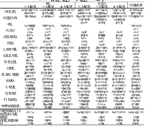
Additionally, the three models will also be regressed three times according to the de…nition of the Instrument Variable (IV ). In e¤ect, it is suggested that the decision to construct a Transmilenio station in a zone depends directly on the density, the workforce and the number of enterprises on each zone23_{. In}

that vein, the size or the number of employees of enterprises based in each zone should be taken into account and should be di¤erentiated. For that reason, this study proposed three di¤erent regressions of each model regarding the de…nition of the IV and in accordance with the size of companies established in each zone.

2 3_{See section 2.2 for de…nition of what it was called Microenterprises, Middle size enterprises} and Large enterprises

4.2.1 Enhancements of PT de…ned by the number of microenter-prises on zone i.

Results presented in this subsection correspond to models 1, 2 and 3 when the VI is de…ned by the density, the workforce in each zone and the number of microenterprises in each zone.

First of all, table 3 shows that every estimator has the same relationship (sign) and the same statistical signi…cance for model 1 than on OLS results. Im-provement is the variable that has the higher positive and statistical in‡uence on the size of the labour market in each zone. In parallel, the mean distance be-tween houses and jobs is the variable that has the higher negative and statistical impact on the dependent variable.

Table 3: 2SLS results for each interval of time when: impro = ₀+ 1W Fi+ 2M iEsi

40 minutes 50 minutes 60 minutes 40 minutes 50 minutes 60 minutes

703,963.433*** 1031718.345*** 1302852.910*** -121,333.320 -108,458.695 -159,857.237 -10,059.739 (76,209.254) (93,583.480) (93,355.711) (314,339.274) (323,163.063) (372,672.907) (6,948.676) 22,117.543* 32,521.548** 31,071.155** 40,792.818 41,285.053 43,053.538 7,588.386*** (12,173.235) (14,948.495) (14,912.112) (38,949.393) (36,786.388) (36,908.604) (1,109.942) 0.394 0.258 0.243 (0.306) (0.236) (0.238) 0.047 0.043 0.044 0.007** (0.033) (0.041) (0.040) (0.003) -0.441 -0.423 -0.578 -3.634* -3.729* -3.694* -0.012 (0.671) (0.824) (0.822) (2.060) (1.922) (1.925) (0.061) -0.020** -0.029** -0.028** 0.025 0.024 0.024 0.002** (0.010) (0.012) (0.012) (0.031) (0.029) (0.029) (0.001) -36,208.470*** -47,168.293*** -52,548.061*** 6,706.096 4,535.453 5,150.545 -177.267 (6,614.546) (8,122.534) (8,102.765) (23,290.065) (22,132.616) (22,823.788) (603.107) -3.272 -0.892 0.086 9.093 8.080 7.885 0.484 (3.307) (4.061) (4.052) (10.239) (9.555) (9.574) (0.302) 59.490** 76.436** 86.289*** 236.064*** 241.762*** 240.669*** 0.977 (24.888) (30.562) (30.487) (75.742) (70.807) (71.623) (2.269) -324.728 -774.181 -159.629 4,440.929** 4,544.679** 4,388.467** -62.548 (671.884) (825.060) (823.052) (2,038.148) (1,907.578) (1,905.703) (61.262) -905.372** -1,094.140** -966.178** -2,472.263** -2,569.331** -2,614.283** 4.153 (362.732) (445.428) (444.344) (1,130.620) (1,053.969) (1,047.196) (33.074) -3,834.870 -5,175.738 -4,215.141 -19,269.376 -19,584.524 -19,986.315 -174.459 (5,490.552) (6,742.291) (6,725.881) (17,005.259) (15,888.868) (15,885.761) (500.622) 763.630 979.882 839.208 -5,357.926 -5,340.447 -5,325.691 -191.838 (1,588.269) (1,950.364) (1,945.617) (4,889.940) (4,567.202) (4,571.254) (144.817) -353.538 1,227.071 -595.260 18,263.733* 17,930.487** 18,462.362** 1,309.516*** (3,065.944) (3,764.920) (3,755.757) (9,293.874) (8,707.936) (8,684.017) (279.549) 5,340.337* 4,722.659 4,513.505 13,805.633 14,835.026 14,872.610 -385.920 (3,202.302) (3,932.365) (3,922.794) (9,940.897) (9,245.787) (9,239.208) (291.982) -699.074 -834.504 -1,196.246** 660.919 603.795 677.960 -52.580 (482.502) (592.503) (591.061) (1,516.013) (1,415.777) (1,432.348) (43.994) Endogeneity Wu -Hausman F Test 0.44933 0.94049 0.58849 0.22424 0.20373 0.25837 48.18274*** Sargan 3.337 4.646* 1.956 4.002 4.158 4.459 2.690 Heterocedasticity 19.211 18.153 15.928 36.676 *** 36.388 *** 34.986 *** 19.623 R² 0.576 0.586 0.605 0.432 0.428 0.427 0.346

Standard errors in parentheses *** p<0.01, ** p<0.05, * p<0.1 Neighborhoods Parks Social Welfare Health Schools Cultural Recreation Aver Cost SLM Income _Employment Intercept Improvment SLM Income Population Area Mean_dist Car owners Author calculations

Although there is a similarity between OLS and 2SLS results for model 1, the impact of the number of stations on the size of the labour market is 50% higher with respect to OLS model results. .Following this observation, it is suggested that when improvement is treated as an IV depending on the number of microenterprises, its impact on the dependent variable increases by 50%.

Regarding the endogeneity analysis, table 3 reveals that even if the number of stations in each zone remains signi…cant and greater than in OLS regressions, and even if there is no problem regarding the choice of instruments that explain IV , the variable improvement is not endogenous to the size of the labour market. This result is counterintuitive to the objective that this investigation tries to demonstrate but one fact is salvageable, which is that when improvement is considered as a IV , its statistical signi…cance and its impact on ESLM increase by 50%.

Concerning model 2, 2SLS results are not signi…cantly di¤erent from those found in OLS estimations. Similarly, relationships between variables are re-spected and every estimator preserves the same sign, the same statistical signif-icance and almost the same level. It means that the number of stations in each zone is not yet statistically signi…cant but their e¤ect on ESLM is almost 70% higher than in the OLS models.

As in the previous model, selected instruments do not have problems of over-identi…cation but the analysis of endogeneity displays that “improvement”is not endogenous to the income of each zone’s inhabitants. It was not what the study had expected and it will be explained at the end of all 2SLS results’discussion.

Results for model 3 are slightly di¤erent. Variables such as income, P opulation, Aver_Cost and Car_owners preserve the same impact and the same statisti-cal inference on the dependent variable as in OLS results. Likewise, the mean distance between homes and jobs has the same relationship as in the OLS model but its in‡uence on independent variable increases by 100%. In addition, even if the variable Area has the same statistical in‡uence (0.05) on the number of jobs as in the OLS model, its “real” impact is marginally (0.002) contrary to the number of parks on each zone that is no longer statistical signi…cant but its real in‡uence on employment is also negligible. The other group of variables does not have a signi…cant in‡uence on the number of jobs in each zone, with the exception of two variables that are very signi…cant and that have a notable in‡uence on the number of jobs.

The two regressors that have a signi…cant e¤ect on employment in each zone are the number of establishments promoting cultural activities and the number of stations in each zone. Regarding Cultural, its statistical signi…cance is high (0.01). This result could signify that the implantation of one additional estab-lishment promoting cultural activities could raise by 1.309 the number of jobs in each zone. On the other hand, this result could be interpreted di¤erently; the target population of that kind of establishment could be employees, but this study does not have more enough information to make this statement.

With respect to the number of stations, as in the OLS results, it can be ob-served that this is the regressor with the greater e¤ect on the explained variable. When improvement is considered as endogenous and when it depends on the number of microenterprises, its in‡uence on the number of jobs in each zone is double that of the OLS model. In addition, its statistical signi…cance is still very high (0.01). In e¤ect, an additional station in each zone is supposed to boost the number of jobs by 7,560. Besides, it can also be supposed that Transmilenio stations were built with the aim to be close to employment centres. Neither hypothesis moves away from the goal of this analysis, which is to demonstrate the causal relation between the number of jobs in each zone and the level of improvement to public transports.

Regarding this statement, endogeneity test reveals that improvement is en-dogenous to the number of jobs on each zone. In other words, the number of Transmilenio stations is endogenous with respect to the number of jobs. This result implies that the hypothesis is veri…ed, which enables us to prove the fol-lowing hypothesis:

H0: (improvement) = 0(exogeneity)

H1: (improvement) = 0(endogeneity)

The p-value of Wu-Hausman F test is statistically signi…cant (0.01), which leads to rejecting the null hypothesis of exogeneity, H0. The endogeneity in the

relation between improvement and the number of jobs in each zone is demon-strated.

This result is even truer if, the test of over-identifying restrictions, “Sargan N*R-sq test”24_{, and heterocesdasticity test (Pagan-Hall}25_{) are taken into}

con-sideration. In fact, those tests demonstrate that instruments have no problems of over-identi…cation and heteroscedasticity (no rejection of null hypothesis). This means that instruments are exogenous and the residuals of the main model are uncorrelated with the set of instrumental variables. Instruments were well chosen.

Considering results for models 1 and 2, OLS results appear to be consistent. In e¤ect, improvement is not endogenous when it is regressed depending on density, working force and microenterprises. By contrast, OLS results are not consistent for model 3. In fact, suspicions of endogeneity of improvement are corroborated, which represents an undeniable causality relation from enhance-ment of urban transport to the number of jobs when the number of stations are de…ned by microenterprises.

2 4_{The joint null hypothesis is that the instruments are valid instruments, i.e., uncorrelated} with the error term, and that the excluded instruments are correctly excluded from the esti-mated equation. Under the null, the test statistic is distributed as chi-squared in the number of (L-K) overidentifying restrictions. A rejection casts doubt on the validity of the instruments.

2 5_H

4.2.2 Improvement regressed with respect to “small and middle size” enterprises

Results presented in this subsection correspond to models 1, 2 and 3 where the variable suspected to be endogenous is de…ned by the density, the work force in each zone and the number of middle-size enterprises in each zone.

Results for model 1 express exactly the same relationships as in the previous subsection. This means that there is no evidence to reject the use of instru-mental variables on the model. In e¤ect, Sargan test shows that there is no over-identi…cation of instrumental variables likewise with the heteroscedasticity test that con…rm that the variables are homoscedastic. Nevertheless, as in the previous model, Endogeneity – Wu-Hausman F test allows to accept null hy-pothesis of exogeneity; the number of stations on each zone of the city are not endogenous on the e¤ective size of labour market. Taking into account those previous observations, it can be con…rmed that OLS results are consistent for model 1.

In contrast, the results for model 2 suppose di¤erent interpretations. The variable P opulation continues to have the same impact on the dependent vari-able but it ceases to have statistical signi…cance; also, Social_W elf are preserves its in‡uence on Income but is no longer signi…cant at 0.05; rather it is at 0.1. On the other hand, establishments providing health services increase their negative in‡uence on the level of income by 70% more than when improvement is de…ned by SM E. Additionally, this variable has a statistical signi…cance of 0.1, which is not very representative but suggests that if the number of middle-size enter-prises is taken into account at the moment to de…ne the variable improvement, an additional establishment providing health in the zone will lower the income of inhabitants by 34.500 COP26. It represents a decrease of 8%27 of the minimum wage established by the government on 2007. These results could suggest that inhabitants with higher incomes prefer to live in zones with few promoters enti-ties of health. The income of inhabitants living in zones with several promoter entities of health is 34.500 COP lower than that of inhabitants of zones with few of those kinds of establishments, which represents 8% of minimum wage for that year.

Regarding the number of Transmilenio stations in a zone and their e¤ect on the level of income, table 4 reveals that this in‡uence is notable. In e¤ect, results suggest that one additional Transmilenio station will boost the income of inhabitants by 197.000 COP28_{, which represents 28% of the average wage of}

a citizen and 45% of the minimum wage decreed by the Colombian government

2 6_{COP: Colombian Pesos. The exchange rate on 2007 was: 1 USD = 2078 COP; 34.500} COP = 16.6 USD

2 7_{The minimum wage represents the minimum wage that a worker have to be paid monthly;} on 2007, the minimum wage in Colombia was 433.700 COP = 208 USD.