Using satellite data to improve the leaf phenology of a global terrestrial biosphere model

HAL Id: hal-01805153

https://hal.archives-ouvertes.fr/hal-01805153

Submitted on 27 Oct 2020

HAL is a multi-disciplinary open access

archive for the deposit and dissemination of

sci-entific research documents, whether they are

pub-lished or not. The documents may come from

teaching and research institutions in France or

abroad, or from public or private research centers.

L’archive ouverte pluridisciplinaire HAL, est

destinée au dépôt et à la diffusion de documents

scientifiques de niveau recherche, publiés ou non,

émanant des établissements d’enseignement et de

recherche français ou étrangers, des laboratoires

publics ou privés.

global terrestrial biosphere model

N. Macbean, F. Maignan, P. Peylin, C. Bacour, Francois-Marie Breon, P. Ciais

To cite this version:

N. Macbean, F. Maignan, P. Peylin, C. Bacour, Francois-Marie Breon, et al.. Using satellite data

to improve the leaf phenology of a global terrestrial biosphere model. Biogeosciences, European

Geosciences Union, 2015, 12 (23), pp.7185 - 7208. �10.5194/bg-12-7185-2015�. �hal-01805153�

www.biogeosciences.net/12/7185/2015/ doi:10.5194/bg-12-7185-2015

© Author(s) 2015. CC Attribution 3.0 License.

Using satellite data to improve the leaf phenology of a global

terrestrial biosphere model

N. MacBean1, F. Maignan1, P. Peylin1, C. Bacour2, F.-M. Bréon1, and P. Ciais1

1_{Laboratoire des Sciences du Climat et de l’Environnement, Gif sur Yvette CEDEX, 91191, France} 2_{NOVELTIS, Labège, 31670, France}

Correspondence to: N. MacBean (nlmacbean@gmail.com)

Received: 24 July 2015 – Published in Biogeosciences Discuss.: 19 August 2015

Revised: 16 November 2015 – Accepted: 22 November 2015 – Published: 10 December 2015

Abstract. Correct representation of seasonal leaf

dynam-ics is crucial for terrestrial biosphere models (TBMs), but many such models cannot accurately reproduce observa-tions of leaf onset and senescence. Here we optimised the phenology-related parameters of the ORCHIDEE TBM us-ing satellite-derived Normalized Difference Vegetation In-dex data (MODIS NDVI v5) that are linearly related to the model fAPAR. We found the misfit between the observa-tions and the model decreased after optimisation for all bo-real and temperate deciduous plant functional types, primar-ily due to an earlier onset of leaf senescence. The model bias was only partially reduced for tropical deciduous trees and no improvement was seen for natural C4 grasses. Spa-tial validation demonstrated the generality of the posterior parameters for use in global simulations, with an increase in global median correlation of 0.56 to 0.67. The simulated global mean annual gross primary productivity (GPP) de-creased by ∼ 10 PgC yr−1 over the 1990–2010 period due to the substantially shortened growing season length (GSL – by up to 30 days in the Northern Hemisphere), thus reduc-ing the positive bias and improvreduc-ing the seasonal dynamics of ORCHIDEE compared to independent data-based estimates. Finally, the optimisations led to changes in the strength and location of the trends in the simulated vegetation productivity as represented by the GSL and mean annual fraction of ab-sorbed photosynthetically active radiation (fAPAR), suggest-ing care should be taken when ussuggest-ing un-calibrated models in attribution studies. We suggest that the framework presented here can be applied for improving the phenology of all global TBMs.

1 Introduction

Leaf phenology, the timing of leaf onset, growth and senes-cence, is a critical component of the coupled soil–vegetation– atmosphere system as it directly controls the seasonal ex-changes of carbon, C, as well as affecting the surface en-ergy balance and hydrology through changing albedo, sur-face roughness, soil moisture and evapotranspiration. In turn leaf phenology is largely governed by the climate, as leaf onset and senescence are triggered by seasonal changes in temperature, moisture and radiation. Leaf phenology is there-fore sensitive to inter-annual climate variability and future climate change (Cleland et al., 2007; Körner and Basler, 2010; Reyer et al., 2013), as well as to increasing atmo-spheric CO2 concentrations (Reyes-Fox et al., 2014), and

will provide feedback on both climate and atmospheric C02 (Richardson et al., 2013). It is expected that climate warm-ing will advance leaf onset in temperature limited north-ern biomes. Such trends have already been observed in the Northern Hemisphere (NH) using either satellite or in situ observations (Badeck et al., 2004; Delbart et al., 2008; Jeong et al., 2011; Myneni et al., 1997; Parmesan, 2007). However, increasing temperatures may either advance or delay senes-cence, depending on species-specific responses to other envi-ronmental variables (Hänninen and Tanino, 2011; Piao et al., 2007). Future changes of precipitation in a warming climate will also likely affect tropical and semi-arid ecosystems that are more controlled by moisture availability (e.g. Anyamba and Tucker, 2005; Dardel et al., 2014; Fensholt et al., 2012). In order to improve predictions of the impact of future cli-mate change on vegetation and its interaction with the global C and water cycles, it is crucial to have prognostic leaf

phe-nology schemes in process-based terrestrial biosphere mod-els (TBMs) that constitute the land component of Earth sys-tem models (ESMs) (Kovalskyy and Henebry, 2012b; Levis and Bonan, 2004). Many such models exist in the literature, especially for temperate and boreal forests (e.g. Arora and Boer, 2005; Caldararu et al., 2014; Chuine, 2000; Hänninen and Kramer, 2007; Knorr et al., 2010; Kovalskyy and Hene-bry, 2012a) and have been included in most TBMs. However, model evaluation studies have shown that there are biases in the growing season length and magnitude of the leaf area in-dex (LAI) predicted by TBMs when compared to ground-based observations of leaf emergence and LAI (Kucharik et al., 2006; Richardson et al., 2012) or satellite-derived mea-sures of vegetation greenness and LAI (Kim and Wang, 2005; Lafont et al., 2012; Maignan et al., 2011; Murray-Tortarolo et al., 2013). This can result in systematic errors in model pre-dictions of the seasonal carbon, water and energy exchanges (Kucharik et al., 2006; Richardson et al., 2012; Walker et al., 2014).

As is always the case prior to model parameter calibra-tion, it is unclear whether the misfit between modelled and observed measures of leaf phenology is the result of inac-curate parameter values, model structural error, or both. In order to answer this question, the parameters first need to be optimised using data assimilation (DA) techniques, and if the models cannot reproduce the data within defined uncer-tainties we expect to gain insights into possible directions for model improvement. DA is also a useful way to better charac-terise and possibly reduce uncertainty in model simulations, and to determine the relative influence of parametric, struc-tural and driver uncertainty (e.g. Migliavacca et al., 2012).

Many studies have optimised the parameters of phenol-ogy models for a range of species with ground-based obser-vations of the date of leaf onset (Blümel and Chmielewski, 2012; Chuine et al., 1998; Fu et al., 2012; Jeong et al., 2012), the “green fraction” derived from ground-based digital pho-tography (Migliavacca et al., 2011) or with spring onset dates derived from carbon fluxes taken at flux tower sites (Melaas et al., 2013). Melaas et al. (2013) went further and demon-strated the transferability of parameters in time and between sites by including multiple sites in the optimisation. All of these studies have used DA to test different phenology model structures, thereby contributing significantly to the debate about whether a simple classical temperature-driven budburst model is sufficient, or whether more complex chilling and/or photoperiodic cues are needed to best predict leaf onset. Sev-eral studies also investigated the impacts of optimising phe-nology on the resulting C and water budgets (Migliavacca et al., 2012; Picard et al., 2005; Richardson and O’Keefe, 2009).

Peñuelas et al. (2009) noted that medium- to coarse-resolution satellite data might be more appropriate for op-timising the phenology in TBMs, due to the large differ-ence in scale between the resolution of a typical model grid cell (1 × 1◦) and ground-based data, which may cause

representation errors (Rayner, 2010). A few studies to date have performed a global optimisation of model phenology using satellite data, in the sense that multiple sites and/or plant functional types (PFTs) are included in the assimila-tion (Forkel et al., 2014; Knorr et al., 2010; Stöckli et al., 2011). In this study we aim to reinforce this line of research and to answer the following questions:

i. Can we constrain the phenology-related parameters and processes of a typical process-based TBM at global scale using satellite “greenness” index data?

ii. Does this produce a generic parameter set that results in improved simulations of the seasonal cycle of the vege-tation, or are further model structural developments re-quired?

iii. What is the impact of the optimisation on mean patterns and trends in vegetation productivity (as represented by the mean fraction of absorbed photosynthetically ac-tive radiation (fAPAR), amplitude and growing season length (GSL)) at regional and global scales?

To achieve this we performed a global, PFT, multi-site optimisation of the phenology model parameters for the six non-agricultural deciduous PFTs of the ORCHIDEE TBM. The phenology models in ORCHIDEE are common to many process-based TBMs. Note there is no specific phenol-ogy model associated to evergreen PFTs, where leaf turnover is simply a function of climate and leaf age.

Some of the carbon cycle-related parameters of OR-CHIDEE (including phenology-related parameters) have previously been optimised using in situ flux measurements (e.g. Kuppel et al., 2014; Santaren et al., 2014; Bacour et al., 2015). Here we focus purely on improving the timing of both spring onset and autumn senescence of ORCHIDEE at global scale, by using a novel approach to assimilate normalised medium-resolution satellite-derived vegetation “greenness” index data (MODIS NDVI collection 5) that are linearly re-lated to the simure-lated daily fAPAR. The aim of a multi-site (MS) (i.e. model grid cell) assimilation is to find a unique parameter set for each PFT that results in a similar improve-ment as a single-site (SS) optimisation, as the range of pos-terior parameter values for individual sites/species can be large (Richardson and O’Keefe, 2009). We hypothesise that the MS approach may average out the site-based variability, and thus provide one consistent PFT-generic parameter vec-tor that can be used for global simulations (e.g. Kuppel et al., 2014).

2 Methods and data

2.1 ORCHIDEE terrestrial biosphere model

ORCHIDEE is a global process-oriented TBM (Krinner et al., 2005) and is the land surface component of the IPSL-CM5 Earth System Model (Dufresne et al., 2013). In this

study we used the “AR5” version that was used for the IPCC Fifth Assessment Report (Ciais et al., 2013). The model cal-culates carbon, water and energy fluxes between the land sur-face and the atmosphere at a half-hourly time step. The water and energy module computes the major biophysical variables (albedo, roughness height, soil humidity) and solves the en-ergy and hydrological budgets. The carbon module controls the uptake of carbon into the system and respiration follow-ing cyclfollow-ing of C through the litter and soil pools. Carbon is assimilated via photosynthesis depending on light avail-ability, CO2 concentration and soil moisture, based on the

work of Farquhar et al. (1980) for C3 plants and Collatz et al. (1992) for C4 plants. The module includes the calcula-tion on a daily time step of a prognostic LAI and alloca-tion of newly formed photosynthates towards leaves, roots, sapwood, reproductive structures and carbohydrate reserves, depending on the availability of moisture, light availability and heat (Friedlingstein et al., 1999). The phenology mod-els that control the timing of leaf onset and senescence in ORCHIDEE, depending on PFT, were described in Botta et al. (2000) and Maignan et al. (2011) but are described in more detail in Appendix A. The simulated fAPAR can be calculated from the model LAI using the following Beer-Lambert extinction law, assuming a spherical leaf angle dis-tribution and that the sun is at nadir (following Bacour et al., 2015):

fAPAR = 1 − e−0.5LAI. (1)

ORCHIDEE’s functioning relies on the concept of plant functional types (see Wullschleger et al. (2014) for a review). A PFT groups plants that have the same physiological be-haviour under similar climatic conditions. ORCHIDEE uses 13 PFTs that are listed in Table 1 (along with the phenol-ogy model used). Different PFTs share the same processes but usually with different parameter values, except for the phenological models that are PFT-dependent (Table 1). The model is driven by meteorological variables related to tem-perature, precipitation, short- and long-wave incident radia-tion, specific humidity, surface pressure and wind speed. Soil texture and PFT fraction are also prescribed per grid cell.

2.2 Satellite data

2.2.1 Observing the seasonal cycle of vegetation

The seasonal cycle of the terrestrial vegetation is observed daily, cloud cover permitting, at a global scale and medium-scale spatial resolution (250 m) from several polar orbiting spectroradiometers. Studies have shown that considerable discrepancies exist between so-called “high-level” satellite products such as LAI or fAPAR, especially when consider-ing their magnitude (D’Odorico et al., 2014; Garrigues et al., 2008; Pickett-Heaps et al., 2014). This is because ra-diative transfer models are used to derive these products, which introduces uncertainty due to undetermined

parame-Table 1. Standard PFTs used in ORCHIDEE, their short name and

corresponding phenology model (see Appendix A for a full descrip-tion of the phenology models). Evergreen and agriculture PFTs do not have a specific phenology model in the ORCHIDEE TBM.

PFT Description Short name Phenology model

1 Bare soil BS –

2 Tropical broadleaved evergreen TrBE –

3 Tropical broadleaved raingreen TrBR MOI

4 Temperate needleleaf evergreen TeNE –

5 Temperate broadleaved evergreen TeBE –

6 Temperate broadleaved deciduous TeBD NCD_GDD

7 Boreal needleleaf evergreen BoNE –

8 Boreal broadleaved deciduous BoBD NCD_GDD

9 Boreal needleleaf deciduous BoND NGD

10 Natural C3 grass NC3 MOI_GDD

11 Natural C4 grass NC4 MOI_GDD

12 C3 crops (agriculture) AC3 –

13 C4 crops (agriculture) AC4 –

ters or potentially incomplete descriptions of the radiative transfer model physics. Instead therefore, we considered a vegetation greenness index, the Normalized Difference Veg-etation Index (NDVI), that is directly related to the near in-frared (NIR) and red (RED) surface reflectance, ρ (NDVI =

ρNIR − ρRED / ρ NIR +ρRED). This index is based on the fact that photosynthesising vegetation reflects a high propor-tion of the incoming NIR radiapropor-tion, whilst absorbing most of the red. NDVI has been shown to be linearly related to fAPAR, though with uncertainties related to the issues men-tioned above (Fensholt et al., 2004; Knyazikhin et al., 1998; Myneni and Williams, 1994). Therefore although NDVI is not directly related to a physical property of the vegetation, it does capture its seasonal cycle together with inter-annual anomalies, and therefore can be used to optimise the model phenology (via the simulated fAPAR). In order to optimise the seasonality (but not the magnitude) of modelled daily fA-PAR using the NDVI data, we normalise both to their max-imum and minmax-imum values of the whole time series at each site (following Bacour et al., 2015).

2.2.2 MODIS NDVI data and processing

NDVI observations are derived from the MOD09CMG col-lection 5 (v5) surface red (620–670 nm) and near-infrared (841–876 nm) daily global reflectance products available at 5 km from the MODerate resolution Imaging Spectrome-ter (MODIS) on-board the NASA’s Terra satellite. The re-flectance data were cloud-screened and corrected for atmo-spheric and directional effects (related to the change of re-flectance with observation geometry) following (Vermote et al., 2009), and the corresponding NDVI was calculated for the 2000–2008 period. The time series were interpolated on a daily basis, in order to account for any missing values due to cloud, using a third degree polynomial and considering the 10 nearest valid acquisitions, with a maximum allowed difference of 15 days. The NDVI values were then spatially

averaged at the model forcing spatial resolution (0.72◦_{) for} each time step. The data have a noise range of ∼ 0.025 to 0.03, with highest values in densely forested areas (Vermote et al., 2009). However, in this study the daily model and ob-servation uncertainty used in the assimilation was defined as the RMSE between the normalised prior model fAPAR simu-lation (using default ORCHIDEE values) and the normalised NDVI observations, following (Kuppel et al., 2012). This er-ror thus accounts for the spatial and temporal averaging, the error of the NDVI retrieval and the model structural error.

2.3 Data assimilation procedure

2.3.1 System description

The ORCHIDEE Data Assimilation System (http://orchidas. lsce.ipsl.fr) is based on a variational data assimilation pro-cedure that has been described in detail in previous studies using ground-based net surface CO2and energy fluxes

(Kup-pel et al., 2012; Santaren et al., 2007; Verbeeck et al., 2011). Kuppel et al. (2012) presented the first results using a multi-site (MS) version of the system at selected eddy-covariance flux tower locations, where data from all sites were used to optimise the model parameters at the same time for each PFT. As with most statistical data assimilation approaches it fol-lows a Bayesian framework, where prior knowledge of the parameter values is updated based on new information from the observations. Assuming that the probability distribution functions (PDFs) of the model parameter and observation un-certainties are Gaussian, the optimal parameter vector x can be found by minimising the following cost–function J (x) (Tarantola, 1987):

J (x) =1

2[(H (x) − y)R

−1_{(H (x) − y)}T

+(x − xb)P−_b1(x − xb)T], (2) where y is the observation vector, H (x) the model outputs, given parameter vector x, R the uncertainty matrix of the ob-servations (including observation and model errors), xbthe a priori parameter values (the standard values of ORCHIDEE) and Pb the a priori uncertainty matrix of the parameters. Hence, the cost function describes the misfit between the ob-servations and corresponding model outputs, plus the misfit between the current and prior parameter vectors, weighted by prior information on the parameter and observation un-certainties. Observation and model errors are assumed to be uncorrelated in space and time, and parameters are assumed to be independent; hence R and Pb are diagonal matrices. The cost function is iteratively minimised using the gradient-based L-BFGS-B algorithm (Byrd et al., 1995), which allows the definition of boundary constraints for the parameters. The prior parameter vector is most commonly used as the starting point in the iterative minimisation, but it can be started from any point (set of parameter values) in the parameter space. The gradient of the J (x) is estimated using the tangent

lin-ear model, except for parameters that impose a threshold on the model processes. For these, the finite difference method is used.

The posterior parameter covariance can be approximated from the inverse of the second derivative (Hessian) of the cost function around its minimum, which is calculated using the Jacobian of the TBM model with respect to fAPAR at the minimum of J (x) (for the set of optimised parameters), H∞, following Tarantola (1987):

Ppost= [HT∞R

−1_H

∞+P−_b1]−1. (3) The posterior parameter covariance can then be propa-gated into the model state variables (fAPAR or net C flux) space given the following matrix product and the hypothesis of local linearity (Tarantola, 1987):

Rpost=HPpostHT. (4)

The square root of the diagonal elements of Rpost

corre-sponds to the posterior error (standard deviation σ ), on the state variables considered of each grid cell. In order to ap-praise the knowledge improvement brought by the assimila-tion, the error reduction is determined as 1 − Rpost/Rprior).

2.3.2 Parameters to be optimised

Figure 1 shows a general schematic of how the parameters of the phenological equations used in ORCHIDEE (Botta et al., 2000) control the timing of the seasonal cycle of the LAI as well as the rate of leaf growth and fall. The pa-rameters that are optimised for each PFT are given in Ta-ble 2 and are briefly described here. A more detailed de-scription can be found in Appendix A. The start of the sea-sonal cycle of temperature-driven PFTs is constrained by optimising the growing degree day threshold, GDDthreshold

(Eqs. A1 and A2), the threshold for the number of growing days, NGDthreshold and the LAIthreshold(Eq. A4) parameters,

which all play a part in controlling leaf onset and rate of canopy growth. As the GDDthreshold is calculated in

differ-ent ways depending on the PFT-dependdiffer-ent phenology model used, and as the NGDthreshold acts in a similar way to the

GDD models, we introduced one single multiplicative effec-tive parameter, Kpheno_crit, to optimise the GDDthreshold and

NGDthresholdfor all phenology models. Thus the GDDthreshold

and the NGDthresholdbecome the following:

GDDthreshold=Kpheno_critGDDthreshold (5)

NGDthreshold=Kpheno_critNGDthreshold, (6)

with an a priori value of 1. In a similar manner a new ef-fective parameter, Klai_happywas introduced to compute the

LAIthresholdparameter, which is the LAI below which the

car-bohydrate reserves are used for leaf growth at the beginning of the growing season, following the equation

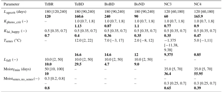
Table 2. ORCHIDEE parameters optimised. For each PFT the prior values, minimum and maximum values (in squared brackets) and

multi-site posterior mean values (in bold) are given. Note the prior uncertainty on the parameters is defined as 40 % of the full parameter range.

Parameter TrBR TeBD BoBD BoND NC3 NC4

Lagecrit(days) 180 [120,240] 180 [90,240] 180 [90,240] 180 [90,240] 120 [60,180] 120 [60,180] 120 160.6 240 90 60 165.9 K_{pheno_crit}(−) – 1.0 [0.7, 1.8] 1.0 [0.7, 1.8] 1.0 [0.7, 1.8] 1.0 [0.7, 1.8] 1.0 [0.7, 1.8] 1.13 0.87 1.1 0.77 0.9 Klai_happy(−) 0.5 [0.35, 0.7] 0.5 [0.35, 0.7] 0.5 [0.35, 0.7] 0.5 [0.35, 0.7] 0.5 [0.35, 0.7] 0.5 [0.35, 0.7] 0.7 0.4 0.36 0.35 0.35 0.47 Tsenes(◦C) – 12.0 [2, 22] 7.0 [−3, 17] 2.0 [−8, 12] −1.375 [−11.38, 9.38] 5.0 [−1,11] 16.6 14.6 12 9.375 0.85 Lfall(−) 10.0 [2, 50] 10.0 [2, 50] 10.0 [2, 50] 10.0 [2, 50] – – 10.0 29.5 4.7 9.0

Moist_Tmin(days) 50 [10, 100] – – – 35.0 [5, 70] 35.0 [5, 70]

10 36.4 55.95

Moistsenes, no_senes(−) 0.3 [0.2, 0.8] – – – – – – – – 0.3 [0.25, 0.7] – 0.3 [0.25, 0.7] 0.8 0.65 0.39

Critical leaf age!

Lagecrit!

Rate of leaf fall!

Lfall!

For grasses!

Temperature or moisture threshold for senescence! Tsenes and Moistno_senes! Fraction of carbohydrate reserve used for leaf growth! Klai_happy!

Scalar of temperature threshold and/ or time since moisture minimum!

Kpheno_crit and MoistTmin!

Figure 1. Schematic to show how the optimised parameters control

the timing of the leaf phenology in ORCHIDEE. The dotted arrow shows that the temperature and moisture threshold for senescence also affects the rate of leaf fall for grasses by slowing down the turnover rate once this threshold has been reached (whereas for trees only the Lfallparameter is used).

Although it is not strictly a phenology model parameter, we optimise Klai_happyas it is partly responsible for the rate of

leaf growth. LAImaxis a fixed parameter in this study as we

only examine the seasonal cycle of the vegetation, not its magnitude.

The end of the seasonal cycle is constrained by optimis-ing the critical leaf age for senescence, Lagecrit(Eq. A5), the

senescence temperature threshold, Tthreshold(Eq. A6) and the

rate of leaf fall, Lfall (Eq. A8) parameters. Lagecrit and Lfall

are optimised directly, and Tthresholdis optimised through the C0parameter (Eq. A6), and is henceforth called Tsenes.

For phenology models that are driven by soil moisture con-ditions (“MOI” models – see Appendix A and Table 1) the

parameter that controls leaf onset is the “minimum time since the last moisture minimum” (MoistTmin), and the parameters

that control senescence are Moistsenesand Moistno_senes, the

critical moisture levels below and above which senescence does and does not occur, respectively. These PFT-dependent parameters are optimised directly; i.e. no effective parame-ters are introduced to scale the original ORCHIDEE param-eter.

The prior parameter values are taken from the ORCHIDEE standard (non-optimised) version and are detailed in Table 2. The maximum and minimum bounds of the parameters were set based on literature and “expert” knowledge. Prior uncer-tainty on the parameters was taken to be 40 % of the param-eter range following Kuppel et al. (2012).

2.3.3 PFTs optimised and site selection

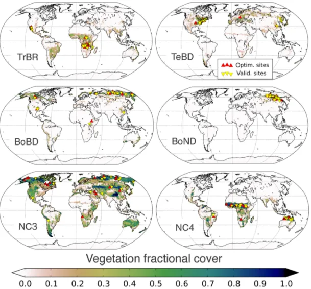
The six deciduous, non-agricultural PFTs of ORCHIDEE are optimised in this study. For each of the PFTs that were op-timised we selected 30 sites (where one site is equal to one model grid cell at 0.72◦resolution – see Sect. 2.4) that ful-filled several constraints (Fig. 2). First the grid cells have to be representative of the considered PFT and thus contain a high fraction of the PFT in question. This was mostly > 0.6 except for the boreal broadleaved deciduous (BoBD) PFT where the fractional cover is never greater than 0.4. For this PFT, all the grid points selected contained 40 % BoBD trees and high fractions (0.5–0.6) of natural C3 grasses (NC3); thus both PFTs were optimised for these grid cells simultane-ously. Second, the site locations should be as representative as possible of the PFT spatial distribution. This is achieved by a random sampling of grid cells with a fractional coverage above the given threshold. Lastly each NDVI time series was visually inspected and discarded if it was too noisy or

con-tained an incomplete seasonal cycle. Whilst we could not be 100 % certain that no land cover change or disturbance had taken place for the grid cells selected, none of the time series showed discernible signs of a shift in vegetation. A total of 15 of the sites were used in the optimisation, and the other 15 were kept for spatial validation following the optimisa-tions (see Fig. 2). To separate the 30 sites into 2 sets of 15 for optimisation and validation, we ordered all sites by their grid cell row number and took alternate points for each list.

2.4 Optimisations and simulations performed

In this study ORCHIDEE is used in forced offline mode and is driven by 3-hourly ERA-Interim meteorological fields (Dee et al., 2011), on a regular 0.72◦grid, which are linearly interpolated to a half hour time step within ORCHIDEE. We use the Olson land cover classification, which contains 96 classes at a resolution of 5 km, to derive the PFT frac-tions at 0.72◦following (Vérant et al., 2004). The soil texture classes are derived from Zobler (1986). The impact of land use change, forest management, harvesting and fires were not included in any simulation.

2.4.1 Multi-site optimisation

For each PFT optimised, the 15 optimisation sites (see Sect. 2.3.3) were first optimised simultaneously (i.e. all sites were included in the same cost function), over the 2000–2008 period using the multi-site (MS) approach detailed in Kuppel et al. (2012). Following (Santaren et al., 2014) we tested the ability of the algorithm to find the global minimum of the cost function by starting the iterative minimisation algorithm (see Sect. 2.3.1) at different points in the parameter space, choosing 20 random “first guess” sets of parameters and per-forming a MS optimisation for each. The results of these tests are presented in Sect. 3.1.

2.4.2 Single-site optimisation

A single site (SS) optimisation was then performed for each of the same 15 optimisation sites. The assimilations were ex-actly the same as for the MS optimisation, except each site was optimised separately. The posterior parameter vector re-sulting from the “best” random first guess MS optimisation (taken as the greatest % reduction in the cost function) was used as the first guess for the SS optimisation. The first guess with the greatest % reduction in the cost function was equiv-alent to the first guess that resulted in the lowest value of the cost function, as the % reduction was calculated using the value of the cost function using the default (prior) OR-CHIDEE parameters.

2.4.3 Site-based validation

The same MS posterior parameter vector for each PFT was then used to perform a simulation at each of the 15 extra

spatial validation sites (see Sect. 2.3.3) over the same time period. In addition, prior and posterior simulations at all 30 optimisation and validation sites were extended to cover the 2009–2010 period in order to perform a temporal validation.

2.4.4 Global-scale evaluation

Finally two global-scale simulations (with increasing atmo-spheric CO2concentration and changing climate) were

per-formed for the 1990–2010 period with both the prior and MS posterior parameter values, in order to evaluate the impact of the optimisation on the global mean patterns and trends in annual mean fAPAR, amplitude and GSL. The same ERA-Interim 0.72◦ forcing data were used as for the site-based optimisations. Note that no spinup of the soil C pools was needed for this study.

2.5 Post-processing and analysis

The prior and posterior RMSE and correlation coefficient, R, were calculated for both the MS and SS optimisations at all sites for a comparison. The values for the spatial and tempo-ral validation simulations were evaluated to assess the spatial and temporal generality of the posterior vectors. For all the analyses performed in this study, metrics given per PFT at global scale were derived for grid cells that contained > = a certain PFT fraction following the rules used to select the optimisation sites (see Sect. 2.3.3).

2.5.1 Calculation of the start of leaf onset and

senescence, GSL and trend analysis

The curve-fitting method of Thoning et al. (1989) was used to fit a function to the daily time series of observations and model output as described in Maignan et al. (2008). The function consists of two parts; a second-order polynomial that is used to account for the long-term trend, and a fourth order Fourier function to approximate the annual cycle. The residuals of the fit to this function were filtered with two low pass filters in Fourier space (80 and 667 cut-off days) and then added back to the function to produce a smoothed function that captures the seasonal and inter-annual variabil-ity and long-term trend. The detrended curve can be calcu-lated by subtracting the trend from the smoothed function. The start of season (SOS – leaf onset) and end of season (EOS – the start of leaf senescence) were defined as the up-ward and downup-ward crossing points of the “zero-line” of the de-trended curve per calendar year (see Fig. 1 in Maignan et al., 2008). These values were calculated for all grid cells with only one seasonal cycle per year (this includes grid cells in the SH where the growing season spans 2 calendar years). The GSL was calculated as the number of days per calendar year when the detrended curve is greater than zero. There-fore unlike the SOS and EOS, the GSL was also calculated for grid cells that contain multiple growing seasons within a calendar year.

Figure 2. Global distributions of fractional cover for the six PFTs optimised in this study. Red upright triangles mark the location of the

optimisation sites, and yellow upside-down triangles mark the location of the validation sites.

For the trend analysis, a linear least squares regression was used to calculate the long-term trend in the annual fAPAR amplitude, growing season length (GSL) and the mean fA-PAR time series.

2.5.2 Global evaluation with MODIS NDVI

The global simulations were evaluated with the same MODIS NDVI data that were used at the site level for the op-timisation, following the protocol of Maignan et al. (2011). The following metrics were used for evaluation of both the prior and posterior simulations.

The correlation between the normalised simulated fAPAR and MODIS NDVI weekly time series.

The bias (in days) between the modelled and observed SOS and EOS dates (model – observations) were also ex-amined so as to investigate the impact on the timing of the phenology more directly (a positive bias indicates the model date is later than the date calculated from the observations).

The above metrics were calculated for each grid cell. Fol-lowing this a global median value was calculated, as well as a median correlation per PFT.

3 Results

3.1 Convergence of the optimisation algorithm

We initially tested the ability of the MS optimisation to find the global minimum of the cost function (J (x)) by starting at 20 different random “first guess” points in the parameter space. For the forest PFTs and natural C3 grasses, the final cost function value was mostly within ∼ 30 % of the mini-mum (lowest) cost function value (up to 50 % for TeBD – Table 3, 2nd column), and in the majority of cases a 30– 60 % reduction in the cost function was achieved (Table 3, 3rd column). The skill of the optimisation algorithm is highly dependent on the PFT in question; the lowest final value of the cost function and the highest % reduction (normalised to

Table 3. Metrics to describe the ability of the optimisation

algo-rithm to find the global minimum of the cost function for the MS op-timisation using 20 different random “first guess” parameters. The 2nd column shows the final value (after 25 iterations of the BFGS optimiser) for the random test that resulted in the lowest value of J (x)(the cost function), which corresponds to the highest % reduc-tion in J (x). The 3rd column gives an indicareduc-tion of the distribureduc-tion of the final values for all 20 tests with respect to the lowest value ob-tained (given in column 1). This is represented as the difference be-tween the final value of J (x) for each test and the minimum value of J (x), divided by the same minimum value. The 4th column shows the % reduction of J (x) normalised to the value of J (x) for the de-fault parameters of ORCHIDEE. The two values for the 3rd and 4th columns represent the interquartile range (25th to 75th percentiles) for the spread across the 20 random tests.

PFT Minimum Fractional difference % Reduction

J (x) from J_min (J /Jb) TrBR 9720 0.24–0.25 44.1–44.6 TeBD 4730 0.2–0.5 28–44 BoBD 4260 0.07–0.32 54–63 BoND 2000 0.02–0.31 77–82 NC3 6590 0.08–0.34 29–44 NC4 19 160 0.03–0.1 4–11

the value of J (x) for the default parameters of ORCHIDEE) across all 20 random tests was seen for the BoND PFT. There was a higher spread in the % reduction for natural C3 grasses and the TeBD PFTs, suggesting the cost function is not as smooth (i.e. contains more local minima) as for the BoND PFT (for example). This is possibly linked to the need for a greater number of species for certain PFTs or due to differing parameter sensitivities under different climate regimes (the NC3 sites have a particularly wide global distribution). Nev-ertheless, examining these results we feel confident that for these PFTs the assimilation system converges to a value of the cost function that is reasonably close to the likely global minimum. Thus for the SS optimisations, the site-based val-idation and the global-scale evaluation we used the MS pos-terior vector that resulted in the minimum value of the cost function.

However the picture is different for natural C4 grasses (NC4). Only 2 out of the 20 random first guess tests resulted in a > 10 % reduction in the cost function, and although the spread of final values of the cost function was low and close to the minimum value (Table 3, column 2), the final value was between 2 and 10 times higher than that achieved for other PFTs (Table 3, column 1). This suggests that the optimisa-tion algorithm cannot find a better fit to the data than with the default parameter values. It is possible that the BFGS al-gorithm is not adequate for exploring the parameter space for NC4 grasses, but given that none of the random tests resulted in a noticeable reduction in the cost function, it is more likely that the model sensitivity to the parameters is lower than for

Figure 3. Time series (zoom to 2003–2007) for one example BoND

PFT site (72◦N, 120.24◦E) of (a) the normalised modelled total fA-PAR and MODIS NDVI data; (b) the un-scaled model total fAfA-PAR and MODIS NDVI data; (c) the corresponding modelled LAI for the BoND PFT only. The black curve corresponds to the MODIS NDVI data, the blue curve is the prior model simulation, the orange curve shows the model simulation using the posterior parameters from the SS optimisation, and the red curve corresponds to the model sim-ulation at this site using the MS posterior parameter values. The prior and posterior RMSE and R are given in the upper left box. The MODIS NDVI and model fAPAR time series were normalised to their maximum and minimum value over the 2000–2008 period for the optimisation (see Sect. 2.2.1).

other PFTs. This in turn suggests that the phenology model structure itself is inadequate for this NC4 grasses.

3.2 Improvement in the model–data fit at the site level

3.2.1 Temperate and boreal PFTs

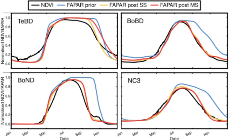
There is an improvement in the model–data fit after both SS and MS optimisations for all temperate and boreal broadleaved and needleleaved deciduous forests (TeBD, BoND, BoBD) and for natural C3 grasses (NC3), largely re-sulting from an earlier onset of senescence in the model and therefore a substantially shortened growing season length (Figs. 3 and 4). The shift in the start of leaf growth is much smaller, which is not surprising as the prior model more closely matches the observations. Of the four PFTs listed above, only TeBD trees have a slightly later leaf onset as a result of the optimisation. Figure 3 shows the full time se-ries at one site of both the normalised and un-normalised fAPAR and NDVI, together with the simulated LAI, for the BoBD PFT. This site is provided as an example of the typ-ical changes in temporal behaviour seen for the four PFTs listed above. Figure 4 shows the mean seasonal cycle of the normalised fAPAR/NDVI across all sites and years (2000– 2008) for each of the four PFTs and demonstrates that the patterns seen in Fig. 3 are similar for all the boreal and tem-perate deciduous PFTs.

Jan Mar May Jul Sep Nov Date 0.0 0.2 0.4 0.6 0.8 1.0 N or m al ise d N D V I/f A PA R

NDVI FAPAR prior FAPAR post SS FAPAR post MS

Jan Mar May Jul Sep Nov

Date 0.0 0.2 0.4 0.6 0.8 1.0 N or m al ise d N D V I/f A PA R

NDVI FAPAR prior FAPAR post SS FAPAR post MS

Jan Mar May Jul Sep Nov

Date 0.0 0.2 0.4 0.6 0.8 1.0 N or m al ise d N D V I/f A PA R

NDVI FAPAR prior FAPAR post SS FAPAR post MS

Jan Mar May Jul Sep Nov

Date 0.0 0.2 0.4 0.6 0.8 1.0 N or m al ise d N D V I/f A PA R

NDVI FAPAR prior FAPAR post SS FAPAR post MS

TeBD BoBD

BoND NC3

Jan Mar May Jul Sep Nov

Date 0.0 0.2 0.4 0.6 0.8 1.0 N or m al ise d N D V I/f A PA R

NDVI FAPAR prior FAPAR post SS FAPAR post MS

Jan Mar May Jul Sep Nov

Date 0.0 0.2 0.4 0.6 0.8 1.0 N or m al ise d N D V I/f A PA R

NDVI FAPAR prior FAPAR post SS FAPAR post MS

Figure 4. The mean seasonal cycle of the normalised modelled

fA-PAR before and after optimisation, compared to that of the MODIS NDVI data, for the temperate and boreal deciduous PFTs (TeBD, BoBD, BoND and NC3). Black = MODIS NDVI data; blue = prior model; orange = single-site optimisation; red = multi-site optimisa-tion.

The optimisations resulted in a significant reduction in the RMSE (34–61 %) and increase in correlation (poste-rior R > 0.82) between the normalised modelled fAPAR and MODIS NDVI data for all four temperate and boreal PFTs (Table 4). The variation in the RMSE and R at each site for prior, multi-site optimisation and the spread for all the single-site optimisations for all four PFTs are shown in Fig. S1 in the Supplement. The improvement is greatest for the Boreal PFTs (median reduction in RMSE across all sites for both SS and MS optimisations of ∼ 50–60 % and an increase in

R from 0.41 to 0.9), but nonetheless the optimisations of the temperate broadleaved deciduous (TeBD) and natural C3 grasses (NC3) PFTs result in a median reduction of uncer-tainty of between ∼ 20–40% and an increase in R of up to

∼0.2.

There is a discernible slowing down in the rate of leaf growth towards the end of the leaf onset after the assimila-tion, which particularly results in an improved fit to the ob-servations for the TeBD, BoND and NC3 PFTs. However it is noticeable that although parameters that partially control the rate of leaf growth and fall are included in the optimisation, the model generally grows and sheds leaves too fast com-pared to the observations, except for the BoBD PFT, which results in the model having an unnatural “box-like” temporal profile (Fig. 4 and see Sect. 4.3 for further discussion).

The MS optimisation (red line in Figs. 3 and 4) largely results in a similar reduction in RMSE and increase in R as the SS optimisations at each individual site except for TeBD trees, although a similar magnitude of improvement is achieved for this PFT as for the others (Table 4 and Fig. S1). This suggests that the MS parameter vector is uni-versal enough to be used to perform global simulations.

T able 4. Prior and posterior median (across sites) RMSE and R (and median reduction of RMSE in % in brack ets) for the 15 sites included in the optimisation and for the 15 sites used for spatial v alidation, for each PFT . F or the temporal v alidation all 30 sites are included, b ut only for the 200–2010 period. F or the spatial and temporal v alidation, the posterior MS parameter v ector w as used. PFT Optimisation Spatial v alidation T emporal V alidation Prior RMSE SS Post RMSE M S Post RMSE Prior R SS Post. R MS Post. R Prior RMSE Post RMSE Prior R Post. R Prior RMSE Post RMSE Prior R Post. R T rBR 0.29 0.18 (39) 0.22 (24) 0.73 0.87 0.82 0.28 0.18 (32) 0.76 0.88 0.28 0.18 (33) 0.75 0.88 T eBD 0.20 0.12 (39) 0.16 (21) 0.90 0.97 0.93 0.20 0.16 (19) 0.91 0.94 0.20 0.17 (18) 0.92 0.94 BoBD 0.30 0.14 (57) 0.14 (52) 0.54 0.91 0.91 0.29 0.15 (47) 0.59 0.89 0.31 0.23 (26) 0.56 0.67 BoND 0.39 0.15 (61) 0.16 (57) 0.41 0.90 0.89 0.38 0.16 (59) 0.42 0.90 0.39 0.16 (58) 0.40 0.88 NC3 0.31 0.20 (34) 0.20 (32) 0.62 0.82 0.85 0.30 0.22 (26) 0.65 0.77 0.31 0.21 (35) 0.61 0.79 NC4 0.23 0.21 (11) 0.24 (0) 0.81 0.82 0.81 0.24 0.23 (7) 0.75 0.79 0.24 0.23 (3) 0.80 0.86

2003 2004 2005 2006 Date -0.2 0.0 0.2 0.4 0.6 0.8 1.0 1.2 N or m al ise d N D V I/f A PA

R NDVIFAPAR prior

FAPAR posterior SS FAPAR posterior MS 0 20 40 60 80 100 120 140 P re ci pi ta tio n (m m ) Sim RMSE R Prior 0.204 0.85 SS posterior 0.191 0.88 MS posterior 0.225 0.85 2003 2004 2005_Date 2006 -0.2 0.0 0.2 0.4 0.6 0.8 1.0 1.2 N or m al ise d N D V I/f A PA

R NDVIFAPAR prior

FAPAR posterior SS FAPAR posterior MS 0 10 20 30 40 50 P re ci pi ta tio n (m m ) Sim RMSE R Prior 0.306 0.66 SS posterior 0.181 0.82 MS posterior 0.179 0.84 ! TrBR ! ! NC4! (a) (b)

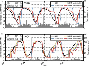
Figure 5. Example time series (2002–2008 period) for the

trop-ical deciduous PFTs for which phenology is driven by moisture availability. The two panels compare the normalised simulated fAPAR to the normalised MODIS NDVI (black curve) prior to (blue curve) and after the optimisations (orange curve = SS opti-misations; red curve = MS optimisation) for a (a) TrBR tree site (5.77◦S, 25.92◦E) and a (b) NC4 grass site (10.08◦N, 4.32◦W). The prior and posterior RMSE and R are given in the upper left boxes. The grey vertical lines show the daily precipitation.

3.2.2 Tropical deciduous forest and C4 grasses

For both the tropical broadleaved raingreen (TrBR) and nat-ural C4 grass (NC4) PFTs, the median prior fAPAR simula-tion performs reasonably well compared to the observasimula-tions, with RMSEs of 0.29 and 0.23 and R of 0.73 and 0.81, respec-tively (Table 4 and Fig. S1). Following optimisation there is an improvement in the median model–data misfit both for the SS and MS optimisation for TrBR trees across all sites, but the spread in posterior RMSE and R values remains high (Fig. S1). Figure 5a shows an example of the typical issues seen for some TrBR sites that have not been resolved by op-timising the phenological parameters. The growing season is always slightly out of phase, even after the optimisation, with the simulated SOS and EOS lagging that of the obser-vations. The observed start of leaf growth coincides with the start of increased precipitation, as would be expected, but the simulated onset does not, despite the fact that the onset phe-nology model is solely driven by soil water availability. Pos-sible causes of inconsistencies in the model will be discussed in Sect. 4.4. At the end of the growing season the optimisa-tion results in a more gradual start of leaf turnover at many sites, thus better matching the observation temporal profile, but still the end of the leaf fall lags that of the observations (Fig. 5a). Finally at some of the sites the observations show a smaller, second period of growth in some years (not shown), but the model also does not capture this.

There is no change in the median RMSE and R for the NC4 PFT with the MS optimisation, although the prior model–data misfit is relatively small (Fig. S1). The SS opti-misations do result in a small reduction in the median RMSE (0.21) but no improvement in the median correlation. This is not surprising given the results of the random first guess tests presented in Sect. 3.1. A comparison of the observed and modelled time series of NDVI and fAPAR at each site again reveals where the model is not able to fully reproduce the seasonality seen in the observations. At many sites the model predicts a positively biased (i.e. too late) SOS, followed by a drop in fAPAR in the first half to middle of the year that is not seen in the observations, and does not correspond to a decline in precipitation (e.g. Fig. 5b). The optimisation can result in the partial removal of this feature, particularly for SS optimisations at certain sites, but at the expense of a further delay to the start of leaf growth. Neither the SS or MS opti-misations are able to reduce the model–data misfit by forcing an earlier start of senescence at any of the sites. As there is no discernible improvement after the MS optimisation of the NC4 PFT, the posterior parameters are not used in the further analysis of global changes to the gross primary productivity (GPP), GSL or trends. It is likely that the phenology models that are used in water limited ecosystems (TrBR and NC4) need revising (see discussion in Sect. 4.4).

3.3 Validation of the optimised phenology

3.3.1 Spatial and temporal validation

Table 4 also shows the RMSE and R for the extra 15 sites that were not included in the optimisation (spatial valida-tion), and for all sites for the period 2009–2010 that were not included in the optimisation (temporal validation). These validation exercises were performed with just the MS poste-rior parameter vector for each PFT. Similar magnitudes and patterns of improvement are observed between the PFTs as for the sites used for optimisation – the largest improvement is seen for the BoND PFT, and there is no improvement for NC4 grasses. These results again give confidence in the gen-erality of the MS posterior vector and its use in regional and global scale simulations, except for the NC4 PFTs for which there was an insufficient improvement post-optimisation.

3.3.2 Validation at global scale with MODIS NDVI

The global median correlation between the model and the MODIS NDVI data have increased from 0.56 to 0.67 after the optimisation, demonstrating an overall improvement in the simulated fAPAR time series. As seen at the site level, the largest increase in correlation between the modelled and observed time series is for the boreal PFTs. There is also a modest improvement for natural C3 grasses (Table 5). Fig-ure 6 shows the spatial distribution of the correlation for the both posterior simulation and the difference after

optimisa-Table 5. Median prior and posterior correlation between

mod-elled fAPAR and satellite NDVI daily time series and inter-annual anomalies of the annual mean. The metrics are computed for each PFT for grid cells that contained > = fraction that was used to select the sites for the PFT in question (see Sect. 2.3.3).

PFT Time series correlation IAV correlation Prior Posterior Prior Posterior

TrBE 0.18 0.19 0.21 0.13 TrBR 0.71 0.85 0.31 0.29 TeNE 0.29 0.44 0.30 0.42 TeBE 0.32 0.19 0.54 0.44 TeBD 0.88 0.89 0.30 0.44 BoNE 0.35 0.45 0.25 0.22 BoBD 0.52 0.86 0.48 0.40 BoND 0.33 0.81 0.02 0.13 NC3 0.56 0.76 0.29 0.32 NC4 0.70 0.74 0.30 0.30 AC3 0.36 0.35 0.49 0.50 AC4 0.48 0.48 0.33 0.35

tion (posterior – prior). The difference map shows that R has mainly improved for boreal regions in the north of Canada and in Siberia, the C3 grasslands in central Asia and west-ern North America, and the high altitude regions of the An-des (due to improvements in BoBD, BoND and NC3 PFTs) with slight changes for tropical raingreen trees in savannah-dominated regions in Africa. A decrease in R was seen in part of the drylands of western North America and along the western boundary of South America.

The global median end of season (EOS) bias (model – observations) between the model and MODIS data was re-duced dramatically as a result of the optimisation (prior: 33 days; posterior 5 days). Note that a positive bias indicates the model date is later than the date derived from the MODIS data. Again, boreal PFTs and NC3 grasses showed consider-able improvement, as expected from the site-level behaviour (Sect. 3.2), but grid cells containing high fractions of temper-ate and boreal evergreen trees were also positively affected (Table 6). The bias in the start of season (SOS) dates also decreased (prior and posterior global median bias of 22 and 14 days, respectively), with improvements seen for all PFTs except TeBD trees and crops (Table 6).

3.4 Posterior parameters and processes constrained

The prior value, prior range and posterior value from the MS optimisation for each parameter (per PFT) are shown in Ta-ble 2. Figure 7 shows the prior and posterior parameter values for both the SS and MS optimisation for each parameter and each PFT. In Fig. 7 the mean and standard error of the mean of the SS posterior parameters are shown (circle with error bars), together which the value obtained at each individual site (crosses). For the prior simulation and MS optimisation

Table 6. Median prior and posterior bias between model- and

observation-derived start of season (SOS) and end of season (EOS) dates (model – observations). The metrics are computed for each PFT for grid cells that contained > = fraction that was used to select the sites for the PFT in question (see Sect. 2.3.3). A negative bias indicates the modelled date is earlier than the one calculated from the observations.

PFT SOS bias EOS bias

Prior Posterior Prior Posterior

TrBE 20 −3 −146 −3 TrBR 30 13 9 12 TeNE 38 20 41 −33 TeBE 70 49 42 −4 TeBD 4 6 14 13 BoNE 38 29 52 13 BoBD 18 10 43 8 BoND 5 1 36 2 NC3 25 15 42 −1 NC4 32 15 −7 −2 AC3 −17 −17 19 18 AC4 8 8 18 18

the error bar corresponds to the standard deviation of the pa-rameter value (calculated using Eq. 3). The MS uncertainty is lower than spread of SS posterior values, suggesting that it underestimates the true uncertainty of the posterior parame-ters. This may be the case given the assumptions of linearity of the model and of Gaussian and uncorrelated errors.

The lower posterior values of Kpheno_critreduced the

pos-itive bias in the SOS dates, for temperate and boreal decid-uous trees and natural C3 grasses, thus providing a better fit to the model. For all temperate and boreal PFTs the poste-rior value of the Klai_happyparameter, which is used to

calcu-late the LAI value below which leaf growth is supported by the carbohydrate reserves, decreases for both the SS and MS optimisation. In ORCHIDEE the rate of leaf growth slows down after this LAI threshold is reached as the C now comes from photosynthesis, which may be limited by various fac-tors. Lower values of Klai_happytherefore result in an earlier

end to the period of rapid canopy growth at the beginning of the season and thus a smoother temporal profile follows dur-ing the final stages of growth. This partially compensates for the “box-like” model behaviour, but structural deficiencies related to spatial variability need to be addressed further (see Sect. 4.3). The lower value of Klai_happy (together with the

earlier start to senescence) is also responsible for the reduc-tion in the peak LAI at some sites for some PFTs, particularly BoND trees (see Fig. 3 for example). It may be hypothesised that the optimisation resulted in a reduction in the C allocated to the carbohydrate reserve, which therefore may also have contributed to the decrease in the peak LAI. However an ex-amination of the simulated carbohydrate reserve showed this not to be the case (results not shown). In any case this

ob-Figure 6. Global maps showing the correlation between the simulated fAPAR and MODIS NDVI data in the weekly time series for the

posterior simulation (left column) and the difference after optimisation (posterior – prior) (right column). Note POST refers to the posterior simulation after optimisation, and PRIOR to the simulation using the standard parameters of ORCHIDEE.

served reduction in peak LAI was not a common result of the optimisation when considering all PFTs.

The earlier start of senescence is overwhelmingly caused by an increase of Tsenesfor all temperate and boreal trees and

natural C3 grasses in both the SS and MS optimisations, as well as a lowering of the critical leaf age (Lagecrit), though

this is not the case for BoBD trees (Fig. 7). It is important to remember however that the optimisations at BoBD sites also included high fractions of natural C3 grass that were op-timised at the same time (see methods Sect. 2.3.3) and there-fore the same parameter can have strong interactions between the two PFTs, as can be seen in for the Lagecritparameter in

the correlation matrices in Fig. S2. The Lfallparameter has

not changed considerably after the optimisation, suggesting that the rate of leaf fall matches that of the observations when parameters that govern the start of leaf senescence have been optimised. However, one exception to this is seen for TeBD trees, where the rate of leaf fall has decreased following op-timisation (Fig. 4a), and thus the model better matches the observations.

The phenology of C3 grasses is also controlled by soil moisture availability. The moisture-related leaf onset param-eter, MoistTmin, does not appear to be as important as the

temperature-related leaf onset parameter (Kpheno_crit).

How-ever, the increase in the value of both Tsenesand Moistsenes

post-optimisation show that both moisture and temperature conditions are responsible for the marked shortening of the growing season length for natural C3 grasses (Fig. 4), as would be expected given the wide geographical distribution of this PFT.

For the tropical raingreen forests (TrBR), there is a de-crease in the posterior SS and MS values of MoistTminand

an increase for the Moistsenesparameter, which results in an

earlier start of both leaf growth and senescence, again reduc-ing the positive bias in the SOS and EOS dates predicted by the model. However the parameters are “edge-hitting”, which

suggests the optimisation has not necessarily found the opti-mum solution. This may explain why the model remains out of phase with the observations as described above (Fig. 5a).

Although the phenology of C4 grasses is governed by both temperature and moisture conditions, the fact that there is no change in the value and uncertainty of the temperature-related parameters, Kpheno_critand Tsenesshows a lack of

sen-sitivity to both (Fig. 7), which is not surprising as the location of the C4 grasses pixels used in this study are mainly located in moisture-limited tropical regions. The SS and MS poste-rior values of the moisture-related parameters, MoistTminand

Moistsenes,have changed (increased), but the spread of the

SS optimised parameter values is large, which accounts for the lack of improvement in the median RMSE and correla-tion between the time series of the model and observacorrela-tions (Table 4).

3.5 Change in global patterns and trends of mean

annual fAPAR, amplitude and GSL

Figure 8 shows the change (posterior – prior) in the mean annual GSL, fAPAR amplitude and mean simulated fAPAR globally over the 1990–2010 period. As expected from the site-level results for temperate and boreal PFTs (Fig. 4 and Table 4), there was a strong decrease in the mean GSL in the high latitudes and grasslands across much of the NH (median of −30 and −10 days for boreal (60–90◦_{N) and} temperate (30–60◦_{N) regions, respectively), as well as in} equatorial Africa (median of −28 days) (Fig. 8a). An in-crease in the GSL of ∼ 7 days was mostly observed in the Sahel and Miombo savannah regions of Africa. A decrease in fAPAR amplitude was also seen in Siberia and in water-limited grasslands in southern Africa, the western United States and central Asia (Fig. 8b). Although the primary aim of the assimilation was to constrain the timing of the phe-nology, changes in the amplitude are the result of the

inter-TrBR! TeBD!BoBD!BoND!

NC3!

NC4!

0.35 0.40 0.45 0.50 0.55 0.60 0.65 10 20 30 40 50 20 40 60 80 100 120 140 0.1 0.2 0.3 0.4 0.5 0.6 0.7 0.8 0.8 1.0 1.2 1.4 1.6 0.35 0.40 0.45 0.50 0.55 0.60 0.65 10 5 0 5 10 15 20 10 20 30 40 50 0.8 1.0 1.2 1.4 1.6 0.35 0.40 0.45 0.50 0.55 0.60 0.65 10 5 0 5 10 15 20 10 20 30 40 50 0.8 1.0 1.2 1.4 1.6 0.35 0.40 0.45 0.50 0.55 0.60 0.65 10 5 0 5 10 15 20 10 20 30 40 50 0.8 1.0 1.2 1.4 1.6 0.35 0.40 0.45 0.50 0.55 0.60 0.65 10 5 0 5 10 15 20 0.3 0.4 0.5 0.6 0.7 0.8 0.9 1.0 20 40 60 80 100 120 140 0.8 1.0 1.2 1.4 1.6 0.35 0.40 0.45 0.50 0.55 0.60 0.65 10 5 0 5 10 15 20 20 40 60 80 100 120 140 0.3 0.4 0.5 0.6 0.7 0.8 0.9 1.0 60 80 100 120 140 160 180 200 220 240 60 80 100 120 140 160 180 200 220 240 60 80 100 120 140 160 180 200 220 240 60 80 100 120 140 160 180 200 220 240 60 80 100 120 140 160 180 200 220 240

L

ag e cri t!

K

p h e n o _ cri t!

K

lai_happy !

T

se n e s!

L

fall !

Mo

ist

T mi n !

Mo

ist

se n e s, n o se n e s! 240! 60 80 100 120 140 160 180 200 220 240 80! 1.8! 0.8! 0.7! 0.4! 20! -10! 50! 10! 140! 20! 0.8! 0.1! 0.3! 1.0! 140! 20!

Figure 7. The prior (blue), MS posterior (red) and SS posterior

(or-ange) parameter values (circles) and uncertainty (error bars – vari-ance calculated in Eq. 3) for each parameter and each PFT. For the SS optimisations the circle and error bars represent the mean and standard error of the mean of all sites, and the crosses give the posterior values for each site. Refer to Table 1 for a description of the PFTs and Fig. 1 and Appendix A for a description of each parameter. The y axis range represents the maximum upper and lower bounds for each parameter across all PFTs, and the horizontal dashed lines represent the parameter range for each individual PFT.

play between parameters controlling the rate of leaf growth and fall and the timing of senescence that ultimately result in a lower maximum LAI, as discussed in Sect. 3.4. The com-bined result was a strong decrease in the annual mean fAPAR in most regions of the globe that are not dominated by ever-green trees, crops or bare soil, except for the Sahelian region in Africa (Fig. 8c).

Figure 9 shows the linear trend (yr−1)in the annual mean fAPAR for the 1990–2010 period, both for the prior and pos-terior simulation and their difference. The trends of the an-nual mean are shown as it is a more comprehensive met-ric compared to the daily/monthly time series of fAPAR, the GSL or fAPAR annual amplitude. The large-scale spatial

(b)!

(a)!

(c)!

Figure 8. The difference (posterior – prior) of the simulated annual

mean (over the 1990–2010 period) (a) GSL (days); (b) amplitude of the normalised fAPAR (range 0–1) and (c) mean normalised fA-PAR.

patterns of positive and negative trends over the 1990–2010 period were not altered significantly after the assimilation, however the strength of the trend is generally reduced. This can be seen in Fig. 9 as positive “greening” trends mostly correspond to regions where there was a decrease in the slope of the trend after optimisation (orange areas in Fig. 9c), and vice versa for negative “browning” trends (purple areas in Fig. 9c). This was not always the case however, for example the “greening” trend in central Siberia (around 60◦N) and the “browning” trend in parts of the Sahelian both increase

in strength following the assimilation. Note that an examina-tion of the trends in other metrics (SOS, EOS, GSL or annual amplitude) did reveal different changes in the spatial patterns following the assimilation. For example the increase in GSL actually increased slightly in north-western Siberia, and the decline in GSL in Mongolia (also seen as a browning trend in the annual mean in Fig. 9) increased by ∼ 2–3 days after the optimisation (results not shown). Further details are not discussed here.

We chose not to compare the simulated trends with that of the MODIS NDVI. This was partly because the 2000–2010 period is likely too short to calculate a robust trend, as the influence of inter-annual variability will be stronger; indeed the trends over the longer 1990–2010 period are more geo-graphically distinct. Secondly it was not the aim of this study to validate the modelled trends, nor would it be appropriate, because we have used a version of the model that does not in-clude land use change, disturbance and other effects that will contribute to changes in vegetation greenness at global scale. The results presented here serve to highlight that different parameter values can change the strength, sign and location of the trends. However, it is worth noting that the sign of the simulated trend does not always match the MODIS data, especially for drier, warmer semi-arid regions. For example, the browning trend seen in the Kazakh Steppe in the MODIS data is stronger in ORCHIDEE and extends further east into Mongolia (results not shown). Similarly, the model predicts a decline in fAPAR across much of sub-Sahelian Africa that is not seen in the MODIS NDVI. The optimisation did not re-sult in a change in the trend direction for this region, though generally it did reduce its strength. Overall the greening trend in the NH (> ∼ 30◦_{N) was well captured by the model both} before and after optimisation.

4 Discussion

4.1 Optimisation performance

Whilst the SS optimisations result in a reduction in the model–data misfit across a range of sites, this study has shown that a MS optimisation can achieve a similar improve-ment with one unique parameter vector. This is an important result, and reinforces the conclusions of Kuppel et al. (2014) that the MS posterior parameters can be used with confidence to perform global simulations. Previous site-level optimisa-tions of phenology models have resulted in a wide range of parameterisations of growing degree day sum, chilling re-quirements and light availability (Migliavacca et al., 2012; Richardson and O’Keefe, 2009); therefore it is difficult to know which values to use for regional-to-global scale simu-lations. In most cases the MS optimisation averages out the variability due to specific site characteristics. The validation at the site and global scale using daily MODIS NDVI data demonstrates the generality of the MS posterior parameter

Figure 9. Linear trend (yr−1)in the annual mean of the simulated

normalised fAPAR for the 1990–2010 period: (a) prior simulation;

(b) posterior simulation; (c) difference between the prior and

poste-rior (posteposte-rior – pposte-rior).

vectors given the ORCHIDEE model structure. This gives confidence in using these values in regional-to-global scale simulations of the carbon and water fluxes and for future pre-dictions with this model.

Although the optimisation resulted in a dramatic improve-ment in the seasonal leaf dynamics for temperate and boreal

ecosystems, the impact in the inter-annual variability (IAV) as a result of the optimisation for any variable – mean an-nual fAPAR, mean spring/autumn fAPAR, GSL, SOS, EOS – was minimal (results not shown). This was disappointing as generally there is a low correlation in the IAV between OR-CHIDEE and the MODIS data, and IAV in spring phenology has been shown to be a dominant control on C flux anomalies (Keenan et al., 2012).

4.2 Validity of the posterior parameters and optimised

phenology models

As data assimilation schemes are expected to result in a re-duction in the prior data–model misfit it is useful to assess if the posterior parameter values are indeed realistic, which is conditioned on the prior range as well as the interaction (cor-relation) between the parameters. However validating these values remains difficult, as there is no database that corre-sponds directly to phenology model parameters, which may have a different meaning in different models.

Leaf lifespan (LL) however can more easily be measured and therefore can be found in the literature and in plant trait databases (Kattge et al., 2011; Wright et al., 2004). Although leaf lifespan is not the same as the critical age for senes-cence parameter (Lagecrit), the leaf lifespan should be

sim-ilar if not lower than Lagecrit, and thus serves as a benchmark

to a certain degree. Reich (1998) gave 4–6 months for cold-temperate and boreal broadleaved and needleleaved decidu-ous trees, similar to the mean values for the same functional types in the TRY database (Kattge et al., 2011). These values encompass the range of optimised values for temperate and boreal broadleaved (TeBD and BoBD) PFTs (160 and 240 days, respectively, Table 2). The posterior value of Lagecrit

for the boreal needleleaved (BoND) PFT was lower than this range at 90 days, and was at the lower boundary of the pa-rameter range. The TRY database gives a mean value of 3.85 and 1.68 months for C3 and C4 grasses, respectively (Kattge et al., 2011). These values are higher than the posterior value of the C3 grasses (60 days) and lower than the posterior value for C4 grasses (166 days). The values of Lagecritfor NC3 and

BoND PFTs were therefore too low and it is also notable that the values of Tseneswere also at their upper bounds for these

two PFTs.

Most of the posterior values for the moisture-related phe-nology parameters for the tropical broadleaved raingreen and natural C4 grasses (TrBR and NC4) PFTs were also at their upper or lower bounds, even with liberal parameter bounds due to lack of prior knowledge. For example the posterior value of MoistTmin, the number of days since the last

mois-ture minimum before leaf onset, was unrealistically low at 10 days for TrBR trees. In turn the threshold of relative soil moisture needed for senescence (Moistsenes)was 0.8 and

0.7 % for TrBR and NC4 PFTs, respectively, which is likely too high. Assuming the prior range of the parameters does encompass the likely variability, such “edge-hitting”

poste-rior parameter values can indicate that other processes may be missing. Indeed certain studies (Galvagno et al., 2013; Rosenthal and Camm, 1997) have suggested that photope-riod is also important in determining autumnal senescence in deciduous conifers (e.g. BoND PFT). Possible deficiencies in the models that control tropical deciduous phenology are discussed further in Sect. 4.4.

In order to better evaluate the model parameterisa-tions, we suggest that the phenology observation and mod-elling community could engage in an elicitation exer-cise (O’Hagan, (1998, 2012); http://www.tonyohagan.co.uk/ shelf/). This would involve gathering knowledge on param-eter ranges of typical phenological model paramparam-eters from experts in the field, in order to derive probability distribu-tions of the parameter values. However, even if this exercise is carried out, measurements made at the species and site lev-els will be difficult to scale across species and to the coarse resolution used in TBMs.

The onset models used for temperate and boreal PFTs in ORCHIDEE are mostly simple spring warming models, though some include a chilling requirement (Table 1). Their comparative ability to reproduce the observations could add to evidence that more complex representations including light availability may not be needed (Fu et al., 2012; Picard et al., 2005; Richardson and O’Keefe, 2009). Other studies however have showed improved performance when a pho-toperiod term was included for species with a late leaf on-set (Hunter and Lechowicz, 1992; Migliavacca et al., 2012; Schaber and Badeck, 2003). Several authors (e.g. Fu et al., 2012; Linkosalo et al., 2008) have pointed out that whilst the simple warming onset models may perform well under cur-rent climate conditions, future predictions may require ad-ditional complexity; for example the model-defined chilling period may not be sufficient in warmer conditions. More im-portantly perhaps, any model that requires a fixed start date from which thresholds are calculated may be inconsistent under increased temperatures, as warming will start before the defined start date (Blümel and Chmielewski, 2012). Ide-ally therefore these models should also be tested under fu-ture warming scenarios, although (Wolkovich et al., 2012) showed the magnitude of species’ phenological response to temperature increases is lower in warming experiments com-pared to historical observations.

4.3 Accounting for spatial variability

The coarse-resolution observations used in this study will include the spatial variability in the timing of phenological events for different species within a PFT, or even due to spe-cific site characteristics (edaphic conditions, terrain/slope, local meteorological effects) within the same species (Fisher and Mustard, 2007). During senescence in particular, spatial variability in the rate of leaf fall, and to some extent the leaf colouration, will likely contribute to the decline in “green-ness” seen in NDVI observations. ORCHIDEE does not