AN ANALYSIS OF EXPOSURE PANEL DATA COLLECTED AT MILLSTONE POINT, CONNECTICUT
Russell T. Brown Stephen F. Moore Energy Laboratory
Ai ANALYSIS OF EXPOSURE PANEL DATA COLLECTED AT MILLSTONE POINT, CONNECTICUT
by Russell T. Brown and Stephen F. Moore Energy Laboratory and
Ralph M. Parsons Laboratory for
Water Resources and Hydrodynamics Department of Civil Engineering Massachusetts Institute of Technology
Cambridge, Massachusetts 02139 and
Resource Management Associates Lafayette, California 94549
sponsored by
Northeast Utilities Service Company New England Power Service Company
under the
MIT Energy Laboratory Electric Power Program
Energy Laboratory Report No. MIT-EL 77-015
TABLE OF CONTENTS
Page ACKNOWLEDGMENTS iii FOREWORD v 1.0 INTRODUCTION 1 1.1 Organization of Report 1 1.2 Background 21.2.1 Purposes for Ecological Studies 2
1.2.2 Ecological Studies of Millstone Point 3
1.2.3 Data Analysis Problems 6
1.3 Objectives of This Study 8
2.0 DESCRIPTION OF ON-GOING MILLSTONE POINT EXPOSURE PANEL STUDIES 9
2.1 Field and Laboratory Procedures 9
2.2 Existing Data Analysis 13
3.0 AN ECOLOGICAL BASIS FOR EXPOSURE PANEL DATA ANALYSIS 15 3.1 Some Dimensions of the Analysis Problem 15 3.1.1 Species Abundance Distributions: A Pessimistic Note 20 3.2 Ecological Processes Affecting Exposure Panels 23
3.2.1 Island Colonization 25
3.2.2 Accounting for Variability in Colonization 27
3.3 Shortcomings of the Island Model 28
3.4 Additional Considerations 31
3.4.1 Exposure Panel Community Structure 31
3.4.2 Frequency of Species Occurrence 33
4.0 STATISTICAL ANALYSIS OF THE TOTAL NUMBER OF SPECIES (S T) ON
12-MONTH PANELS 34
4.1 Description of Available Data 34
4.1.1 Taxonomic Standardization Procedures 40 4.2 Statistical Characterization of Samples 43
4.3 Statistical Comparison of Samples 46
4.3.1 Parametric Hypothesis Testing 47
Page
4.3.2 Non-Parametric Hypothesis Testing 54
4.3.3 Time Series Analysis 56
4.4 Comparison of 12-Month Samples with Panels of Other
Exposure Length 66
4.4.1 Analysis of Total Number of Species Occurring on
1-month Exposure Panels 70
5.0 COMMUNITY COMPOSITION ANALYSIS OF 12-MONTH EXPOSURE PANEL DATA 74
5.1 Cumulative Species Pool Analysis 74
5.2 Multivariate Analysis of Exposure Panel Data 78 5.2.1 Extensions of Elementary Statistics 80
5.2.2 Cluster Analysis 84
5.2.3 Factor Analysis 86
5.3 Species Presence/Absence Similarity Analysis:
Preliminary Results 87
5.3.1 Composition Analysis of Selected Taxonomic Sub-Groups 90 6.0 EVALUATION OF EXPOSURE PANEL STUDIES AT MILLSTONE 92
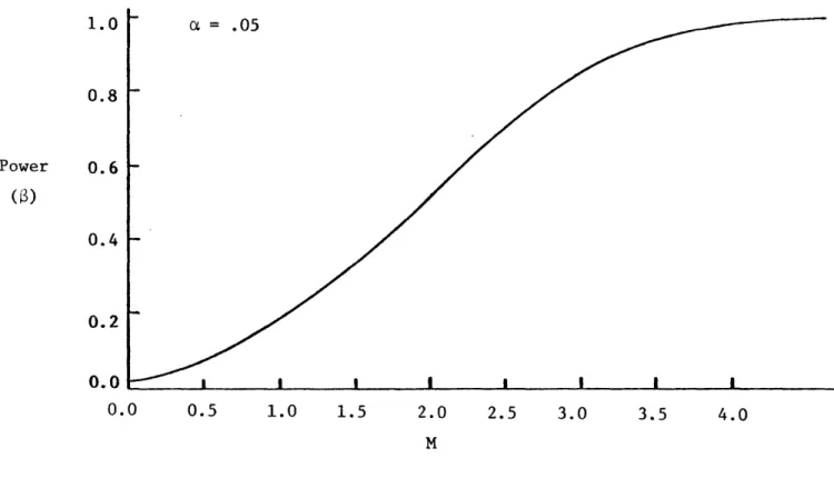
6.1 Power Analysis 92
6.1.1 Statistical Description of Power Analysis 93 6.1,2 Power Analysis Results for the t-test and F-test 102
7.0 SUMMARY, CONCLUSIONS AND RECOMMENDATIONS 107
7.1 Conclusions 109
7.2 Recommendations 111
8.0 REFERENCES 112
ACKNOWLEDGMENTS
This report represents the culmination of a three-year research effort, to which many people have contributed. Many changes have taken place among people involved and specific acknowledgment of each contributor during the three-year period is a formidable task. In expressing our thanks to those who have assisted us along the way, we apologize for any omissions we make.
Dr. Bill Renfro, Northeast Utilities Service Company, has been a steady source of encouragement, technical review and financial support. Mr. Brad
Schrader, at one time a student associated with this work and now with New England Power Service Company, has been a strong supporter technically and financially.
Various other persons at both NUSCO and NEPCO have periodically contributed their time and ideas in reviewing and guiding the progress of this research effort. Their efforts have been invaluable in helping us grapple with the confusion of the "real world."
Dr. Bob Hillman, Dr. Dave Cooper and other persons at the Battelle Columbus William F. Clapp Laboratories, Duxbury, Massachusetts, have made
essential contributions to our work. Not only have they made valuable technical contributions and helped us sort out our understanding of the ecology of
exposure panels, they also provided us without charge the data upon which this research is based. Without their assistance this research would not have been possible.
Many persons contributed to the notion of using the island colonization "model" described in Section 3. In particular, Mr. Charles Puccia, MIT,
Department of Civil Engineering, made important conceptual and written contri-butions to this part of the report.
Mrs. Lillian Orlob has somehow managed to transform an unsightly
confusion of scribbling, cutting and pasting into a reproducible manuscript. Finally, we thank Ms. Nancy Stauffer, MIT Energy Lab., for assisting us in the publication of the final report.
FOREWORD
"In any case, quantitative methods can never be more than an adjunct to description - they can never provide inter-pretations. Interpretation is a process in the ecologist's mind when he has fully surveyed the descriptive data;
whether qualitative or quantitative; and, while quantitative descriptions may greatly facilitate and even guide these mental processes, they cannot replace them."
- D. W. Goodall
AN ANALYSIS OF EXPOSURE PANEL DATA
COLLECTED AT MILLSTONE POINT, CONNECTICUT
1.0 INTRODUCTION
This report presents the results of a comprehensive analysis of data collected as part of exposure panel experiments at the Northeast Utility Service Company (NUSCO) Millstone Power Station located at
Mill-stone Point, Connecticut. The analysis is part of a larger investigation which seeks to improve the information obtained and cost-effectiveness of aquatic ecological monitoring programs maintained and operated by utility companies for waters subject to withdrawal and discharge of power plant cooling water. The study has been conducted as part of the M.I.T. Energy Laboratory, Electric Power Program, Waste Heat Manage-ment Sub-program. Support for this study is provided by Northeast
Utilities Service Company, Hartford, Connecticut and by New England Power Company, Westboro, Massachusetts.
1.1 Organization of Report
The remainder of Section 1 presents background information, including an overview of the problem and specific objectives of this study. The ex-posure panel experiments at Millstone Point are described in detail in Section 2. Ecological processes affecting exposure panels are discussed in Section 3 and a model guiding the data analysis is presented. The methods and results of the statistical analysis of the data is presented in Sections 4, 5 and 6. Conclusions and recommendations are made in Section 7.
1.2 Background
The following paragraphs are intended to provide a brief description of: 1) purposes for ecological studies at power plants; 2) the over-all program of ecological studies in the vicinity of Millstone Point; and 3) the kinds of analysis problems arising from such studies.
1.2.1 Purposes for Ecological Studies
In this report ecological study refers to any systematic program of measurement of organism, population or community parameters intended to provide information regarding changes in these parameters due to changes in the environmental condition which influence these parameters. Typical parameters or variables of interest include population density, number of species, distribution of species, population age-structure, organism size and growth rates. Particular concern is focussed on environmental changes which may be influenced by power plant cooling water intake and discharge.
Comprehensive ecological studies are required by environmental lations promulgated by Federal and State agencies. The result of these
regu-lations has been to require utility companies to collect extensive amounts of relatively specific and detailed data on a wide variety of biological
vari-ables.
Two interrelated purposes can be identified for these ecological studies:
1. to satisfy conditions established as part of permits, variances and licenses issued to construct and operate a power station;
2. to generate information to support utility applications for permits,
In either case, these studies can be seen as experiments which are performed to test the following hypothesis:
The intake and discharge of cooling water for power plant operation do not affect the aquatic community in a statisticaZZy and biologically
significant manner.
The perspective expressed in this concept of a hypothesis testing purpose for ecological studies provides the point-of-departure for the analysis reported in the following sections of this report.
1.2.2 Ecological Studies of Millstone Point
Environmental impact studies were initiated at Millstone Point in 1968 (see Figure 1-1 for location map). On-going investigations are modifications, expansions and/or additions to the original program. The present studies are required by a National Pollutant Discharge Elimination System (NPDES) Permit and the Environmental Technical Specifications (Appendix B of the Operating License) issued to NUSCO for Millstone Power Station. In addition to satisfy-ing the permit requirements, the studies provide information for evaluatsatisfy-ing the effects of the existing Unit 1 and to support license applications.
Existing studies are categorized as thermal plume studies, biological monitoring, entrapment monitoring, and entrainment studies.
Thermal plume studies are conducted to predict and measure the extent of the heated water discharge plume. Biological monitoring includes several experiments: exposure panels, intertidal rocky shore surveys, fin fish studies, benthic surveys, lobster population studies, ichthyoplankton and other zoo-plankton, and chlorophyll measurements. Intake entrapment monitoring is intended to detect seasonal trends in the numbers of impinged organisms and
-o 0 Q) F II · )l o aj 4 Z E-4 Na 1 O -H . 4 O l) cn cjCP)
uC
H . a
o o Oa O Z]z
w - 44 H *- O O cn --O r0z; a O H a)O4 -J )O =I E-H C)DUD ¢ g I 4 Z vTable 1-1
Summary of Temporal and Spatial Frequency of Sampling
For Ecological Studies at Millstone Point Area
Study Exposure Panels
Intertidal Rocky Shore Fin Fish; seines gill nets otter trawls Benthic Lobster Ichthyoplankton/Zooplankton Chlorophyll Entrapment Entrainment Number or Sampling Stations 6 7 7 8 8 14 8 16 4 intake intake/discharge Frequency of Sampling monthly
5 times per year
8 times per yea monthly
bi-weekly quarterly monthly
3 days per week quarterly
continuous 3 days per week
r
to assess population effects. Particular attention is given the
menhaden population, including the development of a mathematical model of the size of the menhaden population.
Table 1-1 summarizes the temporal and spatial frequency of sampling for the studies listed above. As a result of these comprehensive sampling programs, a relatively large volume of data is generated describing the ecology of the Millstone Point area.
The available ecological data for Millstone is one of the most compre-hensive data bases existing for a power plant site. More than two years of pre-operational data were collected and continuing studies provide at this time more than six years of operational data.
1.2.3 Data Analysis Problems
Extensive data generated by comprehensive ecological studies can pose significant problems in analysis and interpretation. In particular, three questions can be raised relative to any given experiment or study element:
1. Does the particular study ( e.g., exposure panels) address the basic hypothesis given in Section 1.2.1? Is the data generated useful in attempting to assess ecological affects of power plant related changes in environmental variables?
2. Given an affirmative answer to question 1, how can the maximum information be extracted from the collected data? What analysis
strategies can be devised to test specific relevant ecological hypotheses? 3. Can equivalent information be obtained for reduced costs? Can a given study be re-designed to be more cost-effective?
As in the present case, these questions are typically asked in the context of on-going experiments. Many years of data exist and experimental methods and design are established. However, relatively little
quanti-tative analysis of the data has been done and changes in study protocol's are made hesitantly and without the aid of systematic analysis. An
assumption in the study reported here is that ecological and statistical understanding can be integrated to yield answers to the kinds of questions raised above and improve for all concerned the output from comprehensive ecological studies.
Furthermore, affecting such improvements is seen as an on-going process requiring an iterative strategy for experimental design. Such an approach consists of a coupling of experimental design, data collection, data analyses and hypothesis generation:
The resulting feedback process assures continuous re-evaluation of experiments and improvement of all phases of study. Numerous diffi-culties are less likely to occur; collection of long sequences of useless data; omission of measurement of certain essential parameters; accumulation of reams of unanalyzed data.
1.3 Objectives of This Study
In the context of the nature of the problems outlined above, the specific objectives of the study reported herein are:
1. To identify, develop and carry out alternative analyses of exposure panel data collected in the Millstone Point, Connecticut area. The results are intended to increase the information obtained from exposure panel data, as well as be a case study of how ecological and statistical analyses can be combined to improve the utility of ecological studies.
2. To identify and propose changes in the present exposure panel monitoring program which can result in information output equivalent to
the present program for reduced costs (sampling effort). A comprehensive cost-effectiveness analysis of the exposure panel experiment is not
2.0 DESCRIPTION OF ON-GOING MILLSTONE POINT EXPOSURE PANEL STUDIES
The objective of exposure panel experiments is to study the community of marine boring and fouling organisms. The original motivation in 1968 for establishing the program stemmed from concern by NUSCO personnel about potential presence and control of species which contribute to fouling of cooling water intakes. Soon after the initiation of the study, the value of exposure panel studies for monitoring power plant effects was recognized and the exposure panel studies were incorporated into the pre-operational ecological studies. Sessile organisms associated with exposure panels are of value as potential indicators because they cannot move out of an area of stress and they are relatively easily quantified.
2.1 Field and Laboratory Procedures
Exposure panel stations are shown in Figure 2-1. Panels were set out at White Point, Fox Island-North, and Millstone Harbor in June, 1968. An additional rack was installed at Black Point in October, 1968, but was moved to Giant's Neck in January, 1969, because of difficulties with
the installation. A fifth rack was installed at the intake in April, 1969. In July, 1973, an exposure panel unit was installed in the effluent quarry, suspended from a platform along the eastern bank of the quarry. Through-out most of the reporting period, it has been extremely difficult to keep a rack at the intake because of wave action and surge. Recently the rack was anchored approximately 100 feet in front of the intake screens. A
50-pound mushroom anchor with 40 feet of chain was attached to the rack,
i
f: a . . . : . - . . p 0 p ri C) 0 0 4J (1) 1; 4J0 Ad l) -14 w (1) u0 I H C) Z0 )
4--rt (D O *O c~c4 _;1 o · · · "' :·. : · :0
IP4 U) o P-4 tnx
EnO
O
PZ4 Z,U
CI I I C~ 111and the rack was floated just beneath the surface with two heavy-duty floatation buoys (Battelle, 1975).
Each unit is installed immediately below low tide level, thus sub-jecting it to minimum variation of depth-related parameters and maximum impact of the warm water effluent. The unit consists of a series of
untreated southern white pine wood boards backed by transite, a hard asbestos-like material (Figure 2-2). The wood provides a soft substrate for the
borers, while the transite allows for the settling of fouling organisms. Each month, two panels are removed - one that has been exposed for one month and one that has been exposed for a 12-month period. The
short-term panels enable determination of those species which attach
each month. The long-term panels allow measurement of growth and develop-ment over extended periods of time and are intended to enable determination of annual and seasonal variations due to fluctuations in water temperature and/or other environmental factors. No replicate panels are removed.
Each panel, upon arrival at the laboratory, is held in running seawater for not more than three days, until examined. Each panel is bisected by a diagonal line and the two halves are analyzed separately. This process produces sub-samples, not replicates. A subjective estimate of the percent of the panel covered by a given species is made (+ 5 percent).
Where possible, a detailed enumeration of all macroscopic biota is also made. Sizes of the fouling and boring organisms are noted where possible. However, size data is not included in reports submitted to NUSCO from the laboratory. The final output data consists of species abundance (and/or percent coverage) lists for each panel.
nuiJeL LUL UULIL±.LLn
PaLLt-with nuts and bolts a. Rack
b. Rack with Panels
FIGURE
2-2.
EXPOSURE PANEL RACK USED FOR SAMPLING BORER AND FOULING ORGANISMS2.2 Existing Data Analysis
Battelle (1975) report the results of existing analysis of the exposure panel data. Essentially, three methods of analysis are carried out:
1. Identification of trends or shifts in species composition (or other taxa) and qualitative evaluation of the ecological significance of these shifts.
2. Chi-square contingency test to determine whether occurrence and/ or abundance of organisms on panels is dependent on month, site or year. The null hypothesis is accepted at a 10% level of significance.
3. Shannon-Wiener diversity index calculations for algal and annelid species:
^ S N.
H=-
NI log
g 2 Ni=l
where N = the number of individuals of a species, and N = the total number of species
Correlation coefficients between diversity and sampling years are calculated to determine significance of any time trends in diversity.
Briefly, the results of these analyses have indicated two character-istics of the exposure panel community over the past several years.
1. Relatively few species ( 20%) are contingent on month, site or year. Those that are contingent on one of these factors can be readily
explained by known species characteristics or because of being first-time or rarely occurring species. The report (Battelle, 1975) does not specify the month, site or year on which the species occurrence is contingent.
2. The number of species appearing on exposure panels in the Mill-stone Point area has increased significantly over the past several years. This observation is attributed to long-term warming of the North Atlantic Ocean.
The analysis reported in the remainder of this report is intended to complement and extend the existing analyses summarized above.
3.0 AN ECOLOGICAL BASIS FOR EXPOSURE PANEL DATA ANALYSIS
A purpose of our analysis is to identify statistically significant changes occurring in the community of organisms associated with exposure panels. Any such changes we identify must be ecologically meaningful. We recognize four ecological approaches to community analysis, which may lead to specific hypotheses for statistical testing :
1. Indicator, key, representative, etc. species analysis - a few particular species are chosen for analysis as representative in some sense of the total community.
2. Community composition analysis - changes in patterns of species abundance distribution are identified and characterized. Diversity analysis falls in this category.
3. Energy flow analysis - inputs, transformations and outputs of energy are tracked through the trophic structure of the community. 4. Environmental resource analysis (niche analysis) - functional
rela-tionships between environmental variables and community structure are sought. Gradients in resources can account for changes in the
community.
Theoretically, each of these four approaches can lead to the identification and selection of specific ecosystem parameters for statistical analysis. The analysis reported herein follows principally from community composition analysis. 3.1 Some Dimensions of the Analysis Problem
Recall that the reported data consists of a list of species on each panel and a measure of abundance of each species (numbers of individuals or percent coverage). We are concerned with changes that occur in the species list and/or their (relative) abundance. In one sense, the only analysis that fully accounts for the complexity represented by the species abundance list is the careful study of each individual species, including life cycles and
physiology together with the interactions among the other species present. Unfortunately it is not possible to gather all of the necessary information in a reasonable time frame nor is it possible to fully comprehend and under-stand the meaning and implications of even that data which is presently available.
Our objective is to find ecologically meaningful parameters which are analytically manageable. We imagine a spectrum of analyses ranging from qualitative biological analysis and interpretation on a species-by-species basis to quantitative, statistical analysis of a single ecosystem parameter, which characterizes the species abundance list of each panel and may omit significant biological information.
The purpose of the experiment influences the choice of analysis method. When the panels are viewed as basic scientific experimental instruments, any information obtained may be of importance. If the panels are viewed basically as monitors of ecological change, then it is important that each panel be comparable with other panels so that the various sources of variation in the panel data can be identified and quantified. In order to make a reasoned choice of analysis strategy, the tradeoffs which are necessarily present between
various points on an "ecological analysis spectrum" must be recognized. Analysis of the exposure panel data includes both summarization and comparison. Summarization is included whenever data is grouped together to form aggregate values or averages. Summarization always includes the loss of some information in exchange for a more general indication of trends or patterns. Comparison identifies and quantifies the similarities and
differences which may exist between two sets of data (i.e., two panels). Comparisons can be made between data sets which are at any common level of summarization. The proper analysis strategy is that balance between
summari-zation and comparison of the available data which is best able to satisfy the analysis objectives.
There have been over 850 panels collected since the beginning of the exposure panel monitoring program (1969 to 1975). During this period of sampling effort over 150 different species have been observed. One level of analysis involves a qualitative assessment of the general trends and changes that have been observed. Conclusions or recommendations from such an analysis tend to be subjective. Qualitative analysis provides necessary guidance and assistance for quantitative analysis. However, some method of summarization or selection of data (and concomitant loss of information) is necessary if statistical analyses are to be performed.
We consider each individual panel to be an observational unit and
abundance of each species on each panel to be the measurement variables. This is basically a multivariate statistical problem. However, we can reduce the problem to a significantly simpler univariate conceptualization, which remains ecologically meaningful. That is, we can attempt to find a single (univariate) parameter, which summarizes essential characteristics of the multivariate
species abundance list. We utilize both univariate and multivariate statistics in our analyses.
Figure 3-1 illustrates a process of data summarization (quantification) and comparison for species abundance lists from exposure panels. The species abundance list can be rearranged by ranking species from highest to lowest abundance. Plots of species abundance (or rank abundance) distribution
summarize the species list, but result in the loss of the names of the particular species giving rise to the plot. Therefore, two lists containing different
FIGURE 3-1
Exposure Panel Data Summarization and Comparison a) Species abundance list as reported
Species Name A B C D Abundance NA NB NC ND
b) Rank Abundance List
Species Name G C E A F Abundance NG NC NE NA NF Rank 1 2 3 4 5 NG > NC > NE > NA > NF >
c) Rank abundance distribution or species abundance distribution
Log Relative Abundance O or 4 4) o t I I t I t I 0 Number of Individuals Per Species
123
RankFigure 3-1 (cont'd)
d) Species abundance distribution parameters 1. Total # of Species
ST= fS(N)dN
2. Total # of individuals
NT = NS(N)dN
3. Diversity Indices, e.g.,
H = - ) n ( ) S(N)dN
N T NT
e) Methods for Comparison
1. Test hypotheses regarding equality of means and variances between (samples formed by groups of)panels.(e,g., pre-operational and
operational.)
is achieved by calculating specific parameters as a function of S(N), for example, total number of species ST, and diversity, H. At this point the
original multivariate problem has been reduced to a univariate problem. These parameters represent descriptive statistics associated with the distribution functions and are not in themselves a basis for full understanding of community structure. Given any of these community parameters, hypotheses can be formulated for statistical testing of comparisons between two or more (groups of) panels. 3.1.1 Species Abundance Distributions: A Pessimistic Note
Two kinds of models exist to explain relative abundances of species:
ecological and statistical. Ecological models follow from assumptions regarding the way in which resources are apportioned among species in the community.
Statistical models are based on probabilistic arguments regarding species abundance without regard to the ecology of the species in the community. Unfortunately, in some cases the same predictions can be obtained from two or more models. As a result, it may be difficult to differentiate ecological phenomena from statistical phenomena. We are often faced with the problem aptly described by Pielou (1975, page 34):
"The last step, that of arguing back still further from acceptable statistical hypotheses to acceptable ecological hypotheses, still remains to be done; it is usually the hardest step in an investi-gation of species abundance relations and one may not succeed at it (nobody has yet), but one should not overlook its existence." A model of particular interest is the log normal distribution model which assumes that the abundance of each species depends on a large number of
multiplicative factors. The central limit theorem can be used to show that the abundance of an individual species is a log normal variate. But to reach the conclusion that relative abundances are also log normal requires a purely
statistical assumption. The lognormal may be expected when a large and non-homogeneous community is being investigated as in the present case of the entire exposure panel species list.
May (1975) states that:
"In brief, if the pattern of relative abundance arises from the inter-play of many independent factors, as it must once S is large, a log-normal distribution is both predicted by theory and visually found in nature" (Pg. 6).
Whittaker (1972) also remarks
"When a large sample is taken containing a good number of species, a lognormal distribution is usually observed, whether the sample represents a single community or more than one, whether distributions of the
community fractions being combined are of geometric, lognormal, or MacArthur form" (Pg. 221).
Pielou, (1975) also adds that the fitting of a treated lognormal distri-bution will
"tell us less about natural communities than about the multitude of shapes that the family of truncated lognormals can assume" (Pg. 62). This ubiquitous character of the lognormal distribution also implies that shifts in the species composition of the panels might occur without affecting the overall lognormal distribution of species abundance. Thus the overall community composition as measured by the relative abundance of all component species may not be sensitive to significant ecological changes. Analysis of taxonomically similar subgroups of species within the community is one
possible approach to dealing with this problem
Relative to the purpose of employing species abundance relationships for assessing ecologically significant impacts on the surrounding ecosystem, the outlook is pessimistic. We expect that the abundance distribution for all species occurring on a panel is probably the result of many random factors
This leads mathematically to a lognormal distribution or perhaps the more general negative binomial function. Because these general distributions are in no way uniquely determined by any one set of ecological conditions, the benefit of fitting an exact form of the distribution to the panel data is questionable. Specifically, it may be difficult to detect statistically
significant changes in the abundance distribution of all species in the community. This will be true even if significant pertubations to particular
species subgroups have occurred within the community. Therefore, analysis of important subgroups may hold more promise.
The composition analysis problem is further complicated by sampling bias and variability. The panels reflect a small sampling of the total species pool. Rare species are poorly represented and colonizers are selected for. Sampling often changes the relative abundance distribution that is observed from lognormal
or negative binomial to logarithmic (May, 1975). Furthermore, we do not have any true replicate exposure panel samples and the community may be changing naturally over the time span of our sampling program,
With the foregoing aspects of the data analysis problem in mind our approach to the statistical analysis of the exposure panel data begins with ST, the total number of species occurring on a panel. Although ST ignores certain information contained in the species abundance list, we choose this parameter for two reasons: 1) there is an ecological basis ("theory")
supporting its meaningfulness in this situation (see section 3.2); and 2) it demonstrates the utility of simple univariate statistical analysis (see
sections 4 and 5). The analysis presented in Section 6 follows a multivariate approach to community composition, which attempts to retain more information represented in the species abundance list.
Before proceeding to statistical analysis we present in the next section an ecological description of exposure panels and the ecological basis for analysis of ST.
3.2 Ecological Processes Affecting Exposure Panels1
Figure 3-2 illustrates a typical characteristic of exposure panel data collected at the Millstone Point area. The data shown are generated during the first twelve months after a new rack is installed. A rack holding a complete set of new panels is put in place at a site on a specified starting date. In subsequent months panels are removed producing a sequence of data showing the change in total periods of exposure up to twelve months. After the first twelve months, each panel that is removed has been exposed for twelve months.
The shape of the curves shown in Figure 3-2 is typical of that expected
for colonization curves for islands and sometimes observed for other insular regions in marine environments (Schoener, 1974). Because each data point represents a different panel, the resulting sequence is not exactly a panel colonization curve. However, the reproducibility of this character-istic response, provides support for assuming that the curve shown would also be obtained by sequential observations of a single panel.
The apparent similarity of the observed data with colonization curves suggests that ecological theories of island community colonization and maintenance may provide ecological insight to analysis of exposure panel data. In particular, in addition to gaining an improved understanding of the structure of the community of organisms observed, island theory attempts to explain ecological processes giving rise to a given community.
The authors gratefully acknowledge the contributions of Mr. Charles Puccia, Ph.D. Candidate, M.I.T., for his contributions to this section.
z
0
a-w
--m: '1 u' O0 0 0 LO(IS)
lauD d o
uO
bu!JJiino
sae!adS jo JaqwnN
IDoI0.
0
0
0
L
-03 z U0
so
o
o
a0.0
LL ax (i)0
IO0 0 Qc-o
Co
E) 00
C ~0 I o) ._0'
3.2.1 Island Colonization
An insular region becomes inhabited according to its size and distance from the source of species, as well as the size of the species pool. The rate of immigration is also dependent on the community of organisms already on the island. With an increased number of species on the island, immigration declines. Simultaneously, the rate of extinction rises. Eventually the two rates equal each other and the number of species on the island comes into equilibrium. The theory of island colonization has been detailed by MacArthur and Wilson (1967) and accounts for many factors including size of the island and distance from species pool.
Ecological processes which affect marine colonization include: 1. Reproduction and spawning of local marine organisms.
2. Dispersal of larval or other immature stages into the vicinity of the panel.
3. Settling and attachment of larvae (or of mobile organisms) onto the exposure panel (immigrations if a new species) 4. Mortality of attached organisms resulting from competition,
predation, or physiological intolerance (extinction if an entire species population is eliminated)
5. Growth of the attached organisms
6. Seasonal (cyclical) or successional (directional) development of the attached community of organisms.
These processes can be differentiated according to whether they depend on the environmental conditions of the species source area or the colonized area (island).
Environmental conditions which affect marine fouling and boring communities include:
1. Temperature of the water at a particular time and the seasonal range and pattern of temperature fluctuations. 2. Location of the exposure panel with regard to the distance
from the nearest reproducing population of the various spe-cies.
3. Hydrology of the area including the tidal fluctuation, water depth, current flow, and wave intensity.
4. Water quality of the locality including salinity, nutrients, and organic content.
5. Orientation of the panel in the water column including the surface exposure (horizontal or vertical). the mooring me-chanism (fixed or floating) and the exposure to waves.
6. Substrate suitability of the panel for a particular species' settlement and development.
This list of factors which may effect the colonization process and the resulting colonization observations indicate the complexity of this relatively well-defined ecological situation. It is virtually im-possible to separate and understand the general effects of each specific factor on the processes of marine colonization. In many cases, data on variables of interest such as hydrology and water quality are not avail-able, and cannot be obtained without massive sampling efforts well be-yond the scope of any existing program of sampling.
Scheer (1945) discusses further the nature of this problem and suggests that to develop a detailed model of observed colonization
phe-nomena it is necessary to know for each species in the species pool: 1. Breeding season
2. Life span
3. Larval and immature life-stage characteristics
4. Habitat requirements, especially for settling and attach-ment of larvae.
In addition, it is necessary to know the effact of present and past en-vironmental conditions on these organism's characteristics. The ob-served colonization phenomena is an integrative result of a sequence of events over time periods of months.
Given the complexity of colonization processes and lack of
data, the question arises: Can a representation of the processes affect-ing exposure panels be developed which is consistent with the available data and useful for guiding statistical analysis of the data?
3.2.2 Accounting for Variability in Colonization
If the characteristics of an island remain fixed, then any al-teration of the colonization curves must be the result of
physical or biological changes affecting the species pool and/or immi-gration extinction processes. Hence, if monitoring and evaluating the colonization rates and/or equilibrium species number of panels shows v.ifferences over certain time periods, a potential alteration to the biological processes and/or physical environment is implied and the observed variability must be explained. The problem then is to at-tempt. to elucidate the potential sources of variability in the
obser-servations of number of species on the panel, in the context of the
governing processes described in Section 3.1.
The following list indicates potential apparent sources of va-riation which can be accounted for with the existing data:
1. Exposure length
2. Panel starting date (seasonality) 3. Sampling station location
4. Power plant intake and discharge of cooling water 5. Sampling methods.
Clearly, these five variables only provide a rough accounting for the effect of environmental conditions - temperature, currents, salinity, etc. - on exposure panel community development and maintenance. However, the source of variability of ultimate interest -the power plant - is separately identifiable. If -the power plant ef-fect on numbers of species on a panel is not significant relative to seasonal or site differences, it seems reasonable to assume that its impact as measured by the exposure panel experiment is minimal.
3.3 Shortcomings of the Island Model
An island theoretic interpretation of exposure panel data re-quires a number of assumptions. A number of questions can be raised regarding these assumptions. Fewer answers can be provided.
Certainly any uninhabited region is insular as far as potential colonizing organisms are concerned. Moreover, the metric between the organism and the island need not be purely cartesian distance. Physical
conditions like current patterns or prevailing wind, or biological con-ditions, such as an influx of predator species, can also be a measure of the "real" distance to an island. Clearly, an exposure panel is an
pool. The following remains to be answered:
1. Is the panel of sufficiently large area? Is there a lower limit of area for island colonization theory to be
applicable?
2. With the large species pool surrounding the exposure panel, can there be any basis for colonization to proceed in predictive manner? Is the metric, or actual distance from colonizing species to the panel too small - in fact, in-significant, so as to make the panel appear only as a bountiful and unexpected new resource in the community? 3. Even if the panel is not actually colonized in accordance
with island theory, does it still represent a sampling of the biological community? Will the same community struc-ture as a whole be preserved in the micro strucstruc-ture on the exposure panel?
4. How long (months, years, or decades) does it take for a new area to be co-habited by organisms adapted to the sur-roundings? What interval is required before this is ob-servable and distinguishable from a merely random group of organisms occupying the same island.
Questions such as these emphasize the unsteady and tentative concepts of ecology and the theories and proposals we make herein.
The answers to these questions are not known and we can only guess at or assume them.
From the evidence gathered in several years of data collection at Millstone Point, we believe exposure panels do follow the theory of island colonization and this has been supported by others (Schoener, (1974). In addition, we can assume that the distance from migrating species to the panel is best described by the biological and physical
factors rather than the Cartesian distance. Exactly how this is
measured we cannot say, nor is it crucial for our present purposes. The most difficult question relates to the community on the panel and its
representation of the total community. We know that the organisms in the Millstone Point area are adapted to certain physical and biological conditions. Hence, to this extent the organisms on the panel "know" each other; on the other hand, the exposure panel is a new resource - open for exploitation by those who arrive first by chance or live the smallest metric distance from the panel. If the former, then we have no hope of measuring community structure; but, if the latter, then the exposure
panel is a sort of measure of the adaptiveness of those species arriving on the panel and may thus be a measure of prevailing community structure.
An alternative explanation to island theory for the observed colo-nization curves in Figure 3-2 is briefly noted here. The slope of these curves is remindful of a resource limitation phenomena. In particular, the attainment of an equilibrium number of species may occur due to the use of all available space on and in a panel, therefore, preventing more species from occupying a panel. In this case, a balance of immigration and emmigration is not involved and species composition does not necessarily change on a panel over time.
No conclusive distinction can be made between this space limitation hypothesis and an island theory hypothesis with the available data. Specific experiments could be designed to attempt to differentiate between them.
However, in either case, an equilibrium number of species is established on a panel. It is this piece of information which provides the basis for
3.4 Additional Considerations
Additional aspects of exposure panel ecology are briefly men-tioned here. However, suitable methods for statistical analysis of data have not been developed in the context of these considerations. 3.4.1 Exposure Panel Community Structure
Over a period of months, the number of species on a panel reaches an equilibrium and the number of extinctions is balanced by the number of immigrations. A biological community is established,
which is in continual state of flux. This community can not only be cha-racterized by the number of species, but also trophic composition, and niche width and overlap.
Trophic composition classifies organisms by their mechanism for gathering energy. For the marine environment, four trophic levels can be identified:
- primary producers - filter feeders
- carnivores - detritivores
These represent in a gross manner the major pathways of energy alloca-tion. Consequently, counting the number of species in each group at any time reveals the distribution and major routes of energy in an ecosys-tem. It does not, however, show the exact dependence of one species on another - it is not a food web. (And, we are barely able to dis-cern the trophic position for some species, leaving without much hope the description of the food web). One major difficulty of trophic
structure distribution is that some species occupy more than one trophic level and this is especially true in the larval and adult stages. It
does not appear that the analysis of trophic structure of exposure panels can provide significant new insight to the available data.
Heatwole and Levins (1972) indicate potential utility of trophic struc-ture analysis for islands. However, knowledge of the species pool
trophic structure is required, which is not available in this case. The term niche is often used with conflicting meanings. In this respect, niche is used in the sense that organisms of several species in any area must allocate all resources in a manner such that no two species utilize exactly the same resources. Each species has a niche width representing the selection of resources necessary for its survival. When two or more species co-exist, the sharing of simi-lar resources allows for only partial overlap of these niche width re-quirements. The manifestation of this general notion is in the actual number of species found at any time (or location). Consequently, the number or "diversity" (information index; uncertainty measure) of the species is related to the niche width and niche overlap. (Pielou, 1975).
It is argued that for any season, a characteristic average niche width and average niche overlap exists for a specified site. Dif-ferences exist between seasons, and the difference between correspond-ing seasons (i.e. summer '71 - summer '72 - summer '73) is "small".
(There is an unfortunate and unavoidable vagueness in the measurement of differences, hence terms like small and large are used to reflect the qualitative rather than quantitative aspect of the analysis.) Any large discrepancy is indicative of an alteration of the biological community and implies the need for detailed investigation of species composition.
3.4.2 Frequency of Species Occurrence
The frequency with which a species is observed on a panel is a measure of its abundance in the species pool and its ability to colonize
a panel. Because no direct measurements are made of species abundance in the species pool, these two factors cannot be separated. However, their combined role in ecological processes remain of interest. Further-more, some information is obtained regarding relative abundance of
species from species presence/absence data, without the need for abun-dance data from the panel itself. This latter information contains much higher levels of uncertainty than presence/absence data and is therefore potentially of less utility. In addition, species composi-tion/abundance data on a given panel is dependent on community develop-ment processes on the panel itself and may be erratic due to occurrence of one-time events such as invasion by a single predator (i.e., a crab) or panel placement during setting of a single species (e.g., barnacles).
4.0 STATISTICAL ANALYSIS OF THE TOTAL NUMBER OF SPECIES (S ) ON 12-MONTH PANELS
Statistical analysis of the 12-month exposure panel data involves three steps.
(1) Describe the available data set.
(2) Calculate certain statistics of the available data. (3) Compare samples by testing for statistically significant
differences between them. 4.1 Description of Available Data
The overall design of the exposure panel experiment is described in Section 2.0. In our analysis each data point is the total number of species occurring on a panel which has been exposed for 12 months at one of six sampling stations (see Figure 2-1). Observations are made monthly and
there are no replicate measurements. Because panels are destroyed in the measurement process, each data point represents a different panel. Conse-cutive monthly observations at a particular site are taken from different panels off the same rack. The loss of an exposure panel rack eliminates 12-month measurements until a new rack can be installed and remains in place for twelve consecutive months. Such lost data can pose serious problems in statistical analysis.
The 12-month exposure panel data collected through December 1974 is summarized in Figure 4-1. The data from each of the six stations, before and after power plant unit I began operation are shown. Note that additional stations were established in 1973 and loss of some panel racks have
resulted in no 12-month panel measurements at the Intake and only five observations at the Effluent as of December 1974. Fox Island and Millstone Harbor locations each has a complete data set, while White Point and Giant's Neck have several missing measurements. Because of the absence of any pre-operational data for Intake and Effluent stations, we do not include these
*- · · * · · 4 I4 10 la · a a I · *h 0 0 6 *0 S - - ---* 9 I a a 0 4 &O U a S a I 9 Sa 9 b 0 a a 9 a
a--_
.---- -.
-
-I----9 . a . *0 6 . 0
I
rl
4O a CJ -. 1-4 S a 9 0 a0 · r.. t * O 0 0,* .r - 4 0 1P*·-
A----
<- Oa
4 Sw l 9 0 I-4 0 S S lbi
It tl 0 40 P . P4 4) AOa-
9-a
a a a v
I
s N
I
S
i
0Cr.
-u, 0 0 :-wld CUr.
4 H--cSDYVI ISIII
r
I
-W 0 U) '-4 44 35 '4 CU. r4 Z a 0 9 4* S a 9 1--s 4 a e a 6 9F -0~ & m 4J 0 :1 0o
· r co o c un P 4: vl *1-0 '-4 I -T *4 -r4 -u 4 Or m P...
.,4--
6---
I·---·---1.·1-·------
---
t-·l-·---'1'~--~--·
`--T
One way to test for effects of the power plant is to compare data between thermally influenced stations and reference (or control) stations. Ideally, a control site is identical to the affected sites, except for the influence of the power plant. In practice, this ideal cannot be achieved, because in actual field conditions there are always some environmental differences between any two locations. As these differences increase, the utility of a site as a comparative control decreases. In the case of
exposure panels at Millstone, Battelle (1975) concludes that the individual characteristics of each site are so different that no site serves as an adequate control. Therefore, each site is examined over time independently of the other sites. In our analysis which follows, we consider both
approaches, because the site-to-site differences may be less significant when working with ST as the ecological variable characterizing the exposure
panels; and in some sense, the alternative is no better.
In the original design of the exposure panel experiment Giants Neck (GN) was intended as a control station, because it is completely outside the
thermal influence of the power station. White Point (WP) is directly in the path of the plume on an ebb tide, but the plume does not normally extend
to it, and therefore can also be considered as a control. Fox Island-North
(FI) is somewhat protected from wind and wave action and occasionally receives water from the thermal plume. Millstone Harbor does not normally receive any of the heated discharge, but panels at this site become so heavily infested with Limnoria (Battelle, 1975) that we do not consider it as a possible control station. Unfortunately the two most "influenced" stations, Intake and Effluent, are not included in the analysis because of the lack of pre-operational data.
Whether or not we analyze data from stations separately or compara-tively, we can display the "Layout" of the sampling program in a tabular form. In each month, at each station we have at most one observation of ST. We may or may not differentiate between influenced and reference stations.
STATIONS July 1969 Aug. 1969 Dec. 1970 En I
zi
= Iat
oJ 21 Ton_ 1 7 1 GN Janl. irI(Power Plant Comes On-Line)
Febh. 1971
Dec. 1974
WP FI MH
In the jargon of analysis of variance (ANOVA) we call this an incomplete, two-way layout with, at most, one observation per cell. We refer to each month-station box in the table as a cell."
We can represent any particular observation by the following linear ANOVA model:
ij
=
P
+
Ai
+ Bj
+y..
+
+
ij
1 J 1J 1JI
where
yij is the value of ST for month i and station j
is the mean value of all possible observations A. is a month effect
B. is a station effect
1
yij is an interaction effect of month-station combinations
Ei. is a sampling error term
Note that the power plant does not explicitly appear as an effect in the model. It is confounded with the month and station effects and is accounted for in the interaction term yij. Unfortunately, with only one observation per cell (no "replicates") we cannot differentiate between the interaction effect and the error term. We resolve this problem by assuming that the month-to-month effects are negligible (i.e., we ignore month
effects) and lump the data into two groups over time, pre-operational and operational. We then have the following complete two-way layout with an unequal number of observations in each cell
STATIONS
PRE-OPER
Jan.1971
OPER.
GN WP FI MH
By this arrangement of the data, we artificially obtain "replicate" observa-tions, i.e., we consider all panels collected prior to (after) January, 1971 to be replicate pre-operational (operational) observations. Our model now becomes
Yijk
= +
Ai j + Yij k
where A. now represents a time effect based on before or after January 1971.
1
Lack of knowledge concerning the accuracy of a panel measurement as a reflection of environmental conditions obviously limits the value of the data for detecting effects of a particular environmental change, i.e., the power plant. Without panel measurement replicates, the only estimate of panel variability is the sample variance of some collection of panels.
Because the sample variance includes both environmental condition variability and panel measurement variability, the estimated variance of panel accuracy may be overestimated. The end result is that only large differences can be
confidently detected with this set of data. As shown in Section 6, small differences in environmental conditions between sites or at different times cannot be confidently detected.
With the foregoing arrangement of the data, we can either test for differences between the pre-operational and operational samples at a site, independent of other sites; or we can assume that one or more of the stations is an adequate control and include interstation comparisons in the analysis. This latter approach is preferred, where a control station exists, because data collected in different years at an influenced station may differ due to environmental effects other than the power plant. If we assume that environ-mental differences between years are the same at all stations, then plant
effects can be differentiated from environmental effects by comparing pre-operational and pre-operational differences between influenced and control
stations. These are the interaction effects in the model given above and we test the hypotheses that yij = 0.
Eberhardt et al (1975) suggest an alternative way to compare control and influenced stations using the ratios between data from control sites and influenced sites. Measurements are compared on a month-to-month basis. Only concurrent panel measurements can be used in forming these ratio
samples. This procedure has the additional benefit of filtering out varia-tions associated with regional seasonality. For example, if regional
conditions during the winter always produce higher panel measurements, the 'before' and 'after' samples will reflect this seasonal variation. But taking the ratio between two similarly affected sites will eliminate this seasonal variation from the sample of ratios.
4.1.1 Taxonomic Standardization Procedures
Species identity is a necessary aspect of ecological monitoring data. All of the statistical analyses carried out involve the use of species
identity data.
Before proceeding with these analyses, the validity and accuracy of the species identity data must be checked. This should occur during the sample collection and examination by checking the species lists being gener-ated from each sample against one another and against general species keys and similar ecological investigations from the area. The following "flags" can be checked as possible indicators of error:
(1) Species found outside their published geographical ranges may be misidentified or may represent an actual shift in
the species range.
(2) Co-generic species found exclusively in samples from dif-ferent times might represent a "switching effect" in iden-tification involving the same species; or it may be a com-petitive exclusion mechanism between two species under slightly different environmental conditions.
(3) Identifications at the generic-level early in a program and species-level identification later in the program may be the result of two separate species, or may simply reflect better identification later in the sampling program.
(4) Juvenile, unidentified specimens can lead to difficulties. A rule for their inclusion/exclusion should be developed
early in the program.
The best method for standardizing long term survey identification data is to preserve the questionable specimens. When this is not possible, accurate and detailed sketches might eliminate future identification re-cord contradictions or uncertainties.
Hedgpeth (1973) states that "The correct taxonomic identification of organisms is indispensible, but it is the most frequently ignored or violated condition of a valid survey." (p. 70)
Difficulties arise in identification from the following sources of error:
(1) Incomplete or obsolete taxonomic keys (2) Difficult groups are ignored or neglected (3) Poorly trained workers
(4) Incomplete specimens (5) Juvenile forms
(6) Lack of preserved reference specimens
If specimens are not preserved, the appearance of new species may simply be the reflection of improved taxonomic skill, rather than increased community complexity.
The exposure panel studies at Millstone, Connecticut, illustrate some of these taxonomic difficulties. A cumulative "species list" was prepared in December 1974 to show all species appearing at least once on the exposure panels from six sites over a period of 6 1/2 years. This list contains 182 entries. However, upon closer examination, the list turns out to be a mixed listing of several taxonomic groups. Most organisms are identified at the actual species level while others are identified at only the class level. This makes interpretation of the data difficult. Two choices are open for "refining" the list:
1. All non-specific information can be neglected.
2. All questionable data can be converted to the most likely genus. Both strategies involve risks. Dropping all non-specific data causes under-estimates of total number of species on a panel, etc. Grouping into higher taxonomic groups (genera) also neglects many of the cogeneric species
identity, etc. Either strategy can be employed to yield lists for different analysis, or mixed lists can be used. Ideally, however, all species lists would be species-specific.
Appendix A documents the species list standardization used in this study. The following rules were employed in standardizing the original species list:
(1) If only one species of a genus was identified, then all individuals from that genus were recorded. Thus the first occurrence of the genus was recorded as the first occurrence of the species.
(2) If more than one species from a genus were identified, any non-specific genus identifications were eliminated.
(3) If cogeneric species were reported only rarely and non-simultaneously, the two species were considered to be very likely the same, and thus only the first occurrence of that genus was recorded.
(4) If a family identity is given with one or no other genus within the family, it is combined or left as a new species.
It is preferred that this taxonomical standardization and simplifica-tion be performed by the taxonomist who actually examines the samples and not by a later analyst.
4.2 Statistical Characterization of Samples
The second step in the analysis of 12-month exposure panel data is to characterize the statistical properties of each sample formed from
the data. The objective is to summarize the information contained in the measurements with as few statistics as possible. Preferrably these statistics are independent of sample size which then allows a comparison of statistics of two samples when the samples contain different numbers of measurements.
Short of listing and ranking all measurements in a sample the most complete characterization of a sample is the histogram or frequency distribution of measurements. The sample can also be characterized by certain statistics, such as mean and variance. The sample frequency distribution may be fitted by known mathematical distributions such as a Normal distribution, which are a function of computed sample statistics.
Tables 4-1 and 4-2 summarize basic statistics for the "before" and "after" samples and between site ratio samples. Sample size, mean, variance, standard deviation, coefficient of variation and standard error are listed.
o o r I-D * I
r-qI-qm
nLrO
C14 H N HH r-Ir- 4 00 -,l- C4 Lr) C1 00 0) 00a,, I'D cle) Ul - L L
CC ; Cf V; m C m c C4 00 CY) O a;\d Oc~ * .0H £ . . -H r- -1 -4cl) CY r 00 00
\OO
NC'4 Hl~
f ( -I 4 -O' c-4 r- 4o0 o
0a;
)
-t
T
r1- 1 r- r-i -- C- Jo r- r4 -dr.
H i.-4 o 0 44 0 Cd a) 0 0 a) r-4444-i r PCI C4 c)z
o) U) Qa) r-' -a )' 4 -4 -i C* Hl 09 C o ) O a) 4-4 4. a)<R 4J cr En a)4-l *r-4 C a)1 0 44 0 s o U4 0 d) 0 a) U) 4-4 (d a) 0 a 4-4 0 a) l ,a H 4-JCd P4 4-i U3 U]a) , H r--lCd a) 4-i rl)HCd ::1 Id .H a) N .r-M, ,- CY)L) v v a) 4J 0 d) a) Cd 1,, k4 0 k4 k4 w cn o oo o · CD c ooo o
,--o c0 r-4 04 (-co a) uC<sk 4-J 4,-I .- Ia) 4 CJc Cd 4- o crD -H ( U H a) 04-4 u O c o a *d 4J0d3 4-a) cn a) U C (1 r4
0
o
0 0
* (01OO
uL) -.o o
co0
o 1-- C4 rc~l J CNNI r o H0 0
* ,-r- o * -'r) '-O 00 r
4,-- - co Lr rl ) Lr) *Y -IT rN H a) H p pl > O W - 4-I 4-i P- a 4-4 p ¢c Q) z 4 4H
- 44)
01)
4-a) D 0 a) a) 4 ¢C < 45 ) 0 r4 4-i1 Cd a) a) a) a) pq rd a) Z-a( N C) a) '-4 C/) 00 CY Lo3-1-4.3 Statistical Comparison of Samples
Quantitative comparison of samples is based on statistical hypothesis testing. The form of these hypotheses depend on ecological understanding of observed phenomena and assumptions made regarding the statistical
pro-perties of the samples. The following analytical methods are discussed and developed:
1. Parametric hypothesis testing 2. Non-parametric hypothesis testing
3. Time-series analysis and hypothesis testing.
In the following analysis the 'before' and 'after' samples of total number
of species on a panel at each particular site are compared and the between site ratio samples discussed in Section 4.2 (see Table 4-2) are compared.
In the case of comparing 'before' and 'after' samples at a station,
the model of the total number of species on a panel described in Section 4.1
becomes:
y..
-L+ A..
+
ij j Aij ijk
where
yij is the number of species observed on a panel at site j
during time period i = 1,2 (before,after)
pj is the (population) mean number of species occurring on a panel at site j
A. is the effect due to time periods at station j
Cijk is the sampling error, a random variable with a specified distribution with zero mean and variance, aj 2
In parametric hypothesis testing, the random variable is considered to be Normal. Models for each sample are developed from the data and compared
2
to one another. Sample variances ( ij ) are compared to determine if the sample models have statistically equivalent variance terms. That is, we test the hypothesis:
H1: lj = 1,2,3,4
Hypotheses concerning the equivalency of 'before' and 'after' sample means are then tested. This is equivalent to testing the hypothesis that A = 0.
Acceptance of these hypotheses at a specified level of significance implies that the two sample models are equivalent statistically.
The between site ratio samples can be described by a similar model, with appropriate redefinition of variables. Statistical tests follow accordingly. Hypotheses concerning the ratio sample variances and means are tested between before and after ratio samples. Ratio samples from different pairs of sites are not compared. If before and after sample variances and means are equivalent at some specified level of significance, then one model can be used to describe
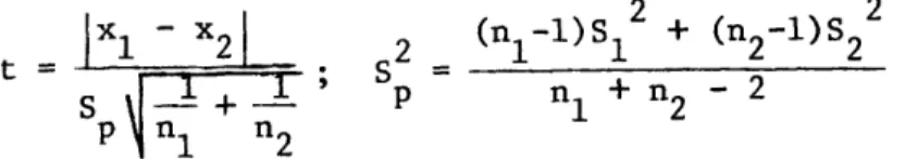
the ratios from each pair of sites. 4.3.1 Parametric Hypothesis Testing
One version of the Central Limit Theorem states that a collection of sample means from the same parent population distribution are normally distributed about the true population mean if each sample is sufficiently
large (n > 30). This property of sample means can be used to test the
hypothesis that two samples are taken from the same population distribution. If the sample means and variances are both equal at the same level of signifi-cance, the two samples can be assumed to be from the same population.