ParallelLCA: A foreground aware parallel calculator for
Life Cycle Assessment
by
François SAAB
THESIS PRESENTED TO ÉCOLE DE TECHNOLOGIE SUPÉRIEURE IN PARTIAL FULFILLMENT OF THE REQUIREMENTS FOR A MASTER’S DEGREE WITH THESIS IN SOFTWARE ENGINEERING
M.Sc.A.
MONTREAL, OCTOBER 25, 2019
ÉCOLE DE TECHNOLOGIE SUPÉRIEURE UNIVERSITÉ DU QUÉBEC
© Copyright reserved
It is forbidden to reproduce, save or share the content of this document either in whole or in parts. The reader who wishes to print or save this document on any media must first get the permission of the author.
BOARD OF EXAMINERS (THESIS M.SC.A.)
THIS THESIS HAS BEEN EVALUATED BY THE FOLLOWING BOARD OF EXAMINERS
Professor, Alain April, Thesis Supervisor
Department of Software Engineering and IT at École de technologie supérieure Professor Conrad Boton, President of the jury
Department of Construction Engineering at École de technologie supérieure Professor Mohamed Faten Zhani, Member of the jury
Department of Software Engineering and IT at École de technologie supérieure
THIS THESIS WAS PRESENTED AND DEFENDED
IN THE PRESENCE OF A BOARD OF EXAMINERS AND THE PUBLIC OCTOBER 17, 2019
ACKNOWLEDGMENTS
I would like first to thank Professor Alain April for his guidance concerning the academic writing of this thesis.
I also want to express my gratitude for the generous scholarship from the École Polytechnique de Montréal, which made it possible for me to pursue the Master’s program. Finally, I would like to thank the library staff at École de technologie supérieure for providing me with all the necessary advice and literature resources.
ParallelLCA: CALCULATEUR PARALLÈLE D’ANALYSE DE CYCLE DE VIE PRENANT COMPTE DE L’AVANT PLAN
François SAAB
RÉSUMÉ
L’analyse du cycle de vie (ACV), qui vise à évaluer les impacts environnementaux au cours du cycle de vie d’un produit (par exemple, la production d’aluminium au Québec) ou d’un système de produits, peut être utilisée pour comparer différents systèmes utilisant différents types de matériaux afin de déterminer celui qui est le moins dommageable pour l'environnement. Le calcul d’ACVreprésente un défi de calcul car il dépend de la taille du système de produit, du nombre d'itérations dans la simulation de Monte-Carlo, et du nombre de variables incertaines dans le système. Tout d'abord, la résolution d'un système linéaire, de dimensions dans l’ordre de 10 000 équations par 10 000 variables inconnues pour le cas de base. Deuxièmement, la construction d'un arbre, de nature itérative, avec des dimensions minimales de 10 000 nœuds. Troisièmement, la simulation de Monte-Carlo nécessitant plusieurs milliers d’itérations pour converger. Finalement, une analyse de sensibilité, qui nécessite le calcul des millions de corrélations vecteur-vecteur, dans laquelle chaque vecteur a une dimension qui est équivalente aux nombres des itérations qui sont effectués lors de la computation de Monte-Carlo.
Pour résoudre au mieux les défis informatiques présents dans l’ACV, la recherche bénéficie des bibliothèques standards pour la résolution de systèmes linéaires creux et du calcul sur des matrices creuses. En outre, la recherche a adoptée des optimisations mathématiques qui ont par exemple supprimé l’inverse matriciel de l’analyse de contribution qui est très coûteuse, ainsi que des optimisations algorithmiques qui ont pu enlever une grande partie d’analyse du calcul matriciel. De plus, la recherche a expérimenté avec des librairies, qui permettent de paralléliser le calcul, telles que OpenMP, MPI, et Apache Spark.
Dans un premier temps, ce mémoire abordera la littérature de ces opportunités de calcul. Deuxièmement, il présentera un calculateur d’ACVpour mettre en œuvre un calcul efficace. Enfin, il décrira les performances du calcul des différentes phases de l’ACV pour différentes dimensions du système (S) et se terminera par des suggestions d’améliorations et de développement futur.
Mots-clés: Analyse de Cycle de Vie (ACV), solveur hybride ACV, ACV parallèle, ACV distinguant l’avant plan
ParallelLCA: A FOREGROUND AWARE PARALLEL CALCULATOR FOR LIFE CYCLE ASSESSMENT
François SAAB
ABSTRACT
Life Cycle Assessment (LCA), which aims to assess the environmental impacts during the life cycle of a system product (S) (e.g., production of aluminum in Quebec), can be used to compare different systems built with different types of materials to determine which is the least harmful to the environment. The calculation in LCA represents a computational challenge as it is dependent on the size of the system, the number of iterations in the Monte-Carlo simulation, and the number of uncertain variables in the system. First, the solving of a linear system of dimensions in the order of 10,000 equations by 10,000 unknown variables is required for the base case. Second, the building of a graph iterative in nature with minimum dimensions of 10,000 vertices. Third, the computing of a Monte-Carlo simulation requiring several thousands of iterations to converge is to be computed. Finally, a sensitivity analysis which requires the computing of millions of correlations between vectors each having a dimension that is proportional to the number of iterations in the Monte-Carlo simulation. To best solve the computational challenges present in LCA, this research benefits from well-established libraries that solve large sparse linear systems and performs large sparse matrix computing. Also, this thesis adopted mathematical optimizations that removed the matrix inverse step from the contribution analysis module, which is very expensive, as well as other algorithmic optimizations that removed the large and variant part of the LCA supply-chain from the matrix component of the various calculation phases. Furthermore, this research experimented with libraries such as OpenMP, MPI, and Apache Spark to parallelize the computation.
First, the thesis will discuss the literature regarding these computational opportunities. Second, it will present a proposed LCA calculator for implementing an efficient LCA computation. Finally, it will present the performance of computing the different phases of LCA for various dimensions of the system (S) and concludes with suggestions for improvement and future development.
Keywords: Life cycle assessment (LCA), LCA Hybrid Solver, Parallel LCA, Foreground
TABLE OF CONTENTS
Page
INTRODUCTION ...1
CHAPTER 1 LITERATURE REVIEW ...6
1.1 Life cycle assessment algorithms ...6
1.1.1 Concepts and definitions ... 6
1.1.2 The Sequential Method for LCA ... 7
1.1.3 The Matrix Method for LCA ... 8
1.1.4 Uncertainties and Data Quality Indicators (DQI) in LCA databases ... 10
1.1.5 Sensitivity Analysis methods for LCA ... 13
1.1.6 Uncertainty propagation in LCA ... 15
1.1.6.1 Analytical uncertainty propagation for LCA ... 16
1.1.6.2 Sampling-based uncertainty propagation methods for LCA ... 17
1.1.7 Aggregated dataset uncertainty propagation for LCA ... 19
1.2 Parallel computing ...20
1.2.1 Parallel computing models ... 20
1.2.2 Bulk Synchronous Parallel (BSP) model ... 21
1.2.3 Parallelism levels and granularity ... 22
1.2.4 Parallel instructions stream ... 22
1.2.5 Architectures for parallel computing ... 23
1.2.6 The laws of parallelism ... 24
1.2.6.1 Amdahl’s Law: Fixed-size speedup ... 25
1.2.6.2 Gustafson’s Law: Scaled Speedup ... 26
1.2.7 OpenMP ... 27
1.2.7.1 Thread scheduling ... 27
1.2.7.2 Variables sharing ... 28
1.2.7.3 OpenMP Execution Constructs ... 28
1.2.7.4 OpenMP Synchronization Constructs ... 29
1.2.8 MPI ... 29
1.2.8.1 Communication groups ... 29
1.2.8.2 Communication primitives ... 30
1.2.8.3 BOOST::MPI ... 31
1.2.9 Apache Spark ... 32
1.2.9.1 RDD: Resilient Distributed Datasets ... 32
1.2.9.2 Execution model ... 33
1.2.9.3 RDD transformations and actions ... 33
1.3 Solving linear systems: General concepts and software libraries ...35
1.3.1 Linear systems solving concepts ... 35
1.3.2 Concepts and methods for solving sparse linear systems ... 37
1.3.3 Concepts and methods for computing the matrix inverse ... 40
1.3.4 Matrix computing libraries ... 41
1.4.1 Parallel framework review ... 46
1.4.2 Matrix libraries performance review ... 48
1.4.2.1 Direct solvers review ... 48
1.4.2.2 Iterative solvers review ... 49
1.4.2.3 Matrix inverse libraries review ... 51
1.4.3 LCA calculators review ... 53
1.5 Conclusion ...54
CHAPTER 2 PARALLEL FOREGROUND AWARE LCA ...56
2.1 Prototype Scope and Goals ...56
2.1.1 Research scope ... 56
2.1.2 Functional requirements ... 56
2.2 Calculator modules overview ...57
2.3 REST Service ...63
2.4 Parallel LCADB ...65
2.5 Calculator data loading ...69
2.6 Parameters module using EXPRTK ...70
2.7 Parallel LCA graph building using OpenMP ...72
2.8 Calculator Kernel ...78
2.8.1 Loading the Matrices: A, B, and Q and their indexes ... 78
2.8.2 LCA activities scalars computing ... 79
2.9 Foreground-Background LCA: Optimization for large systems ...79
2.10 Hybrid Algorithm for solving the Foreground-Background layers ...80
2.11 Matrix-based solving scripts ...83
2.11.1 Direct and iterative sparse system solving ... 83
2.11.2 Matrix inverse experimentation ... 84
2.12 LCI and LCIA vectors ...84
2.12.1 The Traditional Matrix Method ... 84
2.12.2 The Hybrid computing of LCI and LCIA ... 85
2.12.3 The Hybrid-Aggregation method ... 85
2.13 Aggregate upstream computation ...87
2.13.1 Aggregate upstream reformulation: matrix inverse avoidance and dimensionality reduction ... 87
2.13.2 Parallel aggregate upstream: MUMPS-MPI and Eigen++-OMP ... 89
2.14 Process contribution to LCI and LCIA ...90
2.15 Parallel LCIA upstream for multiple impact targets using OpenMP ...91
2.15.1 Computing cyclic upstream ... 92
2.15.1.1 Hybrid aggregate upstream ... 93
2.15.2 Cyclic to acyclic graph transformation ... 94
2.15.3 Acyclic upstream LCIA ... 96
2.16 Stochastic prototypes ...97
2.16.1 Main Features of the Prototypes ... 98
2.16.2 Prototypes for Parallel Monte-Carlo and Parallel GSA ... 101
2.17 Monte-Carlo sampling (MCS) and uncertainty propagation ...102
2.17.2 Pre-sampling MCS ... 104
2.18 SCC based GSA ...104
2.18.1 In-ranking SCC ... 104
2.18.2 Pre-ranking SCC ... 106
2.19 Aggregated datasets based MCS ...106
2.20 Conclusion ...110
CHAPTER 3 LIFE CYCLE ASSESSMENT ON APACHE SPARK...111
3.1 Apache Spark static LCA kernel implementation ...111
3.2 The validity of Apache Spark for LCA projects ...115
3.3 Conclusion ...119
CHAPTER 4 RESULTS AND DISCUSSION ...120
4.1 Results Validation - Comparison with OpenLCA and Brightway ...120
4.1.1 Use Case of “Aluminium Production in Quebec” from Ecoinvent 3.3 Database ... 120
4.1.1.1 Static phase validation with OpenLCA7 ... 120
4.1.1.2 Stochastic phase validation with Brightway2 ... 121
4.1.2 Use Case of Front layer Added to the Background Layer ... 122
4.1.2.1 Static phase validation for systems with foreground layer with OpenLCA7 ... 123
4.1.2.2 Stochastic LCA comparison of algorithm 2.8 and algorithm 2.5 ... 124
4.2 Calculator Performance Characteristics ...125
4.2.1 Simulation Setup, Benchmarking tools, and Graphics generation ... 125
4.2.2 Performance of the Calculator for Ecoinvent 3.3 Database ... 126
4.2.2.1 Parallel Graph Building ... 126
4.2.2.2 Static Phase ... 127
4.2.2.3 Stochastic Phase ... 128
4.2.3 Variant Size Performance Benchmark ... 135
4.2.3.1 Foreground generation Procedure ... 135
4.2.3.2 Pre-calculation phases ... 136 4.2.3.3 Static Phases... 137 4.2.3.4 Stochastic phases ... 140 4.3 Discussion ...141 4.3.1 Algorithms validation ... 143 4.3.1 Algorithms performance ... 144 4.4 Conclusion ...151 CONCLUSION 152 ANNEX I Simulation environment: Detailed CPU Information ...155
ANNEX II Calculator setup, code, and demos ...157
ANNEX IV Stochastic LCIA Raw Data ...163
ANNEX V Aggregated Scores Error ...169
ANNEX VI Matrix solving code samples ...171
ANNEX VII CSV Files and LCA model schemas ...172
ANNEX VIII LCAIndex schema...174 BIBLIOGRAPHY 175
LIST OF TABLES
Page
Table 1.1 Lognormal, normal, uniform, and triangular distributions ...11
Table 1.2 Pedigree Matrix, Version 2 ...12
Table 1.3 Pedigree Matrix, Variances ...13
Table 1.4 Flynn model for parallel computers ...23
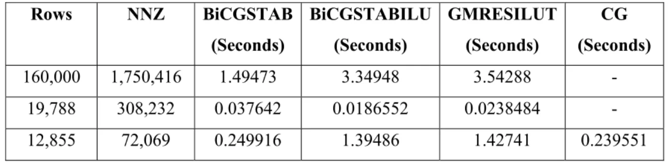
Table 1.5 Time of direct sparse solvers of the Eigen++ library. ...49
Table 1.6 Time of sparse iterative solvers in the Eigen++ library. ...50
Table 1.7 ViennaCL vs. PETSc time per solver iteration benchmark. ...50
Table 1.8 ViennaCL performance for large matrices. ...51
Table 1.9 MapReduce matrix inversion experiment setup. ...51
Table 1.10 Calculators—matrix computing libraries ...53
Table 1.11 Calculators—Monte-Carlo and GSA methods ...53
Table 1.12 Calculators—features comparison. ...54
Table 2.1 LCADB Store Structure ...67
Table 2.2 LCA Indexes Structure ...68
Table 2.3 Supported Uncertainties ...68
Table 4.1 Foreground examples ...123
Table 4.2 Test Servers Characteristics ...125
Table 4.3 Execution time for Monte-Carlo OpenMP of Figure 4.10 ...130
Table 4.4 Execution time for Monte-Carlo on OpenMP of Figure 4.12 ...132
Table 4.5 Execution time for pre-aggregated datasets Monte-Carlo ...133
Table 4.6 Phase performance for Ecoinvent 3.3 process. ...141
Table 4.7 Phases performance for Pre-calculated background layer. ...141
Table 4.9 Traditional A-1 scripts performance ...144 Table 4.10 Thesis QBA-1 solvers performance for Recipe Midpoint I ...144
LIST OF FIGURES
Page
Figure 1.1 Scalability, Efficiency, and Speedup ...25
Figure 1.2 Amdahl speedup vs. the number of cores. ...26
Figure 1.3 MPI Communication primitives ...30
Figure 1.4 Example of serialization for BOOST:: MPI. ...32
Figure 1.5 Krylov solving example ...39
Figure 1.6 Spark vs. MapReduce for K–Means ...46
Figure 1.7 MPI vs. Apache Spark for KNN...47
Figure 1.8 Matrix inverse on Spark vs MPI vs MapReduce. ...52
Figure 2.1 ParallelLCA calculator steps. ...58
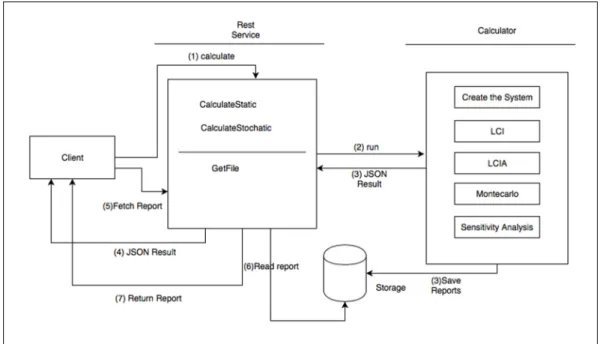
Figure 2.2 The REST service – ParallelLCA communication ...59
Figure 2.3 Calculator model architecture ...60
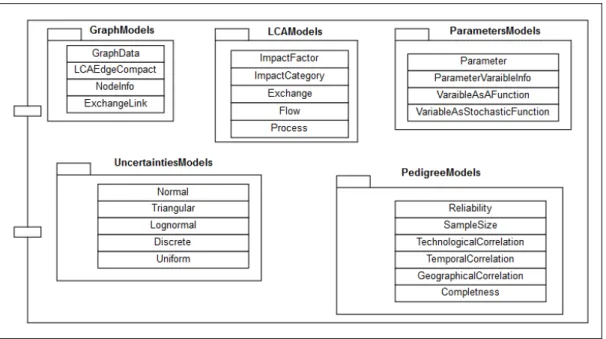
Figure 2.4 Calculator class models ...61
Figure 2.5 Object Factory models ...62
Figure 2.6 Utility functions ...62
Figure 2.7 Reporting module ...63
Figure 2.8 Program Flow ...64
Figure 2.9 Calculator Files Structure ...65
Figure 2.10 LCADB Differential Model ...65
Figure 2.11 Database Loading Workflow ...66
Figure 2.12 Loading LCADB using OpenMP ...67
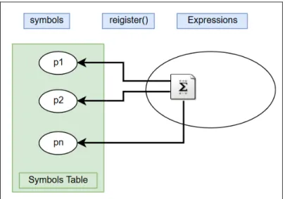
Figure 2.13 Symbols, expression, and symbols Table ...71
Figure 2.15 Layered Cyclic LCA Graph ...73
Figure 2.16 Graph building kernel ...74
Figure 2.17 Parallel iterative graph building using OpenMP ...74
Figure 2.18 Solving kernel on establishing a connection ...77
Figure 2.19 matrix A building ...78
Figure 2.20 Foreground-Background layers connection ...80
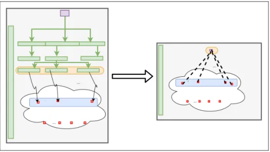
Figure 2.21 Foreground layer collapsing – equivalent LCA system ...81
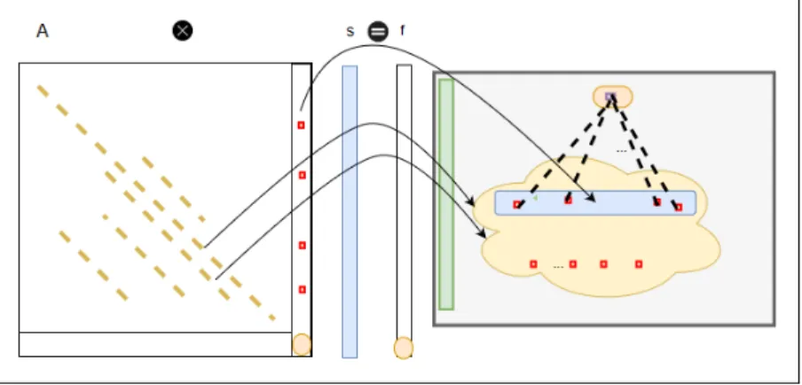
Figure 2.22 The new matrix A(Collapsed Foreground + Background Layer) ...82
Figure 2.23 Eigen++ BiCGSTAB solving implementation. ...83
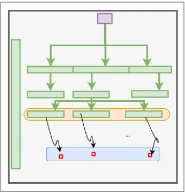
Figure 2.24 Aggregated background layer. ...85
Figure 2.25 Collapsed-Aggregated LCA system ...87
Figure 2.26 Aggregate LCIA Re-formulation. ...87
Figure 2.27 Upstream aggregation optimization. ...88
Figure 2.28 Parallelizing QBA-1 using OpenMP ...89
Figure 2.29 Cyclic LCA Graph ...92
Figure 2.30 Non-repetitive Acyclic Network ...94
Figure 2.31 Parallel upstream aggregated hierarchical graph ...97
Figure 2.32 Stochastic module architecture ...97
Figure 2.33 MCS input and output samples...98
Figure 2.34 2D Vectors exchanging in OpenMP/MPI ...99
Figure 2.35 Pre-sampling parallelism ...100
Figure 2.36 Pearson implementation – implicit vectorization ...106
Figure 2.37 Aggregated background layer graph model ...107
Figure 3.1 LCA Graph building on Apache Spark. ...112
Figure 3.2 Loading A in Apache Spark ...114
Figure 3.3 Loading B in Apache Spark ...115
Figure 3.4 Subset extraction ...117
Figure 4.1 Ratio of LCIA scores for ...121
Figure 4.2 Error in the uncertainty of Thesis calculator. ...122
Figure 4.3 Ratio of LCIA scores: OpenLCA7 vs. ParallelLCA Hybrid Solver ...123
Figure 4.4 Error in the LCIA scores for 6,000 iterations for ...124
Figure 4.5 Building (g) in Memory, serial vs. parallel versions ...126
Figure 4.6 Foundational LCA performance profile ...127
Figure 4.7 Contribution reports performance ...128
Figure 4.8 Execution time for serial Monte-Carlo of the activity production ...129
Figure 4.9 Stochastic LCA kernel performance profile ...129
Figure 4.10 Execution time for parallel Monte-Carlo using OpenMP. ...130
Figure 4.11 MPI vs. OpenMP for full MCS On the Leda server ...131
Figure 4.12 Monte-Carlo using OpenMP for a large number of iterations. ...132
Figure 4.13 Spearman ROCC vs iteration size ...134
Figure 4.14 Spearman ranking OpenMP on multicore ...134
Figure 4.15 Pre-calculation phases Time (seconds) for variant size foreground ...136
Figure 4.16 Performance for variant size foreground layer ...137
Figure 4.17 Other phases of the kernel solving using the Matrix Method ...138
Figure 4.18 Variant size foreground layer performance using the Hybrid Solver ...139
Figure 4.19 Variant size foreground layer influence on the performance ...139
Figure 4.21 Upstream report sub-sections ...145
Figure 4.22 Aggregate upstream subsections ...146
Figure 4.23 Scalability of Monte-Carlo OpenMP ...147
Figure 4.24 Speedup of Monte-Carlo OpenMP. ...148
LIST OF ALGORITHMS
Page
Algorithm 1.1 Monte-Carlo Sampling. ...18
Algorithm 2.1 Parallel and iterative graph building ...75
Algorithm 2.2 Hybrid solving algorithm. ...82
Algorithm 2.3 LCIA scores for the collapsed-aggregated system ...86
Algorithm 2.4 Upstream aggregate LCIA by reverse graph propagation ...93
Algorithm 2.5 Acyclic non-repetitive graph building ...95
Algorithm 2.6 Monte-Carlo proposed implementation ...103
Algorithm 2.7 SCC proposed algorithm ...105
Algorithm 2.8 Background layer scores aggregation ...108
LIST OF ABBREVIATIONS
ARPACK ARnoldi PACKage
Brightway2 Open Source LCA Software in Python
BLACS Basic Linear Algebra Communication Sub-programs BLAS Basic Linear Algebra Subprogram
CCDF Complementary Cumulative Density Function CDF Cumulative Density Function
CIRAIG Centre International de Reference sur Le Cycle de Vie des Produits CMLCA Scientific software for LCA, IOA, EIOA
COO Coordinate matrix
COLT Sparse matrix library developed by CERN CSC Compresses Sparse Column matrix
CSR Compressed Sparse Row matrix CuSPARSE Cuda Sparse library
Ecoinvent Proprietary life cycle inventory database EcoSpold Life cycle inventory database format Eigen++ C++ library for linear algebra
GSA Global Sensitivity Analysis GSL GNU Scientific Library
HPC High-Performance Computing
LCIA Life Cycle Impact Assessment
LCI Life-Cycle Inventory LU LU matrix decomposition
MCS Monte-Carlo Sampling
MD Multi Dissect matrix ordering
METIS Serial Graph Partitioning and Fill-Reducing matrix ordering MLlib Apache Spark's machine learning library
MTJ Matrix Toolkit for Java matrix library
MUMPS Multi-Frontal Un-Symmetric Matrices Parallel Solver NNZ Non-Zero entries in a matrix
OpenLCA Open Source LCA Software in Java OpenMP Open Multiprocessing
ParallelColt Parallel version of Colt a sparse linear algebra library in Java PDF Probability Density Function
QR QR matrix decomposition
RDD Apache Spark’s Resilient Distributed Datasets Revit Construction modelling software RNG Random Number Generator
Scalanlp library for natural language processing in Scala ScaLAPACK Fortran Library for scalable linear algebra package SCC Spearman Correlation Coefficient
SOR Successive Over-Relaxation
Apache Spark Library for distributed computing on massive datasets
SRS Software Requirement Specifications STDLIB The C++ standard library
SuperLU Library for linear algebra SVD Singular Value Decomposition UMFPACK Un-Symmetric Multifrontal Package
LIST OF SYMBOLS
1D One Dimensional
2D Two Dimensional
aij Cell in matrix A at row i and column j
A Technology matrix
bmn cell in matrix B at row m and column n
B Intervention Matrix
g Impact Score vector (g) LCA network or graph
h Inventory vector
P Parameters vector
p parameter in the parameters vector qkl cell in matrix Q at row k and column l
Q Characterization Matrix
INTRODUCTION
The use of products (e.g. the use of buildings or cars) exchanges materials with the environment either through extraction from nature (e.g., water and minerals) or through emissions into the air (e.g., CO2). Products that we use daily are created in factories by a chain of manufacturing processes (e.g., energy production, mining, and transport activities). This chain of processes extracts materials from nature, transforms those materials into complexes, and by doing this, generates pollutants that have various impacts in various areas of the environment (e.g., on human health, on climate change).
LCA (Life Cycle Assessment) is an established framework which aims at assessing the environmental impacts of a given product on the different areas in the environment by quantifying the impact of the life cycle of that product on the environment, highlighting impactful underlying industrial processes on a specific impact area. A series of iterative development phases in LCA has provided with LCA databases where industrial activities are represented as processes producing and consuming products through what is called intermediate exchanges. Also, each process exchanges elementary flows with the environment (e.g., CO2, water).
Research Context
A standard procedure is usually adopted to assess the impact of using a given product. This procedure can consist of:
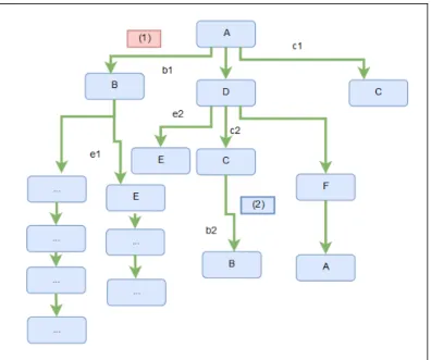
1. The building of a graph interconnecting the different LCA processes (i.e., Figure 0.1) based on the information provided in the adopted LCA database. This algorithm is iterative and requires database access in each iteration;
2. The traversing of the created graph, which may be cyclic, and the aggregating of the processes individual impact scores to assess the total impact. Alternatively, this step can be replaced by transforming the network into a system of linear equations which if solved
and scaled, can give the total impact scores of the involved activities. When the Matrix Method is used, additional matrix operations, namely matrix-matrix and matrix-vector multiplications, are necessary to replace the graph aggregation operation. This Calculation Kernel is the core of this research project;
3. The inverse of a matrix representing the created LCA graph is another type of expensive matrix operation to consider;
4. A Monte-Carlo simulation that requires several, tens, or hundreds of thousands of iterations to converge, wherein each iteration the aforementioned Calculation Kernel is executed;
5. A global sensitivity analysis which involves millions of vector-vector correlations to be computed. The central role of the sensitivity analysis is to identify significant contributors to the uncertainty of the output result.
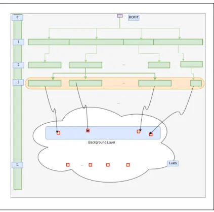
Figure 0.1 LCA Graph
Two kinds of processes interconnections are essential to distinguish in LCA: The background layer graph contains processes with cyclic interconnections, and the foreground layer (or front layer) graph consists of an acyclic graph of interconnections with mostly no Elementary
Flows exchanges. When modelling the lifecycle of “the use of a product” (e.g., phone or building) the different constituents of that product (e.g., screen, keyboard, electronics) are modelled as a hierarchical foreground graph that connects to processes from the background layer.
Research challenges
A primary goal in this research is the development of algorithms that provide scientifically correct results (e.g., similar to other standard LCA calculators). In addition to this functional requirement, other non-functional computational challenges make an essential constituent of this research, such as:
1. The efficient instant loading of a database that changes in content and increases in size to up to hundreds of thousands of elements in the foreground layer;
2. The fast computation of the LCA graph which can increase in size. Building the graph (g) is a challenging task because:
A. The exchanges database can become large enough which makes the queries execution inefficient;
B. The graph can be very deep (i.e., composed of thousands of layers) and therefore, the corresponding complexity will depend on the number of layers in the graph, the number of activities per layer, and the size of the exchanges database.
3. The implementation of a fast Calculation Kernel which consists of the traversal and transformation of the graph (g) into a set of matrices for performing the solving of a linear system (i.e., A x = b) as well as the fast computation of Matrix-Vector product operations which is essential in LCA equations;
4. The fast computation of a matrix inverse with dimensions proportional to the number of processes in the graph (g).
In addition to the aforementioned kernel calculation steps, this research is required to generate reports that provide insights allowing for the interpretation of the foundational LCA results such as:
1. The process-based contribution analysis reports, which allow assessing the contribution of each process to the totals of the inventory and environmental impact results;
2. The process-based upstream contribution analysis reports, which provides the contribution of each activity upstream chain to the total computed impact score vector. This report involves other expensive operations such as the computation of a matrix inverse and the translation of the cyclic graph into an acyclic one;
3. The fast and scalable implementation of a Monte-Carlo simulation consisting of several thousands of iterations. Each of those iterations consists of sampling a large number of objects (i.e., hundreds of thousands), and applying the aforementioned Calculation Kernel;
4. The fast and scalable implementation of a global sensitivity analysis (GSA) calculator, which involves the computation of millions of correlations, each involving vectors with dimensions starting from multiples of at least 1,000 elements.
Methods and thesis plan
The thesis considered two design decisions for solving these computational challenges. First, it experimented with parallel frameworks that support parallel data processing, parallel task execution, and parallel matrix computing. Second, the thesis adopted a myriad of mathematical and algorithmic optimizations to achieve faster response times.
The thesis presents, in Chapter 1, the literature review and focuses on topics such as computational LCA, parallel computing, and sparse matrix computing. In Chapter 2, the calculator prototype design and implementation decisions are presented. Finally, Chapter 4 describes the different conducted experiments and then concludes with an interpretation of these experiments results.
CHAPTER 1 LITERATURE REVIEW
This literature review aims at covering the background behind the different domains of this research project, which includes computational LCA, linear algebra, numerical matrix computing, efficient computing, parallel computing, and parallel computing frameworks. The literature review provides all the necessary background information that is used in the remainder of this thesis with a focus on the practical aspects (i.e., algorithms, programming methods, software frameworks) of the research.
1.1 Life cycle assessment algorithms 1.1.1 Concepts and definitions
LCA (Life Cycle Assessment) is a systemic framework to assess the environmental footprint, from cradle to grave, of the life cycle of a product, which includes the raw material acquisition, the product manufacturing, the distribution, the use of the product, and the final disposal. The lifecycle of a product can be modelled as a Network (or a Graph) of connected processes. A Process, also called activity, is a step in the life cycle of a product (e.g., material extraction activity during electricity production). Intermediate Flows are the interconnections between the different processes of the lifecycle of a product (e.g., electricity production process connection to the process of crude oil). The interactions between an LCA process and its surrounding Biosphere are called Elementary Flows (e.g., extracting or emitting substances into nature, like CO2). An Inventory contains the total quantities of Elementary Flow exchanges with nature. Impacts on the environment are classified in corresponding Impact Categories, based on the concerned damaged area (e.g., water, air, human life), The step of converting the elementary flows inventory into impact categories scores is called Characterization. This step uses a list of Impact Factors which map each
elementary flow inventory into an impact score in a given impact category. Impact Methods represent, in LCA databases, a higher container for Impact Categories. Each impact method is responsible for several impact categories (ISO, 2006).
LCA consists of four phases. First, in the scope and definition phase, a Functional Unit, which is the definition of the function (or functions in the case of multi-functional LCA) provided by a product life cycle, is established. Second, in the inventory phase or LCI (Life Cycle Inventory), the totals of the different emissions and extractions with the environment (i.e., Elementary Flows) are quantified: each elementary flow exchange is assigned a total quantity. Third, in the impact assessment phase or LCIA (Life Cycle Impact Assessment), the inventories (e.g., 1 kg of wood), are characterized into respective impact categories and impact methods using the corresponding Impact Factors. Finally, in the interpretation phase, the framework assesses the contribution of each of the activities in the life cycle of a product to the total impacts and the total inventory results. Also, the interpretation phase may assess the uncertainty of the output results through what is called Uncertainty Propagation analysis. Following the uncertainty propagation analysis is a sensitivity analysis that can be performed to assess the effect of uncertainty in input parameters on the uncertainty in output results (ISO, 2006).
1.1.2 The Sequential Method for LCA
Jolliet, Soucy, and Houillon (2010) explained that a typical LCA calculation method, also called the Sequential Method, follows a series of steps for evaluating the inventory and the environmental impacts of a product lifecycle. It starts by identifying the Functional Unit (e.g., production of 1 kg diesel) of the system to analyze. It then identifies the demand-supply interconnections and scales the included processes to meet the requirement of the functional unit. The scaling of the processes scalars consists of propagating the Functional Unit from the root process in the downstream direction until reaching the leaf nodes or non-demanding processes.
After scaling the processes, the inventory is calculated as in equation 1.1 and characterized into Impact Categories using their Impact Factor coefficients as in equation 1.2.
𝐿𝐶𝐼 , the inventory of an elementary flow f is computed as an aggregation, as given by equation 1.1, over the array of all the LCA processes that exchange that flow with the environment.
𝐿𝐶𝐼 = 𝑠𝑐𝑎𝑙𝑎𝑟 ∗ 𝑈𝑛𝑖𝑡𝑎𝑟𝑦 𝑞𝑢𝑎𝑛𝑡𝑖𝑡𝑦 (1.1)
𝐿𝐶𝐼𝐴 , the impact score of an impact category c can be computed as an aggregation, as given by equation 1.2, over the inventory vector previously obtained from equation 1.1.
𝐿𝐶𝐼𝐴 = 𝐿𝐶𝐼 ∗ 𝐼𝑚𝑝𝑎𝑐𝑡 𝐹𝑎𝑐𝑡𝑜𝑟,
,
(1.2)
A significant challenge when using the Sequential Method is the possible presence of feedback loops (i.e., circular connections) in the network interconnecting the different LCA processes of the background layer. Those circular connections will cause the traversal of the graph never to finish. Several solutions to this problem have been proposed, such as:
“Interrupting a branch after a specified number of loops, interrupting a branch when the last round has added less than a specified amount, replacing process data by corrected process data in which feedback loops have been accounted for, and the use of infinite geometrical progression.” (Heijungs and Sun, 2002)
1.1.3 The Matrix Method for LCA
The Matrix Method, first introduced by Heijungs (1994) and further developed in Heijungs and Sun (2002), came to propose a new structure for computational LCA. This new structure
consists of converting the graph traversal and aggregations of equations 1.1 and 1.2 into matrix operations. In the following section, the thesis presents the main components of the Matrix Method and its internal operations.
Matrix A, the Technology Matrix, contains the unitary quantities of the intermediate exchanges (i.e., rows) associated with the LCA processes (i.e., columns) of a product lifecycle. Matrix B, the Biosphere Matrix, contains the unitary quantities of the elementary flows (i.e., rows) associated with the LCA processes (i.e., columns) of a product lifecycle. Matrix Q, the Impact Factors, has in its rows the Elementary Flows and in its columns the Impact Categories. Vector f, the Demand Vector, has all its cells set to zeros except one cell set to the functional unit quantity.
Vector s, the Scalars Vector, results from scaling the intermediate exchanges (i.e., rows in A) to produce the desired demand vector f. The scalars vector s can be computed using equation 1.3.
𝐴 𝑠 = 𝑓 , 𝑠 = 𝐴 𝑓 (1.3)
Vector g, the inventory vector, contains the total inventories of the elementary flows generated or extracted by a given product, and it is computed as in equation 1.4.
𝑔 = 𝐵 𝑠 = 𝐵 𝐴 (1.4)
Vector h, the Impact Scores vector, contains the total impacts of the impact categories belonging to the impact method understudy, and it is computed as in equation 1.5.
An important variable in matrix-based LCA is the inverse of the Technology Matrix A. Su and Heijungs (2007) provided the development of the matrix inverse method in LCA using power series expansion, as shown in equation 1.6.
𝐴 = 𝐼 𝐼 − 𝐴 𝐼 − 𝐴 𝐼 − 𝐴 ⋯
= 1 𝑍 𝑍 𝑍 ⋯
(1.6)
The individual column cells in A-1 represent the total output that each unitary process (i.e.,
matrix cells), in that given column, must produce to satisfy the reference flow of the process associated with the same column in A.
The process-based contribution to the total inventory of producing one unit of a given process P is given by first computing equation 1.7 and then selecting the column, in the resulting matrix, which position is equal to the position of process P in the original matrix A.
𝐿𝐶𝐼 = 𝐵 𝐴 (1.7)
Similarly, the process-based contribution to the total environmental impact of producing one unit of a given process P is given by first computing equation 1.8 and then selecting the column in the resulting matrix which position is equal to the position of process P in matrix
A.
𝐿𝐶𝐼𝐴 = 𝑄 𝐵 𝐴 (1.8)
1.1.4 Uncertainties and Data Quality Indicators (DQI) in LCA databases
We begin our exploration of uncertainties by listing some related definitions: 1. A population is a domain from which one observation is sampled;
observation from the possible domain of observations to a probability value;
3. Uncertainty can be caused by either a Random Variation or a Bias. A Random Variation corresponds to the randomness in the values of a given variable. A Bias is a skewness that was introduced to the observation because of a systemic measurement error.
Table 1.1 Lognormal, normal, uniform, and triangular distributions 𝑓(𝑥) = 1 𝑥 𝜎 √2 𝜋 𝑒 ( ( ) ) 𝑓(𝑥) = 1 𝑥 𝜎 √2 𝜋 𝑒 ( ( ) ) 𝑓(𝑥) = 1 ( 𝐵 − 𝐴 ) 𝑓(𝑥) = ⎩ ⎪ ⎨ ⎪ ⎧ 2(𝑥 − 𝐴) (𝐵 − 𝐴)(𝐶 − 𝐴) 𝑓𝑜𝑟𝐴 ≤ 𝑥 ≤ 𝐶 2(𝐵 − 𝑥) (𝐵 − 𝐴)(𝐵 − 𝐶) 𝑓𝑜𝑟𝐶 ≤ 𝑥 ≤ 𝐵 0 𝑒𝑙𝑠𝑒𝑤ℎ𝑒𝑟𝑒
Several statistical measures are to be considered when assessing uncertainties. The arithmetic mean is the sum of observation values divided by the count of the observations. The error is the deviation of an observation from the mean of its population. The variance is the sum of the squares of the error divided by the population size. The standard deviation is the root square of the variance. The median is the value that splits the population distribution in half. The mode is the most likely occurred observation. A two-sided confidence interval (e.g., 95%) is the central part of the distribution that is obtained by excluding a certain percentage (e.g., 2.5%) from both sides of the distribution.
Current LCA databases use four principal statistical distributions: the uniform, the triangular, the normal, and the lognormal distributions. These distributions are represented in different forms. The mathematical representation will give a formula for the PDF as in Table 1.1. The EcoSpold format provides the following fields for each of the uncertainty types: UncertaintyType, mean value, minValue, maxValue, most likely value, and standardDeviation95. The representation in the EcoSpold format is what is widely used in
current LCA databases.
In addition to the basic uncertainties, current LCA databases such as Ecoinvent provide Data Quality Indicators (DQI) that allows for the fine-tuning of the basic uncertainty to provide a more reliable PDF. Based on the provided DQI, additional uncertainties can be added to the lognormal representation of the initial PDF to provide with a Pedigree transformed PDF.
Table 1.2 Pedigree Matrix, Version 2 Taken from Mutel (2013)
Indicators Ranks (𝒖𝒊) 1 2 3 4 5 Reliability 1 1.54 1.61 1.69 1.69 Completeness 1 1.03 1.04 1.08 1.08 Temporal Correlation 1 1.03 1.1 1.19 1.29 Geographical Correlation 1 1.04 1.08 1.11 1.11
Further Technological Correlation 1 1.18 1.65 1.08 2.8
The Data Quality Indicators (DQI) are computed based on a ranking system that involves the use of expert domain judges. The Expert judges assess data sources with uncertainties according to five independent characteristics as listed in Table 1.2. Each of the characteristics is ranked, in a system of five quality levels, with a score between one and five. After the DQI scores are attributed based on a given uncertainty source information, a normal uncertainty distribution is computed for each of the DQI characteristics. Each of these distributions has a mean value of zero, and a variance as shown in Table 1.3. The uncertainty of the given source is then computed, as shown in equation 1.9. (Weidema et al., 2013)
Table 1.3 Pedigree Matrix, Variances Taken from Weidema et al. (2013)
Indicators Variances (𝒖𝒊) 1 2 3 4 5 Reliability 0 0.0006 0.002 0.008 0.04 Completeness 10 0.0001 0.0006 0.002 0.008 Temporal Correlation 10 0.0002 0.002 0.008 0.04 Geographical Correlation 0 2.5 10-5 0.0001 0.0006 0.002
Further Technological Correlation 0 0.0006 0.008 0.04 0.12
In addition to the pedigree for lognormal distributions, Muller et al. (2016a) provided equations and a procedure to compute the additional variances for distributions other than the lognormal.
1.1.5 Sensitivity Analysis methods for LCA
As explained by Groen, Bokkers, Heijungs, and de Boer (2017), several methods are commonly used for performing sensitivity analysis in LCA. We focus on the exploration of the sampling-based and correlation-based methods as they are part of the functional requirements for this research project.
For the Correlation-Based methods, the literature distinguishes two methods, among others: the Pearson Correlation Coefficient and the Spearman rank-order correlation coefficient. The Pearson Correlation Coefficient provides the correlation between two sample vectors 𝑝 and 𝑔 as in equation 1.10 below.
𝑟 = ∑(𝑝 − 𝑝) 𝑔 − 𝑔 ∑(𝑝 − 𝑝) ∑ 𝑔 − 𝑔
An alternative to the Pearson correlation coefficient method is the Spearman rank-order correlation coefficient (SCC) method, which measures the linear dependence between variables 𝑝 and 𝑔 . To compute the ranked correlation coefficient, the variables pi and 𝑔 are
replaced by their respective ranked vectors. Equation 1.11 applied to the ranked vectors gives 𝑟 . The sensitivity index, using this method, would be computed as in equation 1.12.
𝑆 = 𝑟 (1.11)
For the Variance-based methods, the Sobol method relies on calculating two main indexes, the Sobol Main Effect, and the Sobol Total Effect. The Sobol algorithm in LCA consists of repeating a sampling of three matrices in several iterations followed by the computation of output variable g or h to finally calculate the indexes in equation 1.12 and equation 1.13. The sampling step consists of first generating a matrix P containing the values of all input parameters pij. A second matrix Q is generated in the same way. Finally, for each column
from Q a third matrix R is generated by adopting that column from Q, and all other columns from P. Following this sampling, the output variables g or h are computed for each selection of a column from Q and for several iterations. The Sobol Main Effect 𝑆 , equation 1.12, measures the influence, on the output variable g or h, of the event of “fixing the parameter pij
and making all other parameters variant”. The Sobol Total Effect 𝑆 , equation 1.13, measures the influence on the output variable g of the event of “making all parameters fixed but parameter pij variable”.
𝑆 = 𝑣𝑎𝑟 𝐸 𝑔 𝑝 𝑉𝑎𝑟(𝑔) = 1 𝑁 ∑ 𝑔(𝑄) 𝑔 𝑅 − 𝑔(𝑃) 1 𝑁 ∑ {𝑔(𝑃) − (𝑁 ∑ 𝑔(𝑃) }1 (1.12) 𝑆 = 1 2𝑁 ∑ 𝑔(𝑝) − 𝑔 𝑅 1 𝑁 ∑ (𝑔(𝑃) ) − 𝑁 ∑ (𝑔(𝑃)1 (1.13)
Other methods that are available are based on the linear regression formulation and First Order-Taylor expansion.
According to the theory of multiple linear regression, the output g can be expressed as in equation 1.14. The coefficients 𝑐 , 𝑐 , and 𝑒 are the intercept, the slope, and the error terms respectively. The sensitivity index of g would be as in equation 1.15.
𝑔 = 𝑐 + 𝑐 𝑝 + 𝑒 (1.14)
𝑆 =𝑉𝑎𝑟 𝑝
𝑉𝑎𝑟(𝑔) 𝐶
(1.15)
Finally, for the Key-issue analysis methods, a commonly used method is the First-order Taylor expansion. Applying this method to LCA will give an expression of the output variable g using Taylor expansion as in equation 1.16. Using Taylor expansion, the sensitivity index would be calculated as in equation 1.17:
𝑔 = 𝑔 𝑃 = 𝑔 𝑝 +𝜕 𝑔 𝑝 𝜕 𝑝 𝑝 − 𝑝 (1.16) 𝑆 = 𝑉𝑎𝑟 𝑝 𝑉𝑎𝑟(𝑔) 𝜕𝑔 𝜕𝑝 (1.17)
1.1.6 Uncertainty propagation in LCA
A system can be modelled as a function Y of independent variables ( 𝑥 , 𝑥 , . . . , 𝑥 ). If there is uncertainty in the independent variables 𝑥, two main points of concerns are raised. A first
question is concerning the amount of uncertainty that is induced in the output variable because of the uncertainty in the input variables. This first question implies another equally
important question, which is how to propagate the uncertainty from input variables to output variables in order to assess the output uncertainty. A second question concerns the contribution of the uncertainty of a given input variable 𝑋 to the total uncertainty of the output variable Y. This section discusses the literature concerning these questions.
1.1.6.1 Analytical uncertainty propagation for LCA
The analytical approach of uncertainty propagation consists of treating the system as a function of input variables and applying differential calculus to propagate the uncertainty. Supposing Z is a function of variables x and y that represent the system; then, as explained in Heijungs and Sun (2002), the variance of Z is calculated as in equation 1.18.
𝑉 ≈ 𝜕 𝜕𝑥 . 𝑉 + 𝜕 𝜕𝑦 . 𝑉 + 2 𝜕 𝜕 𝜕 𝜕 𝐶𝑂𝑉 (𝑥, 𝑦) (1.18)
In the case where Z is dependent on more than two inputs, and if we ignore the correlation between the input variables, the variance is calculated as in equation 1.19 as a sum of the product of the Sensitivity Coefficient SC (equation 1.20) of a given parameter and the variance of that parameter.
𝑌 = 𝑓( 𝑋 , … , 𝑋 ), 𝑉(𝑌) ≈ 𝑆𝐶 . 𝑉 (𝑋 ) (1.19) 𝑆𝐶 = ∆ ∆ ≈ 𝜕 𝜕 (1.20)
As explained by MacLeod, Fraser, and Mackay (2002), for the particular case of input variables with lognormal distributions, which is very common in the sciences and LCA databases, the propagation of uncertainty can be approximated as in equation 1.21. The quantity GSD2 is the Confidence Factor (CF) characterizing a 95% confidence interval of the
variables x and y. Sx,h is the sensitivity of parameter x relative to the output result h and is computed as in equation 1.22. (𝑙𝑛 𝐺𝑆𝐷 ) = 𝑆 , (ln 𝐺𝑆𝐷 ) (1.21) 𝑆 , = 𝜕ℎ 𝜕𝑥 𝑥 ℎ (1.22) 𝐾 , = 𝑆 , ln 𝐺𝑆𝐷 ln 𝐺𝑆𝐷 (1.23)
The contribution of the uncertainty in the input variable x (i.e., GSD ) to the uncertainty in the output variable y (i.e., ln 𝐺𝑆𝐷 ) is given by equation 1.23.
1.1.6.2 Sampling-based uncertainty propagation methods for LCA
As explained by E. A. Groen, Heijungs, Bokkers and de Boer (2014) and by Peters (2007a),
Monte-Carlo sampling (MCS), a widespread sampling method, will first define a
compuTable format of the uncertainties in input parameters as PDFs (Probability Density Function). Second, MCS will proceed to the generation of pseudo-random samples for the uncertain cells in 𝐴 , 𝐵 , and 𝑄 based on their PDF definitions. Third, it will use the generated samples in equations 1.3, 1.4, and 1.5 to propagate the uncertainty from input parameters to the output result.
Algorithm 1.1 Monte-Carlo Sampling. Based on (Peters, 2007a)
Latin Hypercube Sampling (LHS) is a variant of the MCS, which employs a stratified
sampling approach instead of pseudo-random sampling one. In random sampling, random numbers are picked independently and at random for the different independent variables Xi.
As explained in Helton and Davis (2002), LHS will first identify the range of each variable and then divide that range into n LHS intervals with equal probability. Second, an array of random variables is generated with values are computed by randomly sampling one variable from each LHS interval. This process is repeated to select another N values for the independent variable Xi+1, and so on. The N values of Xi are paired at random and without
replacement with the values of Xi+1 to create LHS pairs of two variables. This array of pairs
will then be combined with the LHS values of a third variable Xi+2 to form a triplet of LHS
values. The process will be repeated for all uncertain independent variables. (Helton and Davis, 2002).
Quasi MCS (QMCS) is another variant of MCS with the difference of not using the default
the random number sampling. QMCS uses quasi-random numbers to sample from the distribution functions. As shown in Saltelli et al. (2007), MCS pseudo-number generated samples tend to have clusters and gaps. When using independent variables with Clusters, functions that exist in the vicinity of that cluster are overemphasized in statistical analysis. On the other hand, when independent variables have gaps, the function values that are
dependent on these variables will not be sampled. Quasi-random generators produce sequences having the property of near uniformity, where clusters and gaps are eliminated. The process of generating quasi-random numbers consist of generating deterministic sequences of numbers taking into consideration the position of previously sampled points (Tarantola, Becker and Zeitz, 2012).
1.1.7 Aggregated dataset uncertainty propagation for LCA
In a study published by Qin and Suh (2017), unitary process-level exchanges PDFs were sampled. This sampling was repeated 1,000 times for all of the exchanges of each process independently. For each process, 1,000 samples of 1,000 exchanges were selected, which sums up to a million samples per process. This study tries to find the distribution that best fits aggregate LCI at the level of each unitary LCA process. In finding the best fit, the research is trying to find an approximate PDF to represent the unitary processes aggregate LCI. This study found that most of the aggregate LCIs in the Ecoinvent 3.1 database follow a lognormal distribution. Consequently, the study suggested that using lognormal PDF approximations of aggregated LCI, the sampling is only needed on the approximate PDFs and that evaluating the detailed supply-chain of each process can be avoided.
In a reply letter to Qin and Suh (2017) paper, Heijungs, Henriksson and Guinée (2017)) reasoned that in a comparative LCA, uncertainty has to be deduced from samples generated dependently and that using pre-calculated distributions of complete systems generated from samples that are generated independently will lead to a large overestimation when assessing the uncertainty of the final output results.
Qin and Suh (2017) re-visited their study and re-published a related paper. In this revision and according to empirical results, they show that the use of pre-calculated LCIs “leads to a slight underestimation rather than an overestimation.” Furthermore, they considered that the error in the GSDs of the LCI arrays generated from either pre-calculated LCIs or full MCS is
negligible and that “in practice, pre-calculated LCIs can be used in understanding the uncertainties of both non-comparative and comparative LCA.”
Finally, Lesage et al. (2018) conducted a study comparing the results of using pre-calculated aggregated LCI when using independent and dependent sampling. The research concluded that “independent sampling should not be used for comparative LCA” and that dependently pre-sampled and aggregated LCIs provides quick and correct results. The method of Lesage et al. (2018) consists of first sampling the uncertain cells dependently, second iterating over all the Ecoinvent activities and calculating the quantities g and h. Finally, it saves the results as 2D arrays. The researchers in this paper argue that while this method provides results with a minimal error when compared to full MCS, it also allows performing Monte-Carlo without re-evaluating the Ecoinvent background layer activities, and solving the corresponding linear system for each MCS iteration as it is the case of full MCS shown in algorithm 1.1.
1.2 Parallel computing
Parallel computing provides a set of models, architectures, and frameworks to achieve parallel processing at the data and task levels. This section will present the models and architectures behind parallel computing. In addition, in this section, we will provide a background review of three widely used parallel frameworks: MPI, OpenMP, and Apache Spark. This review will begin by exploring the basic concepts in parallel computing, and then it will switch the focus to more practical programming-oriented aspects which are heavily used in this research project.
1.2.1 Parallel computing models
The Fork-Join model, implemented in POSIX (Nichols, Buttlar and Farrell, 2013) and OpenMP (Chapman, Jost and Pas, 2008) among others, is a model composed of two phases: fork and join. In the fork phase, the work is initially divided into smaller tasks that can be
computed independently and therefore executed in parallel. In the join phase, using a synchronization point, results of the parallel tasks are reduced or joined into one result. The Message Passing Model, implemented in MPI (Geist et al., 1996) for example, is a model where each processor uses a private memory to store its variables, which cannot be accessed by other processors. A processor can exchange messages with other processors using inter-process communication. The two main primitives for messages exchanging are Send and Receive, which can be done either synchronously or asynchronously.
The Data flow model, implemented for instance, in Apache Spark (Zaharia et al., 2016), transforms the program tasks into a graph of dependent and independent tasks. Dependent tasks must be executed sequentially (i.e., one at a time) and independent tasks can take advantage of parallel.
1.2.2 Bulk Synchronous Parallel (BSP) model
Bulk Synchronous Parallel (BSP) is an abstract model that was introduced in (Valiant, 1990) to find a hardware-software bridge for the parallel programs similar to what the Von-Neuman model provided for sequential programs. BSP allows for the design of parallel algorithms by dividing the program to compute in several super-steps (i.e., iterations in an iterative program). Each super-step will follow a protocol defined by BSP. First, in the concurrent computation step, components of the computation are allowed to run locally in parallel. Second, in the communication step, processes exchange messages through routers and share data using various communication primitives. Third, in the synchronization barrier step, processes cannot proceed before all processes have reached the barrier. The synchronization step can happen for each period L, also called the Periodicity Parameter.
1.2.3 Parallelism levels and granularity
There are three primary levels of parallelism. The Instruction Level Parallelism (ILP), is where instructions are executed on a Vector of data in parallel in the CPU registers. Instruction level parallelism must be enabled at the hardware level through the availability of CPU architectures, and code compilers need to generate explicit vectorized code that can run on such hardware architectures (e.g., matrix-matrix multiplication). The Data Level Parallelism (DLP) is found in applications where a large amount of data is available, the data is split into chunks, and a single processor works only on a single chunk instead of the whole dataset (e.g., massive datasets queries). Finally, Task Level Parallelism (TLP) is adopted when different tasks need to be run in parallel by different processors on different streams of data (multi-processing programming using MPI).
Also, parallelism can be applied at different frequencies. In Fine-grained parallelism, the data transfers are frequent and occur at the instruction level between the involved processors. In Mid-grained parallelism, data transfer is less frequent and occurs at a higher level between the program sub-tasks. In Coarse-grained parallelism, data transfers only occur when parallel processors finish their work and want to join the individual results into a final result.
1.2.4 Parallel instructions stream
The execution model of a sequential computer is based on the Von Neumann machine (Von Neumann, 1993) and is characterized by a single instructions stream in which one instruction is applied on a single data item. However, in parallel computing, a program at the low-level physical layer consists of one or many instruction streams acting on one or many data streams.
Table 1.4 Flynn model for parallel computers Taken from Flynn (1972)
Instruction / Data
Single Multiple Single SISD (e.g., uniprocessor or
sequential computers)
MISD (e.g. systolic arrays) Multiple SIMD (e.g., vector and
data-parallel architectures)
MIMD (Multi-processes running each on its own data stream)
Flynn (1972) introduced four architectures for parallelism based on how instructions are being applied on data streams, as shown in Table 1.4. These architectures can be described as follows:
• SISD (Single Instruction Single Data): this type of architecture is widespread in traditional CPUs where each instruction is executed on a single stream of data;
• SIMD (Single Instruction Multiple Data): this type of architecture is what operates vector computers, for example. In this type of computers, multiple processors are executing the same instruction on data items spread across multiple CPUs;
• MISD (Multiple Instruction Single Data): implemented in systolic arrays (Kung & Leiserson, 1978);
• MIMD (Multiple Instruction Multiple Data): in this model of computers, different datasets are spread across multiple CPUs where each executes its own stream of instructions.
1.2.5 Architectures for parallel computing
The literature distinguishes between two types of parallel computer architectures: Symmetric Shared-memory multiprocessor (SMP) and Distributed Memory Architecture (Nielsen, 2016).
SMP architecture considers all cores as independent computing units sharing the same memory. The various types of shared memory being used influence the performance in this model. The following are the different types of memory types from fastest to slowest: 1) processors register memory 2) L1, L2, L3 cache memories, 3) hard-disk drives, and 4) remote disks on a network.
Distributed Memory Architecture is a model where each process stores its variables in a private memory that is not accessible to other processors. Data can be shared only by exchanging messages between processors, and therefore, the network communication properties such as Latency, Bandwidth, and Topology are the most influencers in this model. Latency is the time to initiate message passing. Bandwidth is the rate of exchanging messages. Topology is how the different processes are interconnected (i.e., star, grid, etc.).
1.2.6 The laws of parallelism
Let Tseq denote the time for running a program serially, TP the time taken to run an equivalent parallel program using P processors, and T1 the execution time of that parallel version using a single processor. Three useful metrics are essential to measuring the performance of a proposed parallel algorithm: 1) Scalability, 2) Speedup, and 3) Efficiency.
Scalability is the ratio between the computation time when running on P’ processors versus the computation time when running on P processors where P’< P. This metric gives insights on how the performance changes when adding one processor at a time to the pool of resources running a given program.
The speedup is the ratio between the execution time of scenario “B” consisting of running the same parallel version on a single processor denoted by t1, and the execution time of scenario “A” consisting of running a given parallel version of a program on P processor denoted by tp. Speedup increases with the addition of new processing units only when tp continue in decreasing.
Figure 1.1 Scalability, Efficiency, and Speedup
Efficiency is the ratio of the Speedup when using P processors over the number of processors P. This number provides an insight on the efficiency of adding more cores to the simulation. Usually, efficiency drops when adding more parallelism due to the overhead of parallelism caused by threads synchronization or processors communication.
1.2.6.1 Amdahl’s Law: Fixed-size speedup
The time to run a program in parallel can be modelled as consisting of two portions, a parallel portion denoted by 𝛼 and sequential portion denoted by s. This model is characterized by 𝛼 + 𝑠 = 1. The speedup for this model, as described by the Amdahl law, is calculated as in equation 1.24 (Amdahl, 1967).
𝑆𝑝𝑒𝑒𝑑𝑢𝑝(𝑃) = 1 𝑠 + 𝛼 𝑃
(1.24)
Based on this law, the speedup is upper bounded by αseq (i.e., the non-parallelizable code) as in equation 1.25. Hence, the speedup is highly dependent on the sequential part of the program.
Lim
→ 𝑆𝑝𝑒𝑒𝑑𝑢𝑝(𝑃) =
1 𝛼
(1.25)
Figure 1.2 Amdahl speedup vs. the number of cores. Based on equation 1.24
1.2.6.2 Gustafson’s Law: Scaled Speedup
Gustafson re-evaluated Amdahl’s law by studying the influence of increasing both the number of processors P and the size of data or tasks n being processed by the P processors. This revaluation introduced a new speedup called the scaled speedup, as presented in equation 1.26 (Gustafson, 1988).
𝑆𝑝𝑒𝑒𝑑𝑢𝑝 (𝑃) = 𝛼 + 𝑃 𝛼 (1.26)
The scaled speedup studies practical situations where the software application uses more computing resources when the size of data or tasks increases.
Lim
→ 𝑆𝑝𝑒𝑒𝑑𝑢𝑝 (𝑃) = 𝑃 𝛼 (1.27)
1.2.7 OpenMP
OpenMP (Dagum and Menon, 1998), is a well-known standard in shared memory parallel programming which promotes code annotations (i.e., compiler directives) that is translated by specialized compilers into parallel code. OpenMP provides the user with compiler directives to configure thread scheduling, to specify parallel and synchronization regions, and to define variables scope (e.g., shared or private).
1.2.7.1 Thread scheduling
OpenMP allows defining parallel regions with one of the pre-configured types of scheduling. As explained in Chapman et al. (2008), when the first parallel region is encountered, the master and workers thread is created, and the work is split among the different threads based on the preconfigured type of scheduler. When a parallel region execution is finished, the worker threads switch to Sleep mode, and the Master thread remains active. When the next parallel region is encountered, the idle worker's threads are reused instead of created as new threads.
The most common scheduling types can take on the following values:
o Static: In this scheduling type, OpenMP divides the work into chunks of size chunk-size (i.e., given as a parameter), and schedules the execution of these chunks by the available threads in a circular order;
o Dynamic: In this scheduling mode, OpenMP splits the work into chunks of size chunk-size, and each thread executes a chunk of the work and then requests additional chunks until the work is done;
o Guided: In this scheduling mode, which is similar to the dynamic mode, the chunk size is controlled by the OpenMP framework for better load balancing;
o Auto: In the auto-scheduling type, OpenMP delegates the decision of the scheduling
mode to the compiler or the runtime system;
o Runtime: In the runtime scheduling type, OpenMP defers the decision about the
scheduling until runtime.
1.2.7.2 Variables sharing
OpenMP allows for the creation of variables as private to individual threads or as shared among threads. The following is a list of supported variables scopes:
o private: A variable is considered as private if it is initialized and owned by one of the OpenMP threads. Each thread can do its modification to its own private variables without the requirement to synchronize with other threads. Private variables cannot be accessed from outside of the OpenMP context;
o firstprivate: Similar to private variables, firstprivate variables get their values initialized when copied from the master thread to the inside of an OpenMP context;
o lastprivate: Similar to private variables, This type of variables get its value assigned by the last running thread;
o shared: shared variables are used as shared storage for the OpenMP team of threads. The OpenMP CriticalSection provides exclusive write access in shared variables.
1.2.7.3 OpenMP Execution Constructs
OpenMP provides the following execution constructs:
o “pragma omp parallel”: This construct is essential for code to run in parallel. Without this construct, procedures in OpenMP are by default, executed sequentially. When a parallel region is encountered, a team of threads is created by OpenMP runtime where each thread is assigned a unique thread number or thread id. The assigned thread id allows for designing a differed execution plan unique for each thread. At the end of the parallel
region, there is an implied synchronization barrier at which all worker threads will stop running, and only the Master thread will continue executing;
o “#pragma omp for”: distribute the for-loop iterations among the available threads; o “#pragma omp section”: distribute independent unit of code, declared by the “section”
annotation, among the available threads;
o “pragma omp single”: allows configuring sections of the code with single-thread access.
1.2.7.4 OpenMP Synchronization Constructs
OpenMP provides the following synchronization constructs:
o “#pragma omp barrier”: At the defined barrier, all threads in the team wait for each other. No proceeding is possible until all threads have reached that point;
o “#pragma omp ordered”: allows to execute the configured section in the same order as defined in the for-loop construct;
o “#pragma omp critical”: allows to define a section that is executed by only a single thread at a time; all remaining threads are forbidden from accessing this section.
1.2.8 MPI
The Message Passing Interface v2 (MPI) (Geist et al., 1996), is a standard and a programming interface that allows the building of parallel programs requiring the exchange of messages between computer processes.
1.2.8.1 Communication groups
As explained by Nielsen (2016), MPI provides a set of primitives for message communications between different computer processes belonging to specific communication group through various communicators. In MPI, to inter-communicate, computer processes are first added to a communication group and then associated with a rank in that group.
Communication groups are then connected by communicators to allow the communication to take place. Communication groups are hierarchical having MPI_COMM_WORLD as the top root group, which includes all the processes of an MPI cluster.
MPI provides primitives that allow the retrieval of a computer process’s properties inside their communication groups. The MPI_Comm_size allows to retrieve the number of processes in a given communication group, and the MPI_Comm_rank allows to get a given process rank in that group.
1.2.8.2 Communication primitives
MPI provides four basic communication primitives. Broadcast allows for a one to all communication allowing to send a message to all other processes in the same communication group. Scatter allows sending a set of messages for each of the processes in the same communication group. Gather allows the collecting of a set of messages from each of the processes in the communication group. Finally, Reduce allows the aggregation of a set of messages received from the sending processes.
Figure 1.3 MPI Communication primitives
Also, MPI provides the following primitives that allow for inter-processes communication: o MPI_SEND: Allows to send an array of elements into a destination process;