Algorithmic embeddings

Algorithmic Embeddings

by

Mihai Badoiu

Submitted to the Department of Electrical Engineering and Computer

Science

in partial fulfillment of the requirements for the degree of

Doctor of Philosophy in Computer Science and Engineering

at the

MASSACHUSETTS INSTITUTE OF TECHNOLOGY

@ Massachusetts

May 2006

Institute of Technology 2006. All rights reserved.

A uthor ...

....

. ...

Department of Electrical Engineering and Computer Science

May 25, 2006

0 ;

Certified by ...

.. . ... ... .. . .... ''

Piotr Indyk

Associate Professor

Thesis Supervisor

//A

A ccepted by ...

..

..-•...

... y .. ...

Arthur C. Smith

Chairman, Department Committee on Graduate Students

MASSACHUSMS INRMATE OFTECHNOLOGY

NOV 02 2006

LIBRARIES

Algorithmic Embeddings

by

Mihai Badoiu

Submitted to the Department of Electrical Engineering and Computer Science on May 25, 2006, in partial fulfillment of the

requirements for the degree of

Doctor of Philosophy in Computer Science and Engineering

Abstract

We present several computationally efficient algorithms, and complexity results on low distortion mappings between metric spaces. An embedding between two metric spaces is a mapping between the two metric spcaes and the distortion of the embedding is the factor by which the distances change. We have pioneered theoretical work on

relative (or approximation) version of this problem. In this setting, the question is

the following: for the class of metrics C, and a host metric M', what is the smallest

approximation factor a > 1 of an efficient algorithm minimizing the distortion of

an embedding of a given input metric M E C into M'? This formulation enables the algorithm to adapt to a given input metric. In particular, if the host metric is "expressive enough" to accurately model the input distances, the minimum achievable distortion is low, and the algorithm will produce an embedding with low distortion as well.

This problem has been a subject of extensive applied research during the last few decades. However, almost all known algorithms for this problem are heuristic. As such, they can get stuck in local minima, and do not provide any global guarantees on solution quality.

We investingate several variants of the above problem, varying different host and target metrics, and definitions of distortion. We present results for different types of distortion: multiplicative versus additive, worst-case versus average-case and several types of target metrics, such as the line, the plane, d-dimensional Euclidean space, ultrametrics, and trees. We also present algorithms for ordinal embeddings and em-bedding with extra information.

Thesis Supervisor: Piotr Indyk Title: Associate Professor

Acknowledgments

I would like to thank everybody that had a long-lasting influence on me, and every-body who helped me with my thesis. First and foremost I would like to thank my parents for having me, for raising me, for teaching me about life, and for giving me inspiration and freedom to work towards what I like. I could not have asked for a better childhood.

There are many people worth noting who helped in my computer science educa-tion: my teacher Ilie from primary school, my math teacher Trandafir from secondary school, my teachers Severius Moldovean (math), Mihai Boicu (computer science), Mihai Budiu (computer science), Mihai Battraneanu (computer science) from high school, and numerous professors from which I had so much to learn: Ken Clarkson, Erik Demaine, Piotr Indyk, David Karger, Daniel Spielman, Santosh Vempala. Not only professors, but also many discussions with my peers helped shape my interest in computer science: during high-school Mihnea Galca, Ciprian Serbu, and all my other peers from the Informatics High School and the National Children's Palace; during college and my doctorate studies: Daniel Preda, Anastasios Sidiropoulos, and Adrian Soviani.

I'd like to thank all my friends for moral support during my graduate studies. I'd like to thank Adrian Soviani, Constantin Chiscanu, Bogdan Feledes and Viorel Costeanu for being my close friends, and for being able of discussing about virtually anything. I'd like to thank Radu Berinde and Viorel Costeanu for being my gym workout partners. I'd like to thank the Euro Club basketball team, the Theory volleyball team, and my friends from the Boston Foosball League for all the glorious moments. I actually took some incredibly interesting classes during my PhD and I'd like to thank Stephen M. Meyer for sharing his views on american modern foreign policy, Lee D. Perlman for his sharing his philosophical ideas, the ROTC intructors for giving me a view of the US military leadership, Howard Anderson and Ken Zolot for a course on entrepreneurship. (Who would have thought the most interesting non-technical classes I'd take during my PhD?) Finally, I'd like to thank all my friends

from Ashdown, the Romanian Student Association, EuroClub, and the Computer

Science and Artificial Intelligence Laboratory.

My co-authors helped a lot in the development of this thesis: Noga Alon, Julia

Chuzhoy, Kenneth L. Clarkson, Artur Czumaj, Erik D. Demaine, Kedar Dhamdhere,

Martin Farach-Colton, Anupam Gupta, Mohammad Taghi Hajiaghayi, Sariel

Har-Peled, Piotr Indyk, Yuri Rabinovich, Harald Rdcke, R. Ravi, Anastasios Sidiropoulos,

and Christian Sohler.

Contents

1 Introduction

1.1 Preliminaries ... 1.2 Types of embeddings ... 1.3 Results . ...

2 Additive embeddings

2.1 Embedding Into the Plane ... ... 2.1.1 Preliminaries ... .. ...

2.1.2 Overview of the algorithm . . . ... 2.1.3 A special case .. ... . ... 2.1.4 The Final Algorithm . ....

2.1.5 The general case ... .. ...

2.1.6 Conclusions . . . . . ..

2.2 Constant-factor approximation of the average distortion a metric into the line . ...

2.3 The 4-points criterion for additive distortion into a line 2.4 Embedding with an Extremum Oracle ...

19 . . . . . 19 .. . . . . . 20 . . . . . 21 .. . . . . 21 .. . . . . . 30 . . . . .. 30 . . . . . 40 of embedding

3 Multiplicative embeddings

3.1 Unweighted shortest path metrics into the line . ... 3.1.1 A c-approximation algorithm ... 3.1.2 Better embeddings for unweighted trees . ...

3.1.4 Hardness of approximation . . . . 3.2 Embedding into the line when the distortion is small

3.2.1 A Special Case ...

3.2.2 The general case of the algorithm . . . . 3.3 Embedding spheres into the plane . . . . 3.4 Weighted shortest path metrics into the line . . . .

3.4.1 Introduction ...

3.4.2 Preliminaries ... ...

3.4.3 General metrics ... . . ...

3.4.4 Hardness of Embedding Into the Line . . . . 3.4.5 Approximation Algorithm for Weighted Trees 3.5 Embedding Ultrametrics Into Low-Dimensional Spaces

3.5.1 Introduction ... . . . ...

3.5.2 Preliminaries and Definitions . . . .

. . . . . 69 . . . . . 71 . . . . 72 . . . . . 76 . . . . . 78 . . . . . 80 . . . . 81 . . . . 82 . . . . 82 . . . . . 89 . . . . . 101 . . . . . 116 . . . . 117 . . . . . 120

3.5.3 A Lower Bound on the Distortion of Optimal Embedding . . . 121

3.5.4 Approximation Algorithm for Embedding Ultrametrics Into the Plane... 123

3.5.5 Upper Bound on Absolute Distortion . ... 128

3.5.6 NP-hardness of Embedding Ultrametrics Into the Plane . ... 132

3.5.7 Approximation Algorithm for Embedding Ultrametrics Into Higher Dimensions ... ... ... 137

3.5.8 Conclusions and Open Problems . ... 141

3.6 Approximation Algorithms for Embedding General Metrics Into Trees 142 3.6.1 Introduction ... ... ... 142

3.6.2 A Forbidden-Structure Characterization of Tree-Embeddability 147 3.6.3 The Relation Between Embedding Into Trees and Embedding Into Subtrees ... ... 169

4 Ordinal embeddings

4.1 Introduction ... .... ... . ... ...

179 179

4.2 4.3 4.4 4.5 4.6 4.7 4.8 4.9

5 Embeddings with extra information

5.1 Introduction ... ...

5.2 Embedding with Angle Information ... 5.2..1 Different Types of Angle Information 5.2.2 f2 Algorithm ... .... 5.2.3 More Types of Angle Information . .

5.2.4 f, Algorithm ... .

5.2.5 Extension to f, . ... 5.3 Embedding with Order Type ... 5.4 Embedding with Distribution Information 5.5 Embedding with Range Graphs ...

5.5.1 The Exact Case . ... 5.5.2 The Additive Error Case ... 5.6 Hardness Results ... 5.6.1

e

2 Case ...

....

5.6.2

₁

, and

e,

Case ...

5.7 Open Problems ... 207 . . . ... 208 . . . . . 212 . . . . 212 . . . . .. . 213 . . . . . 215 . . . . . . . 216 . . . . . . . 218 . . . . . . . 218 . . . . . 223 . . . . . . 225 . . . . . . . 226 . . . . . 226 . . . . 228 . . . . 228 . . . . . 230 . . . . 230 4.1.1 Our Results . . . .. . .. .. . . . .. D efinitions . . . ... . Comparison between Distortion and Relaxation . . . . p, Metrics are Universal ... Approximation Algorithms for Unweighted Trees into the Line Ultram etrics . . . . 4.6.1 Ultrametrics into e, with Logarithmic Dimensions . . . 4.6.2 Arbitrary Distance Matrices into Ultrametrics . . . . . 4.6.3 When Distortion Equals Relaxation . . . . Worst Case of Unweighted Trees into Euclidean Space . . . . . Arbitrary Metrics into Low Dimensions . . . . Conclusion and Open Problems . . . . . . . . . .... ... . 181 .... 183 ... . 184 .... 187 ... . 189 .... 192 ... . 192 ... . 194 . . . . 196 ... . 197 ... . 200 ... . 204

List of Figures

1-1 Work on relative embedding problems for maximum additive

distor-tion. The rows in bold are presented in this thesis. . ... 16

1-2 Work on relative embedding problems for multiplicative distortion. We use c to denote the optimal distortion, and n to denote the number of points in in the input metric. Note that the table contains only the results that hold for the multiplicative definition of the distortion; The results in bold are presented in this thesis. . .. 18

2-1 The structure of G': G' has 4 connected components. Strong edges are shown with solid lines, and weak edges with dotted lines. There are no strong edges between the connected components. Components do not "overlap." Each weak edge is adjacent to at least one strong edge. .. 24

2-2 The points w E UE=,

Cj are located beneath d' and above d". ...

28

2-3 The points in Uk= Cj will remain between the two lines (wedges)

l'

and Il after the flip... .. ... .. 29

2-4 If v E B then v is restricted to the right stripe of width 2e. If v E CUD then v is restricted to the left stripe of width 4e. Since v is not in A, we know that the distance between the stripes is at least (k - 2)E .. 32

2-5 If v E B then v is restricted to the upper stripe of width 2c. If v E C then v is restricted to the lower right stripe of width 4E. If v E D then v is restricted to the lower left stripe of width 4E . ... 35

2-6 Proof illustration of Lemma 2.4.4. . ... . 53

3-1 Our results ... ... 81

3-4 3-5 3-2 3-6 3-7 3-8 3-9

The prefix and the suffix.. . . . . The key and the keyhole . . . ...

Caterpillar representing literal e...

The constructed tree T. The labels of the vertices and 1(xi) = a(si) - a(S)/(k - 1) . . . . . The embedding constructed for the YES instance.. An example of a tree-like decomposition of a graph. Case 2 of the proof of Lemma 3.6.11 . . . . .

... are:

()

(S).

are: 1((r) = a(S)

5-1 Feasible region of a point q with respect to p given the e2 distance within a multiplicative e and given the counterclockwise angle to the x axis within an additive y. (Measuring counterclockwise angle, instead of just angle, distinguishes between q being "above" or "below" the x

axis.) ...

...

..

....

...

...

5-2 Feasible region of a point q with respect to p given the f1 distance within a multiplicative e and given the counterclockwise angle to the x axis within an additive -y . . . . ... 5-3 Our reduction from Partition to e2 embedding of a graph satisfying the

constant-range condition. In the reduction, the ai's are much smaller than L, and in this drawing, the ai's are drawn as 0 . . . . . 5-4 Analogous gadgets for use in Figure 5-3 for the ef case. Here ai is

drawn larger than reality. Dotted edges are present, but not necessary for rigidity. . . . . . . . . .... . . . . . . .... 93 94 102 133 134 150 157 213 217 229 229

Chapter 1

Introduction

The problem of computing mappings between metric spaces started to receive more attention from the theoretical computer science community in the past twenty years. This problem has been found in many applications, and as theoretical tools used for approximation algorithms. Mathematical studies of such mappings helped establish the basis of this area in theoretical computer science. Classical results such as those of Bourgain and Johnson-Lindenstrauss have already found numerous applications. The main problem with such worst-case results, is that they cannot be applied to low-dimensional spaces, mainly because there are high lower-bounds. The only way around this shortcoming is to consider approximating the best distortion embedding. These mappings between metric spaces have also been studied in the field called

multi-dimensional scaling (MDS) and have their roots in work going back to the

first half of the 20th century, and modern roots in work of Shepard [She62a, She62b], Kruskal [Kru64a, Kru64b], and others. This is a subject of extensive research [MDS]. However, despite significant practical interests, very few theoretical results exist in this area. The most commonly used algorithms are heuristic (e.g., gradient-based method, simulated annealing, etc.) and are often not satisfactory in terms of the running time and/or quality of the embeddings. The only theoretical results in this area [HIL98, IvaOO, ABFC+96, FCK96] have been a constant factor approximation algorithm for minimum distortion embedding into a line, into ultrametrics, and into

1.1

Preliminaries

A metric space is a pair (X, f), where X is the set of points and f : X x X -+ R+.

In this dissertation for the input metric, we only consider the case when the metric is finite, so X is a finite set. A metric has the following axioms:

* VX, y E X, f(x, y) = 0 if and only if x = y.

* Vx, y

E

X, f(, y) = f(y, z)

SVX, y, z

X, f(x, y) +

f (y,

z) Ž f (x, z).

The last axiom is called the triangle inequality.

An metric can be specified by the distance function f, which for an n-point set can be represented in an n x n table. The metric specified this way can have any geometric structure. This is why it's hard to use a metric if given this way. A better way to represent a metric would be to give each point coordinates in Rd, and define f as the distance between points (according to some norm). Yet another way would be to have a tree or a graph, where the vertices correspond to the points, and the distance between two points is defined as the shortest path distance on the tree/graph. This metric is called a shortest path metric on a graph.

We would like to extract the geometric structure of a given metric and represent the metric as a point set in Rd, a tree or a graph. Representing the metric this way would have its benefits, such as being easier to use for other algorithms, easier to visualize the data, and easier to store the data. Unfortunately it is not always possible to map any metric space into these representations without changing the distances. Thus, we want to change the distances as little as possible. The quantity that measures by how much the distances have changed is called distortion. There are several ways of defining the distortion of a mapping.

Definition 1 Given two metric spaces (X, f) and (X', f'), a mapping g : X -+ X' is called an embedding.

Definition 2 An embedding g : X --+ X' is called an isometric embedding, if for any

Xy,

f(x, Y)

=

f'(g(x), g (y)).

Definition 3 An embedding g : X -- X' is called non-contracting, if for any x, y,

f(x, Y)

f'(g(x), g(y)).

Definition 4 An embedding g : X --+ X' is called non-expanding, if for any x, y,

f(x, y) Ž> f'(g(x), g(y)).

1.2

Types of embeddings

We will consider two ways of computing the overall distortion of an embedding. One way is to consider the maximum distortion of any pair of points. This is the more established (standard) way of computing the distortion. Another way is to consider the average distortion over all the pairs. This will be called an average distortion

embedding. We will consider two ways of measuring the distortion between two points.

One way is to consider the ratio of the new distance over the old distance. This is the standard way of looking at distortion. To be clear, we will call this multiplicative

distortion embeddings. Another way is to consider the absolute difference between the

new ratio and the old ratio. This will be called an additive distortion embedding. Note that the distortion of additive embeddings change under scaling, i.e., if one forces the embedding to be non-contractive or non-expanding, one will get different results.

More formally, for the (classic) multiplicative worst-case embedding, the distortion is computed as follows:

maxX,YEX f'(g(x), g(y))/f(x, y)

minx,YEx f'(g(x), g(y))/f(x, y)

For an embedding problem we are interested in computing a low-distortion em-bedding, i.e., we are interested in minimizing the distortion of the embedding.

In this dissertation we will address the relative or approximation version of this problem. In this setting, the question is the following: for a class of metrics C, and

Paper From Into Distortion Comments [FCK96] general distance matrix ultrametrics c

[ABFC+96] general distance matrix tree metrics 3c

> 9/8c Hard to 9/8-approximate [HIL98] general distance matrix line 2c

> 4/3c Hard to 4/3-approximate [B(3] general distance matrix plane under 11 O(c)

[BDHI04] general distance matrix plane under 12 O(c) Time quasi-polynomial in A - general distance metrix line 5c Menger-type result

4-points criterion

- general distance matrix line O(c) average additive distortion

Figure 1-1: Work on relative embedding problems for maximum additive distortion. The rows in bold are presented in this thesis.

a host metric M', what is the smallest approximation factor a > 1 of an efficient' algorithm minimizing the distortion of embedding of a given input metric M E C into M' ? This formulation enables the algorithm to adapt to a given input metric. In particular, if the host metric is "expressive enough" to accurately model the input distances, the minimum achievable distortion is low, and the algorithm will produce an embedding with low distortion as well.

1.3

Results

Our results will be partitioned into four categories: results about the additive dis-tortion, multiplicative disdis-tortion, ordinal embeddings, and when extra information

about the metric is available.

In general, minimizing an additive measure suffers from the "scale insensitivity" problem: local structures can be distorted in arbitrary way, while the global structure

is highly over-constrained. Multiplicative distortion generally does not suffer from the scale insensitivity problem. Minimizing the multiplicative distortion seems to be a harder problem in general.

Table 1-1 summarizes the results known about the additive distortion. The results in bold will be presented in this dissertation, in the chapter on additive distortion.

'That is, with running time polynomial in n, where n is the number of points of the metric spaces.

Table 1-2 summarizes the results known about algorithmic embeddings in the case of multiplicative distortion. In this dissertation we will present several of these results, in the chapter on multiplicative distortion (the ones in bold).

We also present in this thesis results on ordinal embeddings and on embeddings with extra information.

I- + C 0 -4 + CD 1.0C:) rclrl 'c- : _V, - ₁ Cd(D O C (D (D D 0("D (q (DCDCD (D q ( D : 09 ( ( -. (D ) o (D e+ e+ (D (D I.D

"i C+ Ci2 Ci) C

-D M (D _(Dn -l ( D -c cD CA CDCDC (

~

D 1 ( D a D CD C

~' ~

0~ CD(D D D M _cr CD cl) m ri) CD CD ccr to C m CD CD CD 8O CD 0

~

ZCD

~

D (D m c7 C(D _{CD (D m} CDC Ci C7, DI J CD CD

~tM_

a _{(n C7,~}q oq c (D (D '*1 ilO e+~. - s eet

_~~O

rCD *CDt ₀ C CD CI: CD~ CI) ii CP D c 1 0

~

g rz~a~r0

Chapter 2

Additive embeddings

In this chapter we present results using additive distortion. Using this notion, for an embedding g from (X, f) to (X', f'), the distortion is defined as

a = maxx,YEx

f'

(g(x), g(y)) - f(x, y)j

The results might force the metric to be non-contracting or non-expanding, in which cases the notion of distortion varies, i.e., scaling changes the distortion of an additive embedding.

2.1

Embedding Into the Plane

Credits: The results in this section have appeared in SODA'03.

Embedding arbitrary distance matrices into the two dimensional plane is a funda-mental problem occurring in many applications. In the context of data visualization, this approach allows the user to observe the structure of the data set and discover its interesting properties. In computational chemistry, this approach is used to recreate the geometric structure of the data from the distance information. Other application areas are discussed in [MDS].

distance matrix D[.,

.]

by a matrix of distances induced by a set of points in a two-dimensional plane under 11 norm. Specifically, consider E = minf{maxp,q D[p, q]

-IIf(p)

-

f(q)jjI

₁

}.

Our algorithm computes

f

such that maxp,q D[p, q]

- IIf(p)

-f(q)lJ

1

J

< cE. The constant' c guaranteed by our algorithm is equal to

30.

However,

it is likely that it can be made smaller by a more careful analysis.

To our knowledge, this is the first algorithm that finds an (approximately) optimal embedding of a given distance matrix into a fixed d-dimensional space, where d > 1 is low, under any standard definition of embedding (see Related Work, in chapter 1). Overview of this section. In Section 2.1.2, we give an overview of the algorithm. In Section 2.1.3, we show how to solve the problem for a special case when we know the exact values of the x coordinates of the points and the value E* of the smallest

error possible. In Section 2.1.5, we show how to reduce our problem to the special case.

2.1.1

Preliminaries

Assume we are given a set P of n points and an n x n symmetric, positive and all-zero on the diagonal distance matrix D, which also satisfies the triangle inequality. The goal is to find an embedding f : P -+ R2 of the points into the plane, which minimizes the difference between the distances given by D and the distances given by the embedding. The distances in the plane are computed using the 11 norm (or

I, which is isomorphic to 11 in two dimensions).

Let c* be the optimal additive distortion. We guess e* by doing a binary search and we can assume we know its value. Given e, let f : P -R J2 be an embedding such that Vp, q E P,

ID[p, q] - I f(p)

- f(q))•k

I

E

Such an embedding exists for every e > E*. To shorten the notation, we denote the x coordinate of f(p) by pi and the y coordinate by p2. Also, we write |Ip - qI l instead

of IIf(p) - f(q) I .

2

'Different constant than the one in the intro.

2.1.2

Overview of the algorithm

The algorithm works in two parts. In the first part, we approximate the x-coordinates of the embedding within O(E*). In the second part, assuming we know the approxi-mate values of the x coordinates, we find the y values approxiapproxi-mately.

The solution for the first part is easy in the case of the 12 norm: we guess the diame-ter p, q, guess their placement, rotate the plane such that p and q are horizontal. Then we know that all v belong to the intersection of Ball(p, D [p, v] + E) - Ball(p, D [p, v] - ) with Ball(q, D[q, v] + E) - Ball(q, D[q, v] - E). This intersection gives little freedom to the x-coordinate of v, and we can guess it within cE for a constant c. Unfortunately, the 11 norm requires more elaborate techniques along these lines.

To do the second part we first find certain combinatorial structure of the point-set and then solve the problem using linear programming. Here we use properties of the

I, norm in a crucial way. We do not yet know how to do the second part in the case

of the 12 norm, but we believe a very similar method should work. In particular, we can roughly prove every lemma for 12 except (2.1.7).

2.1.3

A special case

In this section, we are going to solve a special case in which we know the exact x coordinates of the points and E for which there exists an embedding with distortion of at most E. More exactly, we will compute a 5-approximation solution, i.e., we compute f such that Vp, q E P,

ID[p, q] - IIf (p)

- f(q)ll1,0

< 5e

In the following sections we are going to reduce the main problem to this special case.

Definition 2.1.1 We connect two points p, q with an edge if D[p, q] > Ipl - qif + 3e. We call such an edge a "strong" edge. We connect two points p, q with a "weak" edge if there is no strong edge between p and q and D[p, q] > IP, - q~I + c.

Let E be the set of the strong edges,

E = {(p, q) I D[p, q] > Ipi - qlj + 3e}

Intuitively, the strong edges are the edges we care about. Our goal is eventually to reduce the problem to linear programming. If there is no strong edge between two

points p and q, by adding the constraint -D[p, q] - E < q2 - P2 • D[p, q] + E we can ensure that the distance between p and q in our solution is less than D[ip, q] + E. Also, since there is no strong edge between p and q, the distance already given by

Ipl

- q I

is good enough for a 3-approximation solution.

Let G = (P, E). If p, q, w are vertices in the same connected component of G, we

also add to E the weak edges between the points v and w if pi 5 vl _ ql and if v is not part of the component:

E' = EU{ (v, w)

I

3p, q in the same connected component as w of G and v is not

in the same connected component as w and D[v,

w]

> Ivi-wlI+E and pl < vl 5 qi}

Let G' = (P, E').

Definition 2.1.2 For an edge (p, q) E E', pi • qi, we have two cases: p2 - q2 > 0 or p2 - q2 < 0. 3 We say an edge is "oriented up" if it satisfies the first inequality and

"down" if it satisfies the second inequality.

The main idea of the algorithm is the following: We partition the elements of P into connected components of G'. We first note that if we know the orientation of all the strong edges, we can compute an embedding with distortion of at most 3E* via linear programming. We also note that within each connected component, if we fix the orientation of a single edge, we can determine the orientation of all the other edges. Finally, we observe that any relative orientation of the edges between the connected components suffices in computing an embedding with distortion of at most

3

Note that the fact that (p, q) E E' and the first inequality implies P2 - q2 > q1 - pl. Also,

5c*.

Claim 2.1.3 If p and q are in the same connected component of G, and pi • ql,

then every k for which pi < kl < ql is part of the same connected component of G' as p and q. Moreover, every weak edge in G' is adjacent to at least one strong edge.

Proof: Since p and q are in the same connected component, there exists a path

connecting p and q in G. Therefore, there exist v and w such that (v, w) E E and

vl <5 k <_ w1. Since (v, w)

eE

we have

D[v, w] > Iv1 - wi + 3E

If (v, k) E E', then k is in the same connected component of G' as p and q. Otherwise, we have

D[v, k] < Ik - vi +

By the triangle inequality we have D[v, w] < D[v, k] + D[k, w]. Combining these equations we get

D[k, w] > D[v, w] - D[v, k] > Ivl - wlI + 3e - kl - vll - E = Jkl - wlI + 2E (2.1)

which means (k, w) E E'.

Moreover, every edge added has an adjacent edge from E, which is a strong edge.

Note that we do not add all the weak edges to E'. E

Definition 2.1.4 We say that two connected components of G' overlap if and only if a) there is no vertical line 1 that separates the elements of the first component from the elements of the second component, and b) 1 does not intersect any point.

Claim 2.1.3 reveals the structure of G'. More specifically, no two connected com-ponents overlap. This structure is exactly the desired one. We do not want to have strong edges between the connected components, and we want them not to overlap,

such that we can guess the orientation of each component. Note that we do not care if we can have weak edges between the components.

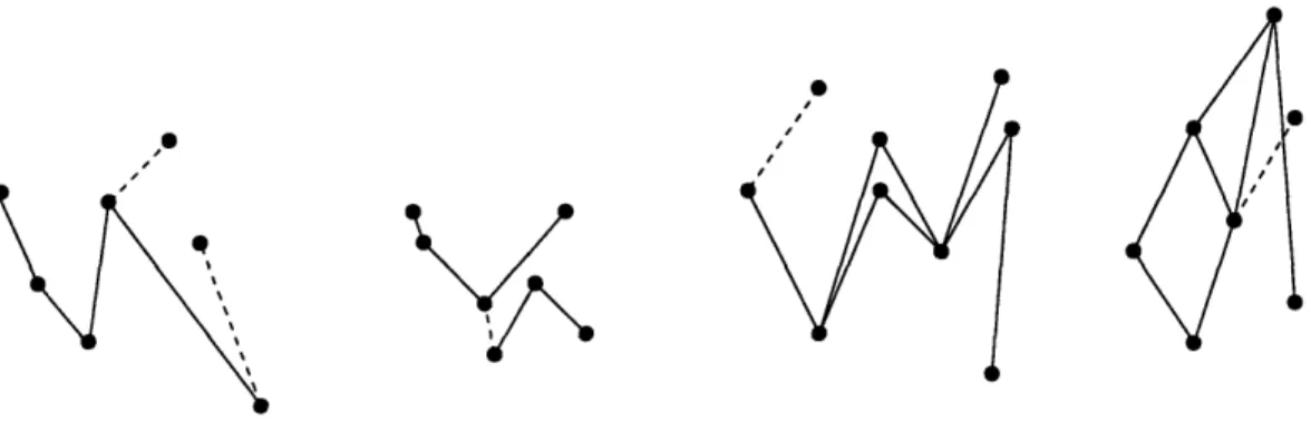
'S

Figure 2-1: The structure of G': G' has 4 connected components. Strong edges are shown with solid lines, and weak edges with dotted lines. There are no strong edges between the connected components. Components do not "overlap." Each weak edge is adjacent to at least one strong edge.

For an edge (v, w) E E' which is oriented up, such that vl < wl, we have

w

2

-

2

+

E

D[v, w]

>

w

2

-

2

-

(2.2)

Claim 2.1.5 By fixing the orientation of an edge of G' we also fix the orientation of

all the other edges in the same connected component of G'.

Proof: We first show that if we know the orientation of an edge e, then we can

also determine the orientation of any adjacent edge if both e and the adjacent edge are not weak edges. By setting the orientation of an edge and repeating this process we can determine the orientation of all the edges in the connected component.

Without loss of generality, we assume that the edge (v, w) E E' (wl _ vi) is

oriented up: w2 - v2 > w1 -

v

1. Also let (w, t) E E'.

If (w, t) is a strong edge and (w, t) is oriented up, by using (2.2) multiple times we get

Since (w, t) is a strong edge, D[w, t] > 3e, therefore

D[v, t] > D[v, w] (2.3)

Using the fact that (v, w) is an edge and (w, t) is a strong edge (i.e., D[v, w] >

wl - vI + and D[w, t] > It1 - wjl + 3c), we get

D[v,t] > (w, - vl) + It, - wl + E > Itl - v11 + E (2.4)

If (w, t) is a strong edge and (w, t) is oriented down, we have

D[v, t] 5 IIt-vI(,+E < max{Itl-vli+e, D[v, w]+E-D[w, t]+cE < max{Itl-vlI+E, D[v,

w]}

(2.5) Since equations (2.3) and (2.4) contradict equation (2.5), we can determine whether

(w, t) is oriented up or down.

If (w, t) is a weak edge and (v, w) is a strong edge, then by a similar argument we can determine the orientation of (w, t). If a connected component of G' contains only one connected component of G, we can determine the orientation of all the strong edges first and then the orientation of the weak edges. If a connected component of G' contains two connected components of G, then these two components must overlap (by the way we add weak edges), which means that there is a weak edge connecting them. This means that we can determine the orientation of the strong edges in the first component, then the orientation of a weak edge between the two components, then the orientation of the strong edges of the second component, and finally the orientation of all the remaining weak edges. The same argument applies to the case when the connected component of G' is composed of several connected components

of G. 0

Claim 2.1.6 Given the orientation of all the strong edges, we can compute a

Proof: We construct the following linear program:

Min 6

subject to

Dip, q] - 6 > q2 - P2 > D[p, q] + ±, if (p, q) E E is oriented up and q, > pi D[p, q] - 6 > P2 - q2 • D(p, q] + 6, if (p, q) E E is oriented down and ql Ž pi

-D[, q] - 6 < q2 -p2 < D[p, q] + 6, if (p, q) • E

First note that, if we were to have all the edges (including the weak ones) in

E, we would get an optimal solution. However, we know the orientation of only

the strong edges, and this gives a approximation solution: It is clear that a 3-approximation solution that satisfies the orientation given is a feasible solution for this linear program. It is also clear that any solution of this program is an embedding

with error of at most max(j*, 3e) and 6* < 3e. 0

By using Claims 2.1.5 and 2.1.6 we can get an approximate solution to the problem. But what if we have several connected components in G'? We will prove that no matter what relative orientation we take between the edges of the components, we will still get a constant approximation solution. So, the algorithm is as follows: we choose an arbitrary orientation to one edge from each connected component, and by using Claims 2.1.5 and 2.1.6 we get an approximate solution.

Claim 2.1.7 There is a 5-approximation solution for every relative orientation

be-tween the edges of the components.

Proof: Let

f

be an optimal embedding. Let C1, C2, C3, -.. , Ck be the connected

components of G', from the ones with the smallest x coordinate to the ones with higher x coordinate: Vi, if v E Ci and w E Ci+l, then vl 5 wl.

Choose any relative orientation of the components. Let the function s : {1, 2, ... , k} -k {0, 1} denote the relative orientation of our arbitrary choice to the optimal embed-ding f: s(i) = 1 if the orientation of the component Ci is different in f than in our

arbitrary selection; s(i) = 0 otherwise.

We are going to start with an optimal solution and modify it to get a feasible solution that has the given relative orientation, with error of at most 5e:

We are going to modify f incrementally from the first component to the last. Without loss of generality we can assume s(1) = 0. (If s(1) = 1 we can flip (or reflect) f by the x axis, flipping each s(i) and still having an optimal embedding.)

We repeat the following steps for i from 2 to k: If s(i) = 0, then we go to the next component Ci+I.

If s(i) = 1, then we will flip all the points in k=i Cj by a certain line parallel to

the x axis. This flip will change the values of s(j) for all j > i. The line by which we are going to flip the points is computed as follows:

* Let p be a point in

U~fl C

3 that maximizes pi

+

p2: Vv E

U=l

C, p

1

+P2

V1 + V2

-* Let q be a point in j=l Cj that maximizes qi -q

2

: Vv E Ui-I Cj, qi -q

2

>

V1--v 2

.

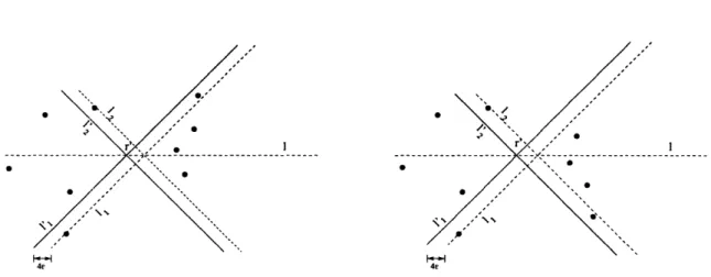
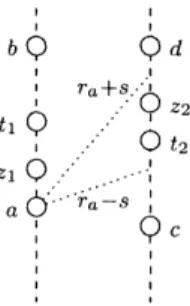
* Let 11 be the line of slope -7r/4 that passes through p, and let 12 be the line of slope -r/4 that passes through q. Let the point r denote the intersection of li with 12. Let I be the line through r that is parallel to the x axis.

* Flip the points in j=i Cj by

1:

for all v E

Uj=

C,

v' = 2r2 - 2

It is easy to see that by performing this flip operation on f we change only the distances between v and w for v

E

U=l

1 Cj and w E

U~=i

Cj.

The question

is:

by

how much? Since there are no strong edges between the components, for such v and

w, we have:

D[v, w] • Iv, - w1I + 3e (2.6)

If v E Ci-1, then by the flips up to this step, the distance between v and w has remained the same as in the original embedding:

Combining equations (2.6) and (2.7) we get

(w2 -

v

2

1

<

D[v, w]

+

e

< IW, - vi•

+

4E

(2.8)

Let v' be the point 4E to the left of v: v' = vl - 4E and v = v2. Let d' be the line

of slope 7r/4 that goes through v' and d" be the line of slope -7r/4 that goes through V'.

It is easy to see that equation (2.8) implies w is located beneath d' and above d". (See Figure 2-2)

Figure 2-2: The points w E Uj=i Cj are located beneath d' and above d".

This holds for each v E Ci-1. Therefore each w E Uk Cj is located between these wedges. Now, our line I is chosen such that after we flip the points w E

U=i

Cj,

they will remain between these wedges, such that equation (2.8) remains true after the flip. 4 Since we do not change the x coordinates and the original f is a solution 4_{The intersection of the space between pairs of wedges has the same shape as the space between}

2 wedges and I divides this intersection into 2 symmetrically equal pieces. 4E

with error e we know that

D[v, w] + E > •wl - viJ (2.9)

Combining equations (2.8) and (2.9), we get

Iw2

-

V21

<

[1 -

vl

+ 4e

<

D[v, wI + 5E

IS

---

---

₀

--S

4e 4e

Figure 2-3: The points in U= Cj will remain between the two lines (wedges) l1 and

l2 after the flip.

In addition, since for the next flips, the points that are being flipped are inside an even more restrictive space between two wedges, they will not leave the space between the two wedges and equation (2.8) will remain true after we have completed all the flips. Again, since equation (2.9) is also true, we can combine them and get that Iw2 - v21 5 D[v, w] + 5E after all the flips are completed. By applying this

argument to v E C1, v E C2,..., we conclude that for all points v, w, wl _ vl, we have w2 - V21 : • D[v, w] + 5E. Since we have no strong edges between the components,

for v E Ci, w E Cj, i = j, Jvi - wlI > D[v, w] - 3c. This implies that for two points

from different components, the distortion in our construction is at most 5e. Since we preserve the distances between points from the same component, we have constructed an embedding with distortion of at most 5E for an arbitrary relative orientation of the edges between the connected components.

U

P

Finally, we apply Claim 2.1.6 to produce a 5-approximation solution. We know that for our orientation there is an embedding with error 5E and this is a feasible solution for our linear program.

2.1.4

The Final Algorithm

So far, we assumed we know certain points (the pair of points that give the diameter, etc). To satisfy this assumption, we will iterate over all possible choices (a polynomial number of such choices). The total running time of the algorithm is O(log diamn6LP) -7-where diam is the value of the diameter of P and LP is the time to solve a linear program with n variables and O(n) constraints. Thus, the running time is polynomial in n.

2.1.5

The general case

The main idea is to fix the x coordinates of the points and then to use the algorithm from the previous section. We do not need to guess the x coordinates exactly. If we guess them within cE for a constant c, it will be enough to get a constant approxima-tion algorithm for the general case.

Let p and q denote the diameter. Let f be an optimal embedding with error E.

Without loss of generality we have p = (0, 0) and we assume that the diameter is given by ql - pi.

Let A be the set of points v E P - {p, q} for which the following equation is true:

D[p, q] + ke > D[p, v] + D[v, q]

A = {v E P - {p, q} : D[p, q] + ke 2 D[p, v] + D[v, qJ}

for a fixed constant k which we will chose later.5

5

Note that for v E A, we have the following two inequalities:

v

i

< D[p, v] + E

vi > D[p, q]

-

D[v, q]

-

2E > D[p, v]

-

(k +

2)e

It follows that by fixing vi = 2D- ,v]-(k+l)e = Dj, v] - (k+), we are within an additive factor of (k3) from the value of vl in the optimal embedding

f.

It is clear that if A = P - {p, q} then we can guess the x coordinate of all the

points in A and then by reducing the problem to the special case with e' =- (k+3) we get a (k+3) --approximation algorithm.

But what happens if P - A

#

0? We break our analysis into two cases:

Case 1

For this case we assume that for all points v E P-A-{p, q} we have either Ilp-v 1, =

Ilp

- vl or lIq - vilI =

q11

- v1J.

Partition the points of P - A

B

=

{v

- {p, q} into three sets:

E

P -

A -

{p,q}

:

p

- vll

op

=

l -

,vi

)

C = {vE P

-

A - {p,q} :

Iq

- voo = 1q1 - v1q and

v2 - 2

Ž!

0}

D

=

{v E

P-

A - {p,q} :

Iq

- vJ

= ql- vl

and v

2 -p 2 <

0}

Note that this is a partition: If BnC 4

0

then there exists v E BnC, and we have

D[p, q] > ql--pl-c

=

ql-vl+vl-pl

-=

I q-vloo+ljv-ploo-E

>

D[q, v]+D[p, v]-3E

which implies v E A, which is a contradiction.

The idea is to choose certain points to decide for each point v E P - A - {p, q}

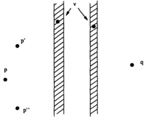
within an additive error of ce for some constant c. p" p p,, V 4/ 4 4/ 4 4/ 4/

Figure 2-4: If v E B then v is restricted to the right stripe of width 26. If v E C U D then v is restricted to the left stripe of width 46. Since v is not in A, we know that the distance between the stripes is at least (k - 2)E

Let the point p' E C be such that p' = minVEc vl + v2 and the point p" E D such

that p" = minvED vl - v2. Of course, p' or p" may not even exist, but those cases are

easier to handle and the proof is basically the same for them as well. Since p' ý A, we have

Dip', q] > D[p, q] + kE - D[p, p']

(2.10)

Since p' E C, we have the following inequalities

P2 -

E <

Dip',

p]

p2 +

(2.11)

Di[p,

q] - D[p', q] - 2E

<

p' < D[p, q] - D[p', q] + 2E (2.12) By combining (2.10) with (2.12) we get that p' < D[p,p'] - (k - 2)e. Using (2.11) we get that

p < p2 - (k - 3)E (2.13)

I

For a point v E B, we have Dp', v] > v, - p' I - e

>

Dip,

v]

- 2e - p',

> D[p, v] - P + (k - 5)E > D[p, v] - D[p,p'] + (k - 6)6 Also, by (2.13) by (2.11) (2.14)

Dip', • > Ii - P'l - 6

> D[p, v] - 2

-p'

> Dip, v] - Dip, q] + Dip', q] - 46 by (2.12)

(2.15)

For a point v

E C,

we have D[p', v]

<

ip',

vloo + F Inax(vi - p', v2- p2)

+

by

the way p' was chosen.

If I p', vli,- =

v

2

-

p2,

we have

D[_p', v] V2 - 2 +- 2

<

Dp,v]

-

p +

2c

< Dip, v]

-

Dip,p'] + 3c

by (2.11) (2.16)

If D[p', v] = vl - p' + e, we have

D[p,

v]

=

v

1

-

P

+

< D[p, q]- D[q, v] - p +3 < D[p, v] - (k - 3)E - p' by (2.10)

<

Dp, v

-

(k -3)

- (D[p, q] - D[p', q] - 2E) by (2.12) = D[p, v] - D[p, q] (2.17) + D[p', q] - (k - 5)E

Note that if k > 9, equations (2.17) and (2.15) are contradictory.

We can also obtain similar equations for v E D by replacing p' with p" in the above argument. We use these observations to prove the following claim:

Claim 2.1.8 We can determine which points are in B and which ones are in C U D

if k > 9.

Proof: If v E B, by (2.14) and (2.15), the following equations are true:

D[p', v] D[p, v] - D[p, p'] + (k - 6)E

Dip', v] D[p, v] - D[p, q] + D[p', q] - 4e D[p", v]

Ž

D[p, v] - D[p, p"] + (k - 6)c

Dfp", v] > D[p, v] - D[p, q] + Dfp", q] - 4e

If v E CUD then either (2.16) or (2.17) is true (for p' if v E C or for p" if v E D) which implies that at least one of the above 4 equations is false. Therefore we say that v E B if all the about 4 equations are true, and v E C U D otherwise. 0

Case 2

For this case we assume that there exists a point r E P- {p, q} for which the following

is true:

jjp-.rjlo

>

Ipi-rl

and |jq-rlJoo > Iql-r

1

j. It follows that lip-rloo

= IP2-r 2J

and

liq

- rl

o

=

Iq2

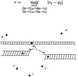
- r2j.

Let r be such a point that maximizes

1r

2- P21:

r = max vEP llp-rlloo=p2-r21 llq-rllo=1q2-r21

Ir

2

- P2

P I I I I I I IIIII //

~

/ II

IL÷17111T11T

Figure 2-5: If v E B then v is restricted to the upper stripe of width 2E. If v E C then v is restricted to the lower right stripe of width 4e. If v E D then v is restricted to the lower left stripe of width 4E

For this case, we will fix the y coordinate instead. The method we will use is going to be very similar to the method used for case 1. We partition the points of

P - {p, q, r} into four sets as follows:

A = {v E P-{r, p, q} : D[r, p]+kc > D[r, v]+D[v, p] or D[r, q]+kE > D[r, v]+D[v, q]}

B

=

{v

E

P

-

A

-

{r,p,q}

:

1r

-

vll0

=

-

r

2

-

v

2

I}

L

C = {v E P - A - {r,p,q} :

I1r

- vl00 =

Irl

- vI and vi - rl 01

D = {v E P - A - {r,p,q} :

JIr

- vllo =

Jr

1 -

v

1 and vi - ri < 0}

Claim 2.1.9 If v E C we can determine its y coordinate within an additive factor of 2E

Proof: By the way of contradiction, we suppose that

I

q - vll = - v-1 1. Then

D[v, q] Ž q1 - vy - E. It follows that D[r, q] Ž q1 - ri - E > ql - vi + v1 - q1 - e >

D[r, v] + D[v, q] - 3e. But for k > 3, this implies v E A, which contradicts the fact that v E C.

Therefore, we know that |Iq - vl 0 = jq₂ - v21. If v₂ > q2 we have that v, > v₂ >

q2 > q1 which means that the diameter is given by the pi - vi , again impossible. Therefore,

jjq - vjj00 = q - V2

Using this observation, we have the following two bounds on v2: D[r, q] -D[r, v] -2e < v2 _ D[r, q] - D[r, v] + 2E and we can guess v2's real value within an additive distance

of 2E by setting v2 = D[r, q] - D[r, v]. 0

Similarly by replacing q with p in the above proof, if v E D we can also determine its y coordinate within an additive factor of 2c.

We shift everything and flip it by the y axis if necessary such that, r = (0, 0) and P2 > 0. Note that this implies that q2 > 0 (if q2 < 0 then we would have

1P2

- q21 = IP2 - r2l + Ir2 - q21 >

Ilp

- r1I +

jr,

- qj =

Ilp

- qll = diam(P), which

is a contradiction) and that every v E B has v2 > 0 (because we chose r such that it

maximizes r2 - P2). We proceed as before: we pick certain points to help us decide

for each point in which set it belongs to. If we can decide that, we can approximate for each point its y coordinate within a constant times E.

Let the point r' E C be such that r' = minVEC vI + v2 and the point r" E D such

cases are easier to handle and the proof is basically the same for them as well. Since r' 0 A, we have

D[r', q] > D[r, q] + kE - D[r, r'] (2.18)

Since r' E C, we have the following inequalities

r -E < D[r',r] r' +E (2.19)

(2.20)

D[r, q] - D[r', q] - 2e < r'2 D[r, q] - D[r', q] + 2E

By combining (2.18) with (2.20) we get that r' < D[r, r'] - (k - 2)e. Using (2.19) we get that

(2.21)

r/ < r' - (k - 3)

For a point v E B, we have

D[r', v] _ Jv2 - r'2 - E " D[r, v] - 2E - r'2 > D[r, v] - r' + (k - 5)E > D[r, v] - D[r, r'] + (k - 6)E Also, by (2.21) by (2.19) (2.22)

D[r',

v]

2

-

r'I - E

> D[r, v] - 2E - r'2 > D[r, v] - D[r, q] + D[r', q] - 4E by (2.20) (2.23)

For a point v E C, we have D[r', v] • max(v2 - r', vl - r') + e by the way r' was

If IIr', vlloo = V1 - r', we have

D[r', v] < vl - r' + e SD[r, v] - r + 2e

< D[r, v] - D[r, r'] + 3e by (2.19) (2.24)

Note that if k > 9, equations (2.22) and (2.24) are contradictory. If

IIr',

vlloo = v2 - Tr, we have

D[r', v]

•

v2 - r2 + 6 < D[r, q] - D[q, v] - r' + 3e < D[r, v] - (k - 3) - r by (2.18)

<

Dir, v] - (k - 3)c - (D[r, q] - D[r', q] - 2E) by (2.20) = D[r, v] - D[r, q] + D[r', q] (2.25) - (k - 5)e

Note that if k > 9, equations (2.25) and (2.23) are contradictory.

We also have very similar equations for v E D by using r". We use these observa-tions to prove the following claim.

As before, we can use these equations to determine which points are in B and which ones are in C U D. However, in this case, we should also distinguish between

C and D. We make the following observation:

Claim 2.1.10 If D[q, v]+D[v, r']

<

D[r', q]+3E or

D[,

v]+D[v, r"]

<

D[r",p]+3E we

can approximate v2 within a factor of 3e. Otherwise, if v E C, then D[r', v] < D[r", v]

Proof: First note that D[r', r"] has to be pretty large:

D[r', r"] >

r'

- r,

+

ri r"

-2

D[r', r] + D[r", r] - 3E > D[r, q] - D[r', q] + D[r, p] - D[r",p] + (2k - 3)E > q2 -2 - E -

(q

2 - r2 + E) +P2- - 2 - - (q2 - r2

+

E)

+

(2k - 3)c r2- r2 +r2 - r2 + (2k - 7)c > (2k - 7) (2.26)

We break our proof into three cases:

* Case 1: D[q, v] + D[v, r'] _ D[r', q] + 3E

First note that we know that

v2 _ q2 - D[q, v] -

c

> D[r, q] - D[q, v] - 2E (2.27)

We also have that

v2 r' + D[v, r'] + E (2.28)

_ D[r, qJ - D[q, r'] + D[v, r'] + 3e (2.29)

• D[r, q] - D[q, v] + 6e (2.30)

2 Therefore, as before, we can approximate v2 within an additive error of 4e by

setting

v2

=

D[r, q] - D[q, v] + 2E.

* Case 2: D[p, v] + D[v, r"] 5 D[r", p] + 3c

The analysis of this case is analogous to the one above. (replace r' by r" and q by p).

*

Case 3: If Ijr' - vlIoo = v2 - r' we have that D[q, v]

+

D[v, r'] < D[r', q]

+

3e,

which falls into case 1. Therefore, we know that I Ir ' - v11o = vl - r'. In that case,

D[r", v] vI - r' + r' - r - E

D[v, r'] + r'

-

r" - 2E

Ž D[v, r'] + D[r', r"] - 3E

> D[v, r'] + (2k - 10)e by (2.26) (2.31)

Therefore, for v E C we have D[r", v] > D[v, r'] if k > 5. Symmetrically, for v E D

we have D[r", v] < D[v, r'] for k > 5.

We conclude that it is either the case that we can approximate v2 within 4e (case

1 or 2) or we can compare D[v, r"] with D[v, r'] to determine if v E C or v E D which implies we can approximate v2 within additive error 2E.

Using this observation we can easily distinguish between points in C and points in D. For the points in v E C we fix the y coordinate as v2 = D[r, q] - D[q, v] and

for the points v E D, v2 = D[r, p] - D[p, v].

2.1.6

Conclusions

In this section, we showed how to approximate within a constant factor an embedding of an arbitrary metric into a two-dimensional space where distances are computed using the 11 norm with the notion of an additive error e. Our constant is 30, but by combining the general case with the special case more carefully, we believe can get the constant down to 19, by just a tighter analysis in the constants.

Future Work. We believe the distortion and the running time can be improved further. We also believe that the same technique might be extended to get the same result for other norms (e.g., 12) or multiplicative error. It would also be of interest to

extend this result for higher dimensions - let's say three-dimensional space. It should also 1w, noticed that in the case of the 12 norm, while we don't know how to prove claim (2.1.7) with additive error, it is easy to prove it with multiplicative error and we can

obtain an embedding f : P

-+

R2

, for which D[p, q]

•

IIf(p)

- f(q)(1

2

_ aD[p, q] +bE*,

where a and b are absolute constants.

Acknowledgements. The author would like to thank Piotr Indyk and Sariel Har-Peled for numerous comments on early drafts of the results and in particular to Piotr Indyk for useful discussions.

2.2

Constant-factor approximation of the average

distortion of embedding a metric into the line.

Credits: The results in this section is work done with Piotr Indyk and Yuri Rabi-novich in the autumn of 2002. The results haven't been published yet.

The average distance of D, av(D) = 1/n2 -x,EP D(x,y), is the average of

distances of n2 ordered pairs of points. In this section we consider non-contracting

(or expanding) embeddings f of metric D into a host space Y, i.e., such that the induced submetric D' of Y dominates D (no distance decreases).

Let avy(D) be the minimum of av(D') over all such D'. We will show that, given

D, one can 0(1)-approximate avline(D), where the host space is R.

The average distortion of f is defined as av(D')/av(D) > 1. The median of the metric D on P be the point p E P minimizing the expression 1/n ZXEP D(p, x); it will be denoted by med. Observe that for a set of points on a line, the standard order-median coincides with the metric-median.

We start with the following simple fact:

av(D)> Ž I D(med, x) 1/2 --av(D) . (2.32)

xEP