Publisher’s version / Version de l'éditeur:
Proceedings of the 23rd Canadian Conference on Artificial Intelligence (AI 2010),
pp. 184-195, 2010
READ THESE TERMS AND CONDITIONS CAREFULLY BEFORE USING THIS WEBSITE. https://nrc-publications.canada.ca/eng/copyright
Vous avez des questions? Nous pouvons vous aider. Pour communiquer directement avec un auteur, consultez la première page de la revue dans laquelle son article a été publié afin de trouver ses coordonnées. Si vous n’arrivez pas à les repérer, communiquez avec nous à [email protected].
Questions? Contact the NRC Publications Archive team at
[email protected]. If you wish to email the authors directly, please see the first page of the publication for their contact information.
NRC Publications Archive
Archives des publications du CNRC
This publication could be one of several versions: author’s original, accepted manuscript or the publisher’s version. / La version de cette publication peut être l’une des suivantes : la version prépublication de l’auteur, la version acceptée du manuscrit ou la version de l’éditeur.
For the publisher’s version, please access the DOI link below./ Pour consulter la version de l’éditeur, utilisez le lien DOI ci-dessous.
https://doi.org/10.1007/978-3-642-13059-5_19
Access and use of this website and the material on it are subject to the Terms and Conditions set forth at
Automatic parameter settings for the PROAFTN classifier using Hybrid
Particle Swarm Optimization
Al-Obeidat, Feras; Belacel, Nabil; Carretero, Juan A.; Mahanti, Prabhat
https://publications-cnrc.canada.ca/fra/droits
L’accès à ce site Web et l’utilisation de son contenu sont assujettis aux conditions présentées dans le site LISEZ CES CONDITIONS ATTENTIVEMENT AVANT D’UTILISER CE SITE WEB.
NRC Publications Record / Notice d'Archives des publications de CNRC:
https://nrc-publications.canada.ca/eng/view/object/?id=bdf5b4f8-cc28-448e-90b8-af444df5189f https://publications-cnrc.canada.ca/fra/voir/objet/?id=bdf5b4f8-cc28-448e-90b8-af444df5189fClassifier using Hybrid Particle Swarm Optimization
Feras Al-Obeidat, Nabil Belacel, Juan A. Carretero, and Prabhat MahantiUniversity of New Brunswick, Canada
Abstract. In this paper, a new hybrid metaheuristic learning algorithm is intro-duced to choose the best parameters for the multi-criteria decision making algo-rithm (MCDA) called PROAFTN. PROAFTN requires values of several parame-ters to be determined prior to classification. These parameparame-ters include boundaries of intervals and relative weights for each attribute. The proposed learning algo-rithm, identified as PSOPRO-RVNS as it integrates particle swarm optimization (PSO) and Reduced Variable Neighborhood Search (RVNS), is used to automati-cally determine all PROAFTN parameters. The combination of PSO with RVNS allows to improve the exploration and exploitation capabilities of PSO by setting some search points to be iteratively re-exploited using RVNS. Based on the gen-erated results, experimental evaluations show that PSOPRO-RVNS outperforms six well-known machine learning classifiers in a variety of problems.
Key words: Knowledge Discovery, Particle swarm optimization, Reduced Vari-able Neighborhood Search, Multiple criteria classification, PROAFTN, Super-vised Learning.
1
Introduction
Data classification in machine learning algorithms is a widely used supervised learning approach. It requires the development of a classification model that identifies behaviors and characteristics of the available objects to recommend the assignment of unknown objects to predefined classes [3]. The goal of the classification is to accurately assign the target class for each instance in the dataset. For instance, in medical diagnosis, patients are assigned to disease classes (positive or negative) according to a set of symptoms. In this context, the classification model is built on historical data and then the generated model is used to classify unseen instances.
Multi-criteria decision analysis (MCDA) [22] is another field that addresses the study of decision making [14] and classification problems. In recent years, the field of MCDA has been attracting researchers and decision-makers from many areas, including health, data mining and business [26]. The classification problem in MCDA consists of the formulation of the decision problem in the form of class prototypes that are used for assigning objects to classes. Each prototype is described by a set of attributes and is considered to be a good representative of its class [17].
PROAFTN is a relatively new MCDA classification method introduced in [6] and belongs to the class of supervised learning algorithms. PROAFTN has successfully been
applied to many real-world practical problems such as medical diagnosis, asthma treat-ment, and e-Health [7, 9, 10]. However, to apply the PROAFTN classifier, the values of several parameters need to be determined prior to classification. These parameters in-clude the boundaries of intervals and the relative weight for each attribute. This consists of the formulation of the decision problem in the form of prototypes – representing each class – to be used for assigning each object to the target class.
Recently, some related work introduced in [2] was done to improve PROAFTN’s performance. There, the unsupervised discretization algorithm k-means and a Genetic Algorithm (GA) were used to obtain the best number of clusters and optimal proto-types obtained after completion of a clustering process. Here, a new method is pro-posed based on particle swarm optimization (PSO) and Reduced Variable Neighbor-hood Search (RVNS) to obtain all PROAFTN training parameters. This study proposes a different approach than the one proposed in [2] in that the formulation of the optimiza-tion problem is entirely different. The integrating or hybridizaoptimiza-tion of PSO and RVNS significantly improves the exploration and exploitation strategies.
The rest of the paper is organized as follows: in Section 2, the PROAFTN method as well as the PSO and RVNS algorithms are briefly presented. In Section 3, the pro-posed approach PSOPRO-RVNS to learn PROAFTN is introduced. The description of the datasets, experimental results, and comparative numerical studies are presented in Section 4. Finally, conclusions are summarized in Section 5.
2
Overview of PROAFTN, PSO and RVNS
2.1 PROAFTN Method
PROAFTN belongs to the class of supervised learning algorithms [6]. Its procedure can be described as follows. From a set of n objects known as a training set, consider a is an object which requires classification; assume this object a is described by a set of m attributes{g1, g2, . . . , gm} and let {C1,C2, . . . ,Ck} be the set of k classes. The different
steps of the classification procedure follow.
Initialization For each class Ch, h= 1, 2, . . . , k, a set of Lhprototypes Bh= {b1h, bh2, . . . , bhLh} are determined. For each prototype bh
i and each attribute gj, an interval[S1j(bhi), S2j(bhi)]
and the preference thresholds d1
j(bhi) ≥ 0 and d2j(bhi) ≥ 0 are defined where S2j(bhi) ≥
S1
j(bhi), with j = 1, 2, . . . , m and i = 1, 2, . . . , Lh.
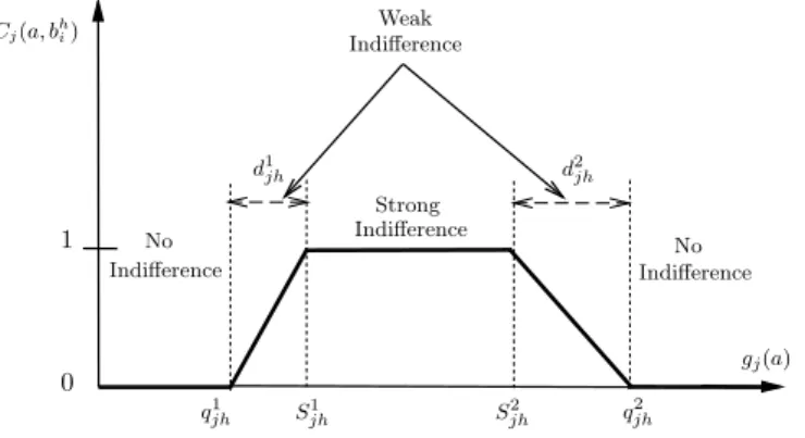
Figure 1 depicts the representation of PROAFTN’s intervals. To apply PROAFTN, the pessimistic interval[S1
jh, S
2
jh] and the optimistic interval [q
1
jh, q
2
jh] for each attribute
in each class need to be determined [8], where:
q1jh= S1jh− d1jh q2jh= S2jh+ d2jh (1) applied to: q1jh≤ S1jh q2jh≥ S2jh (2) Hence, S1 jh= S1j(bhi), S2jh= S2j(bhi), q1jh= q1j(bhi), q2jh= q2j(bhi), d1jh= d1j(bhi), and d2jh= d2j(bh
i). The following subsections explain the different stages required to classify object
Cj(a, bhi) Indifference Indifference 1 0 S2 jh q2jh q1jh gj(a) d1jh d2jh Strong Weak Indifference No Indifference No S1 jh
Fig. 1. Graphical representation of the partial indifference concordance index between the object
aand the prototype bhi represented by intervals.
Computing the fuzzy indifference relation I(a, bh
i) The initial stage of the
classifica-tion procedure is performed by calculating the fuzzy indifference relaclassifica-tion I(a, bh i). The
fuzzy indifference relation is based on the concordance and non-discordance principle which represents the relationship (i.e., the membership degree) between the object to be assigned and the prototype [5, 8]. It is formulated as:
I(a, bhi) = Ã m
∑
j=1 wjhCj(a, bhi) ! m∏
j=1 ³ 1− Dj(a, bhi)wjh ´ (3) where wjh is a weighting factor that measures the relative importance of a relevantattribute gj of a specific class Ch: wjh∈ [0, 1] and ∑mj=1wjh= 1 Also, Cj(a, bhi), j =
1, 2, . . . , m, is the degree that measures the closeness of the object a to the prototype bh i
according to the attribute gj. The calculation of Cj(a, bhi) is given by:
Cj(a, bhi) = min{C1j(a, bhi),C2j(a, bhi)}, (4)
where C1j(a, bh i) = d1j(bh i) − min{S1j(bhi) − gj(a), d1j(bhi)} d1 j(bhi) − min{S1j(bhi) − gj(a), 0} and C2j(a, bh i) = d2j(bh i) − min{gj(a) − S2j(bhi), d2j(bhi)} d2j(bh i) − min{gj(a) − S2j(bhi), 0}
Finally, Dj(a, bhi) is the discordance index that measures how far object a is from
pro-totype bhi according to attribute gj. Two veto thresholdsε1j(bhi) andε2j(bhi) [6], are used
to define this value, where the object a is considered perfectly different from the proto-type bhi based on the value of attribute gj. Generally, the determination of veto
thresh-olds through inductive learning is risky. These values need to be obtained by an expert familiar with the problem. However, this study is focused on an automatic approach.
Therefore, the effect of the veto thresholds is eliminated by setting them to infinity. As a result, only the concordance principle is used. Thus, Eq (3) is summarized as:
I(a, bhi) = m
∑
j=1
wjhCj(a, bhi) (5)
To sum up, three comparative procedures between object a and prototype bhi accord-ing to attribute value gjare performed (Fig. 1):
– case 1 (strong indifference): Cj(a, bhi) = 1 ⇔ S1jh≤ gj(a) ≤ S2jh
– case 2 (no indifference): Cj(a, bhi) = 0 ⇔ gj(a) ≤ q1jh, or gj(a) ≥ q2jh
– case 3 (weak indifference): The value of Cj(a, bhi) ∈ (0, 1) is calculated based on
Eq. (4). (i.e., gj(a) ∈ [q1jh, S1jh] or gj(a) ∈ [S2jh, q2jh])
Evaluation of the membership degree δ(a,Ch) The membership degree between
object a and class Ch is calculated based on the indifference degree between a and its nearest neighbor in Bh. The following formula identifies the nearest neighbor:
δ(a,Ch) = max{I(a, bh
1), I(a, bh2), . . . , I(a, bhLh)} (6) Assignment of an object to the class The last step is to assign object a to the right class Ch. To find the right class the following decision rule is used:
a∈ Ch⇔δ(a,Ch) = max{δ(a,Ci)/i ∈ {1, . . . , k}} (7) 2.2 Particle Swarm Optimization Algorithm
Particle Swarm Optimization (PSO) is a population-based and adaptive optimization method introduced by Eberhart and Kennedy in (1995) [13]. The fundamental concepts of PSO are intuitively inspired by social swarming behavior of birds flocking or fish schooling. Thus, compared with Genetic Algorithms (GAs), the evolution strategy in PSO is inspired from social behavior of living organisms, whereas the evolutionary strategy of GAs is inspired from biological mechanisms (i.e., mating and mutation). More specifically, in the PSO evolutionary process, potential solutions, called particles, move about the multi-dimensional search space by following and tracking the current best particles in the population.
¿From an implementation perspective, PSO is easy to implement and computation-ally efficient compared to other EAs algorithms [18, 20]. The general procedure of PSO is outlined in Algorithm 1.
Functionality of PSO Each particle in the swarm has mainly two variables associated with it. These variables are: the position vector xi(t) and the velocity vector vi(t). Thus,
each particle xi(t) is represented by a vector [xi1(t), xi2(t), . . . , xiD(t)] where i is the
index number of each particle in the swarm, D represents the dimension of the search space and t is the iteration number.
Algorithm 1 PSO Evolution Steps
Step 1: Initialization phase, Initialize the swarm Evolution phase
repeat
Step 2: Evaluate fitness of each particle
Step 3: Update personal best position for each particle Step 4: Update global best position for entire population Step 5: Update each particle’s velocity
Step 6: Update each particle’s position
until (termination criteria are met or stopping condition is satisfied)
During the evolutionary phase, each of the Npop particles in the swarm is drawn
toward an optimal solution based on the updated value of vi and the particle’s current
position xi. Thus, each particle’s new position xi(t + 1) is updated using:
xi(t + 1) = xi(t) + vi(t + 1) (8)
The new position of the particle is influenced by its current position and velocity, the best position it has visited (i.e., its own experience), called personal best and denoted here as PBest
i (t), and the position of the best particle in its neighborhood, called the
global best and represented by GBest(t). At each iteration t, the velocity v
i(t) is updated
based on the two best values PBest
i (t) and GBest(t) using the formula,
vi(t + 1) = ϖ(t)vi(t)
| {z }
inertial parameters
+ τ1ρ1(PBesti (t) − xi(t))
| {z }
personal best velocity components
+ τ2ρ2(GBest(t) − xi(t))
| {z }
global best velocity components
(9)
whereϖ(t) is the inertia weight factor that controls the exploration of the search space. Factorsτ1andτ2are the individual and social components/weights, respectively, also
called the acceleration constants, which change the velocity of a particle towards the PBesti (t) and GBest(t), respectively. Finally, ρ
1 andρ2 are random numbers between
0 and 1. During the optimization process, particle velocities in each dimension d are evolved to a maximum velocity vdmax(where d= 1, 2 . . . , D).
2.3 Reduced Variable Neighborhood Search (RVNS)
RVNS is a variation of the metaheuristic Variable Neighborhood Search (VNS) [15, 16]. The basic idea of the VNS algorithm is to find a solution in the search space with a sys-tematic change of neighborhood. In RVNS, two procedures are used: shake and move. Starting from the initial solution (the position of prematurely converged individuals) x, the algorithm selects a random solution x′from first neighborhood. If the generated x′ is better than x, it replaces x and the algorithm starts all over again with the same neigh-borhood. Otherwise, the algorithm continues with the next neighborhood structure. The pseudo-code of RVNS is presented in Algorithm 2.
Algorithm 2 RVNS Procedure
Require:
Define neighborhood structures Nkfor k= 1, 2, . . . , kmax, that will be used in the search
Get the initial solution x and choose stopping condition repeat
k← 1
while k< kkmaxdo
Shaking:
Generate a point x′at random from the kth neighborhood of x(x′∈ Nk(x))
Move or not:
if x′is better than the incumbent x then x← x′ k← 1 else set k← k + 1 end if end while
until stopping condition is met
3
Problem Formulation
In most cases, and depending on the population size, PSO may not be able to explore and exploit the entire search space thoroughly. To improve the exploitation process, RVNS forces individuals to ‘jump’ to another location in the solution space while PSO allows these points to continue the search using past experience. As discussed earlier, to apply PROAFTN, the intervals[S1
jh, S2jh] and [q1jh, q2jh] that satisfy the constraints in
Eq. (2) and the weights wjhin Eq. (5) are to be obtained for each attribute gjbelonging
to each class Ch. In this study, the induction of weights is based on the calculation of
entropy and information gain [25]. An entropy measure of a set of objects is calculated as Entropy= − ∑C
i=1(pi) log2(pi), where piis the proportion of instances in the dataset
that take the ithvalue of the target attribute and C represents the number of classes.
To simplify the constraints in Eq. (2), a variable substitution based on Eq. (1) is used. As a result, parameters d1jhand d2jhare used instead of q1jhand q2jh, respectively. Therefore, the optimization problem, which is based on maximizing classification ac-curacy to provide the optimal parameters, is defined here as
P: Maximize f(S1
jh, S2jh, d1jh, d2jh, n) (10)
Subject to: S1jh≤ S2jh; d1jh, d2jh≥ 0
where the objective or fitness function f depends on the classification accuracy and n represents the set of training objects/samples to be assigned to different classes. The procedure for calculating the fitness function f is described in Algorithm 3.
In this study, PSO and RVNS are utilized to solve the optimization problem de-scribed in Eq. (10). The problem dimension D (i.e., the number of search parameters in the optimization problem) is proportional to the number of classes k, prototypes Lhand
Algorithm 3 Procedure to calculate objective function f
Step 1: for all a∈ n do
Compute the fuzzy indifference relation I(a, bh
i) (Eq. (5))
Evaluate the membership degreeδ (a,Ch) (Eq. (6))
Assign the object to the class (Eq. (7)) end for
Step 2:
Compare the value of the new class with the true class Chfor all a∈ n
Calculate the classification accuracy (i.e. the fitness value): f=number of correctly classified objectsn
particle position xiare updated using:
xiλ jbh(t + 1) = xiλ jbh(t) + viλ jbh(t + 1) (11)
where the velocity update vifor each element based on PBesti (t) and GBest(t) is
formu-lated as:
viλ jbh(t + 1) =ϖ(t)viλ jbh(t) +τ1ρ1(PiBestλ jbh(t) − xiλ jbh(t))
+τ2ρ2(GBestλ jbh(t) − xiλ jbh(t)) (12)
where i= 1, . . . , Npop,λ = 1, . . . , D, j = 1, . . . , m b = 1, . . . , Lhand h= 1, . . . , k.
Using RVNS as a local search algorithm, the following equations are considered to update the boundary for the previous solution x containing (S1jh, S2
jh, d1jh, d2jh)
parame-ters:
lλ jbh= xλ jbh− (k/kmax)xλ jbh
uλ jbh = xλ jbh+ (k/kmax)xλ jbh
where lλ jbhand uλ jbhare the lower and upped bounds for each elementλ∈ [1, . . . , D].
Factor k/kmaxis used to define the boundary for each element and xλ jbhis the previous
solution for each elementλ ∈ [1, . . . , D] provided by PSO.
The shaking phase to randomly generate the elements of x′is given by:
x′λ jbh= lλ jbh+ (uλ jbh− lλ jbh).rand[0, 1) (13)
Accordingly, the moving is applied as:
If f′(x′λ jbh) > f (xλ jbh) then xλ jbh = x′λ jbh (14)
The complete classification procedure of the proposed PSOPRO-RVNS is presented in Algorithm 4. After the initialization of all particles x, the optimization is then imple-mented iteratively. At each iteration, a new fitness value (i.e., classification accuracy) for each particle according to Eq. (10) is calculated. The best global particle GBest(t) is replaced by its corresponding particle if the latter has better fitness. Furthermore, to enhance the search strategy and to get a better solution, the best solution found so far
Algorithm 4 PSOPRO-RVNS procedure
Require:
NT: training data, NS: testing data, m: number of attributes, k: number of classes
D: problem dimension, assign initial values to parameters set (S1jh, S2
jh, d1jhand d2jh)
Npop, τ1, τ2, ϖ: control parameters
vmax: boundary limits for each element in D
Initialization for i= 1 to Npopdo
Initialize xi, viand PBesti (t) consisting of (S1jh, S2jh, d1jhand d2jh)
Evaluate fitness value f(xi) (the classification accuracy Eq. (10))
end for
Obtain the GBest(t), which contains the best set of (S1 jh, S 2 jh, d 1 jhand d 2 jh) Optimization stage repeat
while maximum iterations or maximum accuracy is not attained do for each particle do
Update viand xifor each particle according to Eqs. (12 and 11)
end for
for each particle do
Calculate fitness value f(xi) according to Eq. (10)
if f(xi) > f (PBesti (t)) then
set PBest i (t) = xi
end if end for
Choose the particle with the best fitness among particles as the GBest(t) Apply local search (RVNS) to get a better solution:
x′= LocalSearch(GBest(t)) (Algorithm 2 and Eqs. (13 and 14)) if ( f′(x′) > f (GBest(t)) then
GBest(t) = x′
end if end while
until (termination criteria are met) Apply the classification:
Submit the best solution GBest∗along with testing data (NS) for evaluation
in each iteration by PSO (GBest(t)) is submitted to RVNS for further exploitation. The search procedure used by RVNs is based on the concept of Algorithm 2 and by applying Eqs. (13 and 14). After completing the optimization phase, the best set of parameters GBest∗ is sent, together with the testing data, to PROAFTN to perform classification. The classification procedure based on testing data is carried out using equations (5) to (7).
4
Application and Analysis of PSOPRO-RVNS
The proposed PSOPRO-RVNS algorithm (i.e., Algorithm 4) is implemented in Java and applied to 12 popular datasets: Breast Cancer Wisconsin Original (Bcancer), Transfu-sion Service Center (Blood), Heart Disease (Heart), Hepatitis, Haberman’s Survival
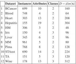
Table 1. Dataset Description.
Dataset Instances Attributes Classes D= dim(x) 1 BCancer 699 10 2 160 2 Blood 748 4 2 64 3 Heart 303 13 2 208 4 Hepatitis 155 19 2 304 5 HM 306 3 2 48 6 Iris 150 4 3 96 7 Liver 345 6 2 96 8 MM 961 5 2 80 9 Pima 768 8 2 128 10 STAust 690 14 2 224 11 TA 151 5 3 120 12 Wine 178 13 3 312
(HM), Iris, Liver Disorders (Liver), Mammographic Mass (MM), Pima Indians Dia-betes (Pima), Statlog Australian Credit Approval (STAust), Teaching Assistant Evalu-ation (TA), and Wine. These datasets are in the public domain and are available at the University of California at Irvine (UCI) Machine Learning Repository database [4]. The details of the dataset description and dimensionality are presented in Table 1. The di-mensionality D= dim(x) describes the number of elements of each individual required by PSOPRO-RVNS. Considering two prototypes for each class, and four parameters for each attribute S1, S2, d1, d2 are needed, the number of components of D for each
problem is 2× 4 × k × m, where k and m are the number of classes and attributes, re-spectively.
4.1 Parameters Settings
To apply PSOPRO-RVNS, the following factors are considered:
– The bounds for S1jh and S2jh vary between µjh− 6σjh andµjh+ 6σjh, where µjh
andσjh represent mean and standard deviation for each attribute in each class,
respectively;
– The bounds for d1
jhand d2jhvary in the range[0, 6σjh].
During the optimization phase, the parameters S1jh, S2
jh, d1jh, d2jhevolve within the
afore-mentioned boundaries. Also, the following technical factors are considered:
– The control parameters are set as follows:τ1= 2,τ2= 2 andϖ= 1.
– The size of population is fixed at 80; and the maximum iteration number (genmax)
4.2 Results and Analysis
The experimentation work is performed in two stages. First, PSOPRO-RVNS is applied to each dataset, where 10 independent runs are executed over each dataset. In each run, a stratified 10-fold cross-validation [25] is applied, where the percentage of correct classification for each fold is obtained, and then the average of classification accuracy is computed on all 10 folds. Second, to compare the performance of PSOPRO-RVNS against other well-known machine learning classifiers, similar experimental work is per-formed on the same dataset using Weka (the open source platform described in [25]). A stratified 10-fold cross-validation is also used to evaluate the performance of all classi-fiers.
The second stage of the experimental study includes the evaluation of PSOPRO-RVNS performance against other six machine learning techniques. These algorithms are chosen from different machine learning theories; they are: 1) Tree induction C4.5 (J48) [21], 2) statistical modelling, Naive Bayes (NB) [11], 3) Support Vector machines (SVM), SMO [19], 4) Neural Network (NN), multilayer perceptron (MLP) [23], 5) instance-based learning, IBk with k=3 [1], and 6) rule learning, PART [24]. The default settings in the Weka platform are used to run these tests.
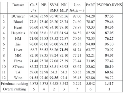
Table 2 documents the results of the classification accuracy obtained by PSOPRO-RVNS and the other algorithms based on testing dataset. The best results achieved on each application are marked in bold. PSOPRO-RVNS gives better results on 9 out of 12 datasets. Based on Demˇsar’s recommendation [12], the Friedman test is used in this work to recognize the rank of PSOPRO-RVNS among other classifiers. Based on the
Table 2. Experimental results based on classification accuracy (in %) to measure the performance of the different classifier compared with PSOPRO-RVNS.
Dataset C4.5 NB SVM NN k-nn PART PSOPRO-RVNS J48 SMO MLP Ibk, k = 3 1 BCancer 94.56 95.99 96.70 95.56 97.00 94.28 97.33 2 Blood 77.81 75.40 76.20 78.74 74.60 78.07 79.46 3 Heart 76.60 83.70 84.10 78.10 78.89 73.33 84.36 4 Hepatitis 80.00 85.81 83.87 81.94 84.52 82.58 87.05 5 HM 71.90 74.83 73.52 72.87 70.26 72.55 76.27 6 Iris 96.00 96.00 96.00 97.33 95.33 94.00 96.30 7 Liver 68.7 56.52 58.26 71.59 61.74 63.77 70.97 8 MM 82.10 78.35 79.24 82.10 77.21 82.21 84.07 9 Pima 71.48 75.78 77.08 75.39 73.44 73.05 77.42 10 STAust 85.22 77.25 85.51 84.93 83.62 83.62 86.10 11 TA 59.60 52.98 54.3 54.3 50.33 58.28 60.62 12 Wine 91.55 97.40 99.35 97.4 95.45 92.86 96.72 Friedman ranking 4.875 4.375 3.458 3.542 5.292 5.042 1.417 Overal ranking 5 4 2 3 7 6 1
classification accuracy in Table 2, the algorithms’ ranking results using Friedman test are shown on the last couple of rows in Table 2.
5
Conclusions
In this paper, a new methodology based on the metaheuristic algorithms PSO and RVNS is proposed for training the MCDA classification method PROAFTN. The pro-posed technique for solving classification problems is named PSOPRO-RVNS. During the learning stage, PSO and RVNS are utilized to induce the classification model for PROAFTN by inferring the best parameters from data with high classification accu-racy.
The performance of PSOPRO-RVNS applied to 12 classification dataset demon-strates that PSOPRO-RVNS outperforms the well-known classification methods PART, 3-nn, C4.5, NB, SVM, and NN. PROAFTN requires some parameters and uses fuzzy approach to assign objects to classes. As a result there is richer information, more flexi-bility, and therefore an improved chance of assigning objects to the preferred classes. In this study, using the metaheuristics PSO and RVNS to obtain these parameters proved to be a successful approach for training PROAFTN.
Regarding the execution time of PSOPRO-RVNS, it was noticed that, as expected, the execution time is dependent mainly on the problem size as this affects the num-ber of PROAFTN parameters (D) involved in the training process. Even though the number of PSO iterations was set to 500, PSOPRO-RVNS was able to generate the pre-sented results in significantly fewer iterations number (e.g., 100 iterations) with a very good speed. It is noticed that the execution time of PSOPRO-RVNS compares favorably with the execution time of NN in most cases. The remaining algorithms 3-NN, C4.5, NB, PART and SVM in declining order of speed were relatively faster than PSOPRO-RVNS. Nonetheless, the small penalty in computational time is only incurred off-line for PSOPRO-RVNS is less relevant when considering the time taken by PROAFTN to classify a new instance is virtually insignificant once it has been trained.
Acknowledgment
We gratefully acknowledge the support from NSERC’s Discovery Award (RGPIN293261-05) granted to Dr. Nabil Belacel.
References
1. D. Aha. Lazy learning. Dordrecht: Kluwer Academic Publishers, 1997.
2. F. Al-Obeidat, N. Belacel, P. Mahanti, and J. A. Carretero. Discretization techniques and genetic algorithm for learning the classification method proaftn. In Eighth Int. Conf. On
Machine Learning and Applications, pages 685–688, Los Alamitos, CA, USA, 2009.
3. E. Alpaydin. Introduction to machine learning. MIT Press, 2004.
4. A. Asuncion and D.J. Newman. UCI machine learning repository, 2007.
5. N. Belacel. Multicriteria Classification methods: Methodology and Medical Applications. PhD thesis, Free University of Brussels, Belgium, 1999.
6. N. Belacel. Multicriteria assignment method PROAFTN: methodology and medical applica-tion. European Journal of Operational Research, 125(1):175–183, 2000.
7. N. Belacel and M. Boulassel. Multicriteria fuzzy assignment method: A useful tool to assist medical diagnosis. Artificial Intelligence in Medicine, 21(1-3):201–207, 2001.
8. N. Belacel, H. Raval, and A. Punnen. Learning multicriteria fuzzy classification method PROAFTN from data. Computers and Operations Research, 34(7):1885–1898, 2007.
9. N. Belacel, P. Vincke, M. Scheiff, and M. Boulassel. Acute leukemia diagnosis aid using mul-ticriteria fuzzy assignment methodology. Computer Methods and Programs in Biomedicine, 64(2):145–151, 2001.
10. N. Belacel, Q. Wang, and R. Richard. Web-integration of PROAFTN methodology for acute leukemia diagnosis. Telemedicine Journal and e-Health, 11(6):652–659, 2005.
11. G. Cooper and E. Herskovits. A bayesian method for the induction of probabilistic networks from data. Machine Learning, 9(4):309–347, 1992.
12. J. Demˇsar. Statistical comparisons of classifiers over multiple data sets. Journal of Machine
Learning Research., 7:1–30, 2006.
13. R. Eberhart and J. Kennedy. Particle swarm optimization. In Proc. of the 1995 IEEE Int.
Conf. on Neural Networks, volume 4, pages 1942–1948, 1995.
14. N. E. Fenton and W. Wang. Risk and confidence analysis for fuzzy multicriteria decision making. Knowledge-Based Systems, 19(6):430–437, 2006.
15. P. Hansen and N. Mladenovic. Variable neighborhood search for the p-median. Location
Science, 5(4):207–226, 1997.
16. P. Hansen and N. Mladenovic. Variable neighborhood search: Principles and applications.
European Journal of Operational Research, 130(3):449–467, May 2001.
17. K. Jabeur and A. Guitouni. A generalized framework for concordance/discordance-based multi-criteria classification methods. In Information Fusion, 2007 10th International
Con-ference on, pages 1–8, July 2007.
18. J. Kennedy and R.C. Eberhart. Swarm intelligence. Morgan Kaufmann Pubs., 2001.
19. S. Pang, D. Kim, and S.Y. Bang. Face membership authentication using SVM classifica-tion tree generated by membership-based lle data particlassifica-tion. IEEE Transacclassifica-tions on Neural
Networks, 16(2):436–446, 2005.
20. R. Poli. Analysis of the publications on the applications of particle swarm optimisation.
Journal of Artificial Evolution and Applications, 8(2):1–10, 2008.
21. J. R. Quinlan. Improved use of continuous attributes in C4.5. Journal of Artificial
Intelli-gence Research, 4:77–90, 1996.
22. B. Roy. Multicriteria methodology for decision aiding. Kluwer Academic, 1996.
23. Y. Shirvany, M. Hayati, and R. Moradian. Multilayer perceptron neural networks with novel unsupervised training method for numerical solution of the partial differential equations.
Applied Soft Computing., 9(1):20–29, 2009.
24. D. K. Subramanian, V. S. Ananthanarayana, and M. Narasimha Murty. Knowledge-based as-sociation rule mining using and-or taxonomies. Knowledge-Based Syst., 16(1):37–45, 2003.
25. H. Witten. Data Mining: Practical Machine Learning Tools and Techniques. Morgan Kauf-mann Series in Data Management Systems, 2005.
26. C. Zopounidis and M. Doumpos. Multicriteria classification and sorting methods: A litera-ture review. European Journal of Operational Research, 138(2):229–246, 2002.