by
JOSEPH EDWARD WALL, JR.
B.S.E., Tulane University (1973)
S.M., Massachusetts Institute of Technology (1976)
E.E., Massachusetts Institute of Technology (1976)
SUBMITTED IN PARTIAL FULFILLMENT OF THE REQUIREMENTS FOR THE
DEGREE OF
DOCTOR OF PHILOSOPHY at the
MASSACHUSETTS INSTITUTE OF TECHNOLOGY August, 1978
Signature of Author...--r
Department of Electrical Engi<eeri g and Computer Science, August 11, 1978 Certified by... Certified by Thesis Superviso I,- - S ... ... ' I ? . - .' - . .. Thesis S4$rvisor 4A' Accepted by . ...
-2-CONTROL AND ESTIMATION FOR
LARGE-SCALE SYSTEMS HAVING SPATIAL SYMMETRY
by
JOSEPH EDWARD WALL, JR.
Submitted to the Department of Electrical Engineering and Computer Science on August 11, 1978, in partial fulfillment of the requirements for the Degree of Doctor of Philosophy.
ABSTRACT
Control and estimation problems for circulant and Toeplitz systems are studied using spatial transform techniques. In the finite-dimensional case, the discrete Fourier transform is used to provide a complete treat-ment of the system theoretic properties of circulant systems in terms of
lower dimensional, transformed subsystems. The centralized and decentral-ized control and estimation problems for circulant systems are approached
in the spatial frequency domain. Efficient off-line and on-line solutions to the optimal centralized problem are obtained. For the decentralized problem, suboptimal design procedures are proposed by analogy with the design of finite impulse response digital filters.
In the infinite-dimensional case, the z-transform is employed to solve the Toeplitz estimation problem. Motivated by recent work in the image processing field dealing with recursive estimation based on two-parameter models, the update step of a discrete-time Kalman filter for a Toeplitz system is shown to be equivalent to a smoothing problem. An investigation of the smoothing problem yields new insight into the two-filter smoother and yields formulas for sensitivity analysis and reduced order smoother analysis. This new two-filter smoother is then used to perform the filter update step for Toeplitz systems. Some implementation
issues of such a filter are then discussed. Finally, the control problem dual of the fixed-interval smoothing problem is posed and solved.
Spatial transformations play a crucial, fundamental role throughout this dissertation. The spatial frequency domain is found to be quite appealing when addressing control and estimation problems for spatially symmetric large-scale systems.
THESIS SUPERVISORS:
Professor Alan S. Willsky
Title: Associate Professor of Electrical Engineering Professor Nils R. Sandell, Jr.
ACKNOWLEDGEr4ENTS
I gratefully acknowledge the inestimable contribubtion of my two
thesis supervisors, Professor Alan S. Willsky and Professor Nils R. Sande-L,
Jr. Professor Willsky has provided constant enthusiasm and a continuous
stream of ideas for this work. The thoughtful and thought-provoking
com-ments and questions of Professor Sandell have contributed greatly to this
research. The friendship of these two men has also been important to me
as a graduate student at M.I.T., and is thankfully acknowledged.
The interest and suggestions of Dr. Alan J. Laub and Dr. David A.
Castanon, thesis readers, is also greatly appreciated.
The efforts of Ms. Barbara Peacock, Mrs. Evelyn Holmes and Ms. Fifa Monserrate in typing this manuscript have not been insignificant and are
sincerely appreciated. Thanks are also due to Mr. Arthur Giordani for his
excellent work and cooperation in preparing the figures in this document.
My parents. Joseph and Marjorie Wall, have steadily provided me with
generous amounts of advice, support, and encouragement, and I wish to take
this opportunity to express my deep thanks to them.
I also wish to thank my wife, Barbara, and my children, Joey and Susan, for their most special contribution to this research effort.
-4-DEDICATED
TO
/
TABLE OF CONTENTS
Page
No.
TITLE PAGE ABSTRACT ACKNOWLEDGEMENTS TABLE OF CONTENTS LIST OF FIGURES 1. INTRODUCTION1.1
Motivation
1.2
Summary
2. CIRCULANT SYSTEMS2.1
Introduction
to Circulant Systems
2.1.1
Definition
2.1.2 A Useful Spatial Transformation
2.2 Imbedding Tridiagonal Systems in Circulant Systems
2.2.1 Symmetric Tridiagonal Systems2.2.2 Antisymmetric Tridiagonal Systems
2.3
Examples
2.4 System
2.4.1
2.4.2
2.4.3
Theoretic ResultsControllability and Observability
Minimal RealizationsPole Allocation and State Reconstruction
2.5 Decomposition of Lyapunov and Riccati Equations
via the Spatial Transformation
2.6
Summary and Conclusions
3.
CONTROL AND ESTIMATION FOR CIRCULANT SYSTEMS
3.1 Centralized Control
3.2 Decentralized Control
3.2.1
Introduction
3.2.2
Optimal Decentralized Controller
3.2.3 Suboptimal Decentralized Controller
1
2
3
5
7
8
8
15
19
19
19
21
30
32
45
52
67
67
70
73
76
80
82
83
89
89
90
95
Table of Contents (continued) Page
No.
3.3 Computer Example: Circulant Control of a RectangularMembrane
ill
3.4 Circulant Control of Large-Scale Systems 117
3.5
The Dual
Filtering Problem
121
3.6
Summary and Discussion
125
4. THE FIXED-INTERVAL SMOOTHING PROBLEM 127
4.1
Introduction
127
4.2
Historical Review of the Two-Filter Smoother
134
4.3 A New Solution to the Fixed-Interval Smoothing Problem 1444.3.1 Motivation 144
4.3.2 Reversed-Time Markov Models 146
4.3.3 An Estimate Based on Future Observations Plus
A
Pioi
Information
149
4.3.4 The Solution
154
4.3.5 The Linear Time-Invariant Infinite-Lag Case 158
4.3.6 Discussion
161
4.4 Sensitivity Analysis and Reduced Order Smoothers
167
4.5 Conclusions
179
5. CONTROL AND ESTIMATION FOR TOEPLITZ SYSTEMS 183
5.1 Introduction to Toeplitz Systems 183
5.1.1
Definition
183
5.1.2 Optimal Control via z-Transforms 188
5.2 Attasi's Work in Image Processing 195
5.3 The Estimation Problem
202
5.3.1 Formulation and Solution
202
5.3.2
Implications for Filtering in Large-Scale Systems 213
5.3.3 Filter Implementation Issues 215
5.4 The Dual Control Problem 230
6. CONTRIBUTIONS AND SUGGESTIONS 242
APPENDIX A. CIRCULANT MATRICES 245
APPENDIX B. DISCRETE-TIME SMOOTHING FORMULAS 252
REFERENCES 259
LIST OF FIGURES
Figure Page
No. No.
2.1 The unforced dynamics of a circulant system 22 with three subsystems.
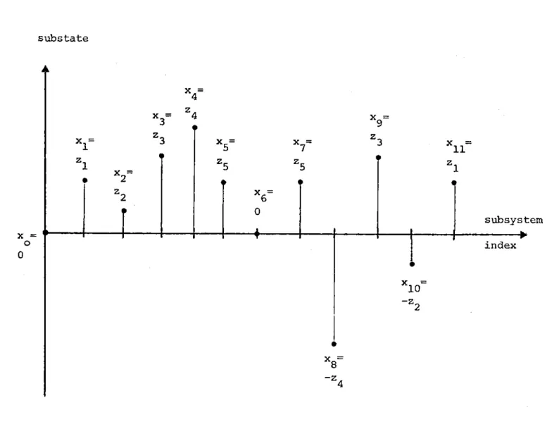
2.2 When a symmetric tridiagonal system is imbedded 35 in a circulant system, the initial state must
be extended in an odd way.
2.3 Imbedding an antisymmetric tridiagonal system 48 with an odd number of subsystems in a
circulant system.
2.4 Imbedding an antisymmetric tridiagonal system 53 with an even number of subsystems requires a
circulant system roughly four times as large.
2.5 Illustration of the classical vehicle traffic 54 loop.
2.6 A uniform longitudinal power system consisting 60 of N generators.
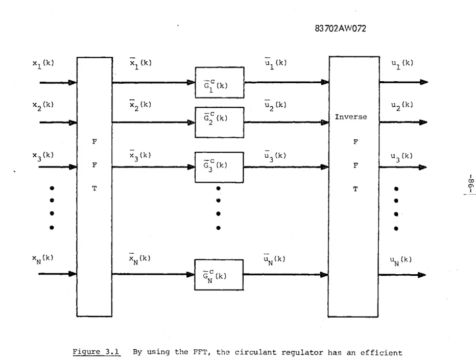
3.1 By using the
FFT,
the circulant regulator has 86 an efficient on-line implementation employingparallel processing.
5.1 Attasi's two step filtering procedure consists 199 of predicting ahead from line i-l to line i
and then smoothing along line i.
5.2 Each forward estimate uses exactly four 226 innovations and is obtained from a separate
Kalman filter.
5.3 A new forward Kalman filter is begun every 228 five subsystems, 'and at least four innovations
-8-CHAPTER 1
INTRODUCTION
1.1 Motivation
There has been a great deal of recent activity in the area of
large-scale systems [1]-[3]. These systems are found in such diverse
fields as power systems [4]-[6), transportation systems [7]-[9],
eco-nometric systems [10], [11], and packet switched data networks
[12]-[14]. For large-scale systems, the control and estimation problems
are often of such great complexity that the standard modern techniques
are computationally intractable. This intractability may be because of
either the on-line or off-line computational requirements. One concludes
that the adjective large as used in "large-scale systems" usually has the meaning of too large.
Various techniques have been proposed to reduce the computational
burden for control and estimation problems by exploiting special
struc-tural properties frequently found in large-scale systems. For example,
singular perturbation theory has been successfully employed to construct
simplified controllers and estimators for systems having multiple time
scales [15-[18]. Also, systems composed of weakly coupled subsystems
have been attacked by nonsingular perturbation theory to obtain
decentralized controllers [19], [20] or off-line computational savings
[21], [22]. Finally, there have been numerous approaches for determining
the stability of a large-scale system on the basis of the properties of
Decomposition and decentralization are two crucial elements in
large-scale system theory. Decentralization is directed toward the
reduction of on-line computational requirements and intersubsystem
communication. The price of the advantages, however, is often increased
off-line complexity. As pointed out in [23], other proposed benefits
of decentralization, such as increased reliability or increased
adap-tability, may be more imagined than real. The decomposition issue
concerns reducing the off-line computational burden associated with
obtaining a desired controller or estimator. A discussion of
decom-position vis-a-vis decentralization is found in [24].
It is often natural and useful to view a large-scale system as an
interconnection of much simpler subsystems. In many cases these
sub-systems are actually distinct physical entities, while in other cases
they are merely chosen for mathematical convenience, Decomposition
procedures are frequently based at the subsystem level. The nonsingular
perturbation decomposition and the stability tests for interconnected
systems, for instance, are based on a tearing of the system into
sub-systems which are usually distinct entities. The singular perturbation
methods, on the other hand, usually involve fast and slow subsystems
which are chosen on the basis of physical insight for mathematical
convenience. In the case of a decentralized controller or estimator,
the partitioning of inputs and outputs is also frequently done at the
subsystem level.
substantial activity in the image processing field.
The estimation of
discrete-space images from observations corrupted by additive noise
using techniques such as two-dimensional Wiener filtering result in
enormous computational burdens.
Thus one of the primary objectives of
work in this area is the discovery of computationally tractable
esti-mation formulas.
One approach toward the recursive estimation of
images has been motivated by the success of model based estimators
such as the Kalman filter
[253.
of interest here is the use of
two-dimensional models for the image process [26], [27].
Attasi [28) has considered least squares recursive estimation of
an image z(i,k) under noisy observations
y(1,k)= z(i,k)
+v(ik)
(1.1)
where the image is generated by the two-parameter model
x(i,k)
= Fx(i-l,k)
+ F x(ik-1) - F Fx(i-l,k-1)
+ w(i-lk-l)12
1
2
z(i,k)
H
x(i,k)
(1.2)
with the requirement F F
F2. The problem is to determine the
op-12
21l
timal estimate x(i,k) of x(i,k)
given the observations y(m,n) for
m
<
i and all n.
This estimate is shown to be obtained from a two
step procedure.
First a predicted value u(i,k) is computed from the
estimates x(i-1,n) for all n, as
(1-3)
ii(i,k)
=F
'ji-l,k).The error e(i,k) is now defined as e(i,k) = x(i,k) - i(i,k). Then the estimation problem is solved by
x(i,k) = x(i,k) +
e(i,k)
(1.4)where e(i,k) is the solution of the one-parameter smoothing problem
to estimate e(i,n), for all n, given y(i,n) for all n [28]. This
smoothing problem is solved by two Kalman filters, one moving in the
positive n direction and one in the negative n direction.
Two-parameter models such as Attasi's have had mixed success when
used for recursive estimation of images. Attasi's model will now be
considered in the context of large-scale systems.
Suppose that the vector quantity x(i,k) in Attasi's model is
interpreted as the state of subsystem k at time i. The term state is
used loosely here since the dynamics (1.2) are not standard state space
dynamics. Nevertheless, view Attasi's model as an infinite-dimensional
system propagating in time. His estimation problem, then, is just the
filtering problem for this infinite-dimensional system given
observa-tions up to the present. The update step of this filtering problem is
solved by one Kalman filter moving up the line of subsystems and one
Kalman filter moving down the line. The Kalman filter moving up the
line can be implemented by having each subsystem (say subsystem k)
perform a measurement update and then transmit this estimate to the
next (k+l) subsystem. Likewise, implementation of the Kalman filter
-12-and then communication of this estimate to the previous (k-1)
sub-system. This update procedure is not decentralized, but it is quite
efficient and interesting.
As discussed by Willsky [29], the proof of Attasi's estimation
algorithm employs a bilateral z-transform along the k direction and
treats the i direction as the time variable. In terms of the
inter-pretation of the model as an infinite-dimensional system, this
cor-responds to taking a z-transform with respect to subsystem index
(essentially a spatial z-transform). In this manner, Attasi obtains independent subproblems indexed by the variable z. That is to say, this problem is very nicely decomposed by the z-transform.
The same approach of taking spatial z-transforms has also been used to address control problems for infinite-dimensional
one-parameter systems of the form
+Mo
x(i,j) =
Z
A x(i-l,k) + B u(i-l,k) (1.5)k=
j-k
j-k
k=-00
Melzer and Kuo [30] design optimal centralized regulators in this
manner for spatially invariant quadratic cost functions. Optimal
cons-trained decentralized regulators for the same class of cost functions
are similarly designed by Chu [31]. The important result, at least in
the centralized case, is that the optimal control problem decomposes
into a set of optimal control problems of dimension equal to the
In both the estimation problem of Attasi and the control problems
of Melzer and Kuo and of Chu, the key step is the use of the spatial
z-transform to decompose the problem. It is possible to use the
z-transform in these cases because the systems are spatially invariant,
i.e. all the subsystems are identical and the influence of subsystem
k on subsystem depends on only k-Z. The objective of this thesis is
to examine in depth large-scale systems possessing the structural
pro-perty of spatial symmetry. Specifically, the control and estimation
problems for infinite-dimensional Toeplitz systems [see (1.5)] and their
finite-dimensional analog are studied. Such finite-dimensional systems
are called circulant systems. In the case of circulant systems, the
discrete Fourier transform will be found to be the analog of the
z-transform
used for Toeplitz systems.The spatially symmetric systems studied in this thesis are
obviously an extremely special type of large-scale system. The purpose
in studying such a special class of systems is to determine just how
far one can go in exploiting spatial symmetry to obtain efficient
on-line implementations of controllers and estimators, or separating a
large problem into more tractable subproblems. The issue of decentra-lization and decomposition, therefore, are crucial throughout the thesis. Also, for spatially invariant systems one can study such phenomena as
the spatial propagation of disturbances which are obviously present
-14-There has apparently been only very limited work done on circulant
systems. Dickerson and Erickson [32] have obtained some weak stability
results concerning circulant systems, and these are analyzed in the
sequel. Some areas where circulant matrices have been used include
the study of certain binary codes [33], [34], the generation of Markov
chains used as digital signals [35], the generalization of Clarke
com-ponents for polyphase networks [36], and the spherical model of a
ferromagnet [37]. Circulant matrices have had extensive use in the
field of digital image processing [38]-[40].
Let the image radiant energy at the point (x,y) be represented as
g(x,y) and the object radiant energy as f(x,y). Then the image and
object distributions are modelled as obeying an integral equation
in-volving the point spread function h as follows:
g(xy) =
fh(x,
y, u,v, f (u, v) ) dudv (1.6)By making the simplifying assumptions that
(i) h acts as a scalar multiplier, i.e, h(x,y,u,v,f(u,v)) = h(x,y,u,v)f(u,v)
(ii) h is spatially invariant, i.e. h(x,y,u,v)= h(x-uiy-v)
one reduces (1.6) to the two-dimensional convolution
g(x,y)
f
f
h (x-u, y-v) f (u,v) dudv (1.7)The image restoration problem is to estimate f from possibly noisy
mea-surements of g. One digital approach to this problem is to sample g at
points on a rectangular grid and then form a vector g. by
lexicographi-cally ordering these samples. A vector f. is similarly obtained from f
and the relationship expressed by (1.7) may be approximated as
g.
= Hf.
(1.8)i T
i
where the matrix H is block Toeplitz with Toeplitz blocks [40]. By
T
using a circulant approximation HC to HT, effective and computationally
tractable algorithms for the inversion of (1.8) have been obtained [38],
[39]. The key to these algorithms is the use of the fast Fourier
Trans-form to diagonalize circulant matrices. This same diagonalization
procedure is used heavily in the sequel to study circulant systems.
1.2 Summary
Chapter 2 introduces circulant systems and develops many of their
properties. Circulant systems are linear systems defined in terms of
(block) circulant matrices. Such matrices are discussed in Appendix A
where it is shown that the eigenvectorsof a circulant matrix are fixed
by its dimension. This property is then used to develop the diagonalizing
property of the discrete Fourier transform. Using this transformation,
various' system theoretic results are obtained for circulant systems, and
circulant Riccati and Lyapunov are efficiently decomposed. Chapter 2
-16-be im-16-bedded in circulant systems roughly two or four times as
large. Further, examples of circulant systems and tridiagonal systems
that can be imbedded in circulant systems are given.
The control and estimation problems for circulant systems are
the subject of Chapter 3. For the most part, Chapter 3 deals directly
with the control problem; the estimation problem is treated by duality
in Section 3.5. The centralized linear-quadratic control problem is
shown to (i) decompose into low order control problems and (ii) have
an efficient on-line implementation employing parallel processing.
Both these results are obtained by using the spatial transformation
introduced in Chapter 2. The fixed structure decentralized control
problem is treated in Section 3.2. Necessary conditions for the
op-timal decentralized gains are obtained but are not found to decompose.
Suboptimal decentralized controllers are then proposed by considering
the analogous situation of the design of finite impulse response
di-gital filters. Various digital filter design techniques are discussed
for designing decentralized control gains. A computer example of
cir-culant control for a rectangular membrane is also included. The
pos-sibility of using a circulant control law for a general large-scale
system is examined in Section 3.4. Throughout Chapter 3 an attempt
is made to use the spatial transfonnconcepts to obtain centralized
and decentralized controllers. That this goes much further than just
using transforms to decompose the centralized problem can be clearly
viewpoint is essential for understanding the suboptimal decentralized
control laws that are presented.
It has been stated that the update step for Attasi's estimation
problem is equivalent to a smoothing problem. This statement will be
generalized in Chapter 5. The purpose of Chapter 4, however, is to
carefully study the fixed-interval smoothing problem. In particular,
the Mayne-Fraser two-filter smoother is studied here. Section 4.2
presents an historical review of the two-filter smoother, discussing
the work of Mayne [413, Fraser [42], and Mehra [43]. By using
reversed-time Markov models,
4
new solution to the fixed-interval smoothing
problem is obtained which clearly demonstrates the use of (i) apriori data, (ii) past measurements, and (iii) future measurements in
computing the smoothed estimate. Using this new solution, a sensitivity
analysis and an analysis of reduced order smoothers are performed. Also,
using the insight gained in this approach, a new change of initial
con-ditions formula for the smoothed estimate is obtained.
Chapter 5 deals with the control and estimation problems for
infinite-dimensional Toeplitz systems. The view here is to consider
explicitly the filtering problem and then treat the optimal control
problem by duality in Section 5.4. After defining Toeplitz systems,
the work of Melzer and Kuo [30] and Chu [31] on optimal control of
Toeplitz systems is reviewed. Attasi's [28] estimation problem is
then considered, and the model (1.2) is shown to correspond to a
-18-for general Toeplitz systems is then treated.
It is shown that the
update step in this case is equivalent to a smoothing problem along the
subsystems.
Finite-dimensional realizations of the update operation
are presented and the implications of these realizations for filtering
in large-scale systems are discussed.
Also, some filter implementation
issues are examined.
Chapter 5 tries to give a cohesive treatment of
Toeplitz systems and the associated control and estimation problems
by employing a spatial z-transform.
This treatment is much deeper than
that of Melzer and Kuo or Chu in that the spatial transform is not
merely used for decomposition purposes.
Rather, the spatial frequency
domain provides the necessary insight for the proposed filters and
controllers in Chapter 5.
In conclusion, Chapter 6 presents the contributions of this thesis
and suggestions for future research.
In listing the contributions
of this work, a summary of the thesis is also provided.
CHAPTER 2
CIRCULANT SYSTEMS
2.1 Introduction to Circulant Systems
2.1.1 Definition
A circulant matrix is a square NXN matrix in which each row is a
circular right shift of the row directly above it, i.e. a matrix of the
form
a0
-JaN-2... a
a a0 aN-l... a2 A= (2.1) a a a ... a2
1
0
3
aN-1
aN-2
aN-3. 0.aThe right shift of each row is called a circular shift because the
ele-ment that is shifted out on the right side re-enters the matrix on the
left. Block circulant matrices are defined similarly, with the elements ak being replaced by submatrices Ak. A matrix is called block circulant of order N if it can be partitioned into N2 blocks A such that the re-sulting structure is the same as (2.1).
Deterministic continuous-time circulant systems are defined in terms
of block circulant matrices as follows: the state of a circulant system
-20-(2.2) x(t) = A x(t) + B u(t)
and the output is given by
y(t) = C
x(t)
(2.3)
where
x(t)
e
3Rnt
is the state vectoru(t)
e
3R
is the input vectory(t)
e
xtN is the output vectornNXnN
A S IR is a block circulant matrix of order N
B
e
3R is a block circulant matrix of order NC
G
]RpNxnN
is a .block circulant matrix of order NThis circulant system is
just
a finite-dimensional linear system forwhich the system, input, and output matrices are all block circulant.
Discrete-time circulant systems are similarly defined.
The state x(t) of a circulant system may be viewed as consisting of
N substates xk(t) R n, k=0, l,.. .,N-1, according to the partition
x(t)
=x
0(t)
x
(t)
x
(t)
x-(t)
(2.4)
(2.3) may be written in component form as
N-1
x (t) = E Ax
. (t) + B. u (t) (2.5)dt
k
.i
(k-i)mod N
i
(k-i)mod N
N-1
y (t) =>C
3y.
(t)(2)
k
= t E(k-i)mod N(2.6)
i=o
where the notation (k-i)mod N is used to denote the unique integer
j
inthe set {O,,. ... ,N-1 such that (k-i)+j is divisible by N. Figure 2.1
illustrates the unforced dynamics of a circulant system. All of the
subsystems are identical in the sense that each substate xk(t) has
* the same self-dynamics A
0
* for any i. the same interaction with substate x (k.)d N (t).
Also, for any i, the subinput u(k+i) d N(t) affects each x.(t) in the same way, and each xk (t) contributes equally to the suboutput
yk+i)mod N t). Thus circulant systems may be called spatially symmetric where spatial refers to the subsystem index number. One way to view
this is that someone located at subsystem k looking out at the rest of
the subsystem, observes behavior that is independent of k.
2.1.2 A Useful Spatial Transformation
-22-83702AW073
A
0
0A
A
1withtthtsubsystem
s
A A AA
sitbsysrem 2ussbsysmsmfixed eigenvectors given by
k
N w2k N W (N-1)kN
, k=O,1,...,N-1(2.7)
where W
ex(
-i.Since the N values W
,k=0,1...,N-l, are all
NN
N'
..
Nl
r
l
distinct, the eigenvectors
4k form a linearly independent set, and so
any circulant matrix can be diagonalized.
If 0 is the matrix of
eigen-vectors,
O
1
2
then 4
A Vis diagonal, i.e.
A =
A
@
N-l I I21Q
(2.8)
(2.9)
I I
-24-It is easily shown
[
44] that the eigenvalues
Xk
of A may be computed
from
N-1
Ak
.Z
aWk
(2.10)
i=oiN
This equation means that the finite sequences
(A
0' l
1,
'., -
1)
and
(aO1a
1,...,aN-l) are related by the discrete Fourier transform (DFT).
Thus the eigenvalues of a circulant matrix can be obtained by applying
the fast Fourier transform (FFT) algorithm to the top row of the matrix.
Consider now a block circulant matrix A where the blocks
A
have
dimensions rxs.
In analogy with the circulant case, the partitioned
matrix (D
is
defined as
r
I -I
e00
r
r
w
w
2
W IWI
... N r Nr2
4
W I
WI
N r N r N-1 2 (N-1) W I W I-N
r
Nr
rWN-lI
N
r
2(N-1)
W
I
N
r
(N-1) (N-i) WI N:where Ir is the rxr identity matrix.
In Appendix A it is shown that
-
-l
A r AS
yo'lC A 2 , N.N-l
K)
(2.12)I
r
I
I
r
I
r
I
r
(2.11)
where the blocks Ak on the diagonal are rxs matrices satisfying
N-1
A =
A.
W (2.13)j=o
That is, in the block circulant case, the elements of the block diagonal
form are the DFT of the top block row of the block circulant matrix.
A very useful change of basis can. now be defined for circulant
sys-tems. Let
x(t)
= nx(t)
(2.14)n
-1
u(t) = Du(t)
(2.15) y(t) = 0 y(t) (2.16)p
It is to be noted that n x(t) = x(t) or, in component form,
n
N-1
- ki x (t) = x.(t) W (2.17)k
i
I
N
1=0i.e. the substates
{x(t)}
are the inverse DFT of the{ykt).
Thus,the substates {x (t), subinputs {w (t)}, and suboutputs
Iyk
(t)} are simply the respective DFT's of{x
(t)}, {uk(t)}, and{yk(t)}
where the transform is taken with respect to the index k. The
trans-formed system is described by
x(t) =
(4-
A(nx(t)
+(
B
0)n)(t)-26-y(t)
= ~C1Cn)x(t)
= C x(t) (2.19)
where A, B, C are block diagonal matrices whose elements are given by
(2.13).
Under this change of basis, the system is composed of N completely
independent complex-valued subsystems
ftxk (t) = Ak xk(k) + Bkuk(t) (2.20)
Yk(t)
= Ckxk(t)
, k=0,l,...,N-1 (2.21)This independence is in the "frequency domain", however, and is not
directly applicable to decentralized control or estimation problems
since each transformed subsystem xk1(t) depends on all of the subsystems
x. (t), i=0,l,...,N-l. Computation of the transition matrix, on the
other hand, has been decomposed into the computation of the N lower
dimensional transition matrices of the Ak. Since the change of basis in (2.14)-(2.16) and the determination of Ak' k, and Ck are easily done using the FFT, the dynamic behavior of a circulant system is much
easier to determine than that of a general nN-dimensional system.
In order to gain further insight as to why the transformed dynamics are uncoupled, consider the dynamics of the kth substate,
N-1
dx(t) A. x (t) + B. u (t) (2.5)
Notice that each of the two terms on the RHS of (2.5) is a circular
con-volution sum. Because of the relationship between convolution and Fourier
transformation, one expects (2.5) to be decoupled in the frequency domain. --kt
This result is obtained by multiplying (2.19) by W and summing over k,
N
N-1d
()-k?.
---
xk
(t)
WN
N-1N-1
-kZak
9
=ZZ
A.x
mo
dt)
Wk +j
u .
t) W
k=o i=o0
x
(k-i)
WN
+
Biu(k-i)
mod
4
N
N-1
N-i
E
A.W x ) t)W+-k) SN(k-i) mod
NNi=0
k=o
N-1
N-1
Z Bi
}
>7(
w (i-k)9 .N
(k-i) mod
N
N
i=0
k=o
(2.22)
But (2.22) is just an expanded version of
-x jt) = Ax(t) + Bzuz(t)
(2.18)
The key element here is the fact that a circulant matrix times a vector
equals the circular convolution of the top row of the matrix with the
vector.
The Fourier transform is then applied to convert convolution
into "multiplication in the spatial frequency domain".
Before concluding this discussion of the spatial transformation,
several identities will be presented here for easy reference throughout
the chapter.
Consider first a real block circulant matrix A and the
-28-N-1
Re[ = ReZ AWN-ki
i=0
N-1
= 1A. Re1--ki j=oN-1
= A. Re W(N-k)1i .1
N j=0 = Re[N-k (2.23)Similarly,
N-1
Im[Ak
= Im A.
i]
N-1
=-rm ZA.W
(N-k)i 1=0 =-Im
k l
(2.24)Equations (2.23) and (2.24) just state the well-known property of the DFT that real-valued sequences have transforms with real parts that are even
and imaginary parts that are odd. The sequence {Re[AJ} is called even
because Re [Ak] = Re[Ak] where the indices are modulo N. The sequence {Im[Ak} is odd since Im[A] = -Im[Ak]. Next,. identities for a symmetric block circulant matrix
Q
will be obtained. The symmetry ofQ
isequiva-lent to the following condition on the blocks Qk:
(2.25)
Therefore,
N-1
ReEWN-ki i=o. [N-1
S (-i)modN
N-1
Q
Re[WN-kg] k=o k I Re Wki N , =(-i)mod
N =Re[Qk]
(2.26)
Similarly,
N-1
IQ1Q =Q'
ImiW Ikm Q (-i)mod N NN=i
N-1 =-Q Im W-kk(2.27)
Combining (2.23) and (2.26) for the real part of
Q
and (2.24) and (2.27)
for the imaginary part of Qk yields
Re [k
=Re[Q-k1
Im
k=
Im -k](2.28)
(2.29)
The final identity relates the transforms of A and A'. If A is a block
circulant matrix and B=A', then B is also block circulant. Partitioning
Re
%
I
I I
-30-B according to
(2.1), bl
N-1
ReBkl=
B.i=O
N-1
=AtN-i
i=O.N-1
=AtY=O
=Re A
1J
Also,
ock
B equals A'k. Thusk N-ko
-ki
Re W k [N Re W ki-k Re
N
Re
1
k
(2.30)
N-1Im
B
A'Ims=
-ki
.N-k
Ni=O
N-1
=-E A' Im W-kk k=O k [=
-Im
kl
(2.31)
Combining (2.30) and (2.31) yields
(A') =
(2.32)
where * denotes Hermitian, i.e. the transposed complex conjugate. These
identities will be heavily used in Sections 2.4 and 2.5.
2.2
Imbedding
Tridiagonal Systems in Circulant SystemsThe usefulness of circulant models is increased by showing how
systems. Symmetric tridiagonal systems are linear systems for which
the system matrix is block tridiagonal and the blocks on the subdiagonal
and superdiagonal are equal. For antisymmetric tridiagonal systems, the
blocks on the subdiagonal are the negative of the blocks on the
super-diagonal. Brockett and Willems [ 45
]
have shown how a symmetric tridiag-onal system could be imbedded in a circulant system roughly twice aslarge. The imbedding of an antisymmetric tridiagonal system is new, but
strongly motivated by Brockett and Willems.
Before presenting the imbedding methods, it is interesting to con-sider why one would desire an imbedding of this type. One reason might be the computational advantages associated with determining the
eigen-values or solving a Riccati equation (see Section 2.5) for a circulant
system. The work of Jain and Angel [26
1,
however, suggests that similarsavings can arise from a direct analysis of these tridiagonal systems. It
is in the area of decentralized control and estimation that the
motiva-tion for this imbedding is found. Consider a decentralized control
structure where feedback is allowed not just from the nearest neighbors
but from the first and second nearest neighbor on each side. The
re-sulting closed loop system matrix is no longer tridiagonal - it is still
circulant if the system has been imbedded in a circulant system. This is
because, as is shown in Appendix A, the product or sum of circulant
ma-trices is still circulant. Therefore, since feedback can destroy the
tridiagonal property but not the circulant property, it is useful to
-32-2.2.1 Symmetric Tridiagonal Systems
The unforced symmetric tridiagonal system under consideration is
given by
d
z (t) =F Z (t) F F z (t)0
11
F F F Jz2
(t) F *1
F
F F z(t) (2.33)~1II~1
0
N
(.3
nN
where z(t)
eR
. This system is close to being circulant; all that isneeded is for the upper right hand corner block and the lower left hand
corner block of F to be F1 instead of zero. What this means physically is
that the symmetric tridiagonal system fails to be circulant because the
two end subsystems do not directly interact with each other.
The system (2.33) is imbedded in the following circulant system of
dimension 2n(N+l):
d
x (t) =A x (t)F
F
F
x0
(t)
F F F x (t)1
0
1
F
. 0 FF
F1F0
2N+ (t) (2.34)The idea here is for x1(t),...,xN (t) to equal z1(t),...,z N (t),
respec-tively, for all time t. In order for x1(t) to equal z1(t), it is
neces-sary that
d
d
-x (t) =-z Ct) (2.35)dt
1X
dt 1
F
x
(t) + F
x
(t) + Fx2(t)
=Fz(t)
+F
z2(t)
1
0(t
0x
11 2
0 1
1 2
Equation (2.35) implies that x0(t) must be identically zero. Demanding
that x (t) equal z (t) implies, by the same argument, that x (t) must
N
N
N+1
also be identically zero. Now the question becomes how can x
Ct)
andxN+jt) be made to remain at zero? For x+l(t) to be identically zero, it derivative must also be zero for all t,
d
r-xl
(t)
=F
X
(t)
+ Fx
Mt)
+ FX
(tI (2.36)dt
N+l
1
N
ON+l
1 N+2
=
F xN(t)
+ x(t)l (since xN+l(t)=0)-0
Clearly a sufficient condition is xN+2(t) = -xN(t) = -zN(t) for all t.
That is, if xN and 2N+2 exert equal but opposite "forces" on xN+l' then
+1 will remain at zero. Similarly, for x0 to remain at zero it suffices
to have x
2N+
t)
= -x1(t) = -z(t)
for all t. Continuing this line ofreasoning for N+2, XN+3, .-. and
x2N+l' X2N,yields the conclusion
-34-x (o) =
0
(2.37)0
xk(o) =zk(o)
xN+Il(o)
0
x
(o)
=-z Co)
,k=l,2
...N
2N+2-k
k(
'
then for all time t, the substates x0 (t) and xN+l(t) remain fixed at zero and zk(t) =
Xk(t)
= -x2N+2-k(t), k=1,2,...,N. This extension isillustrated in Figure 2.2 for an example with scalar subsystems. In
this manner, a symmetric tridiagonal system can be imbedded in a
circu-lant system.
This imbedding procedure is analogous to a method used to determine
the transverse displacement of a finite string
[
463.
The displacementof a string having fixed ends at 0 and L is given by the one-dimensional
wave equation. In the case of an infinite string, the solution of the
wave equation is the well known d'Alembert solution. The displacement
of the finite string can be obtained from the infinite string analysis
by means of the following procedure. The initial displacement of the
finite string is extended to an odd periodic function of period 2L. The
initial velocity is also extended in the same way. The resulting
dis-placement between 0 and L of an infinite string having these extended
initial displacement and velocity is identical to the displacement of
the finite string. Thus the behavior of a finite string can be obtained
substate
A
X,=1
Zjiz
X2Z2
x3 Z-z
39
:i
2
3
4
z
45
z5
'4 56
0
7
8
9
10
11
a - -a-61 XT-- 5
x10 -z2subsystem
index
-9
-z
3 X8 -z4Figure 2.2 When a symmetric tridiagonal1 system is imbedded in a circulant system, the initial state must be extended in an odd manner.
x =0
0
L
-
-36-periodic extension of the initial displacement and velocity is essentially
the same procedure as the imbedding formula (2.37).
The idea of this imbedding procedure is also somewhat similar to
the idea behind the method of images used in electrostatics. The method.
of images can be used, for example, to solve the problem of a point charge
q placed near a perfect conducting plane of infinite extent. The method
replaces the conducting plane with a point charge -q located at the mirror
image of charge q. The potential of these two charges is zero where the
conducting plane was located. In the case of imbedding a symmetric
tri-diagonal system in a circulant system, the substates x0Mt) and xN+l(t)
are identically zero. The mirror image of the state z(t) (see (2.37)) is
used to ensure that these two subsystems remain at zero.
The case of the tridiagonal system with scalar subsystems, i.e. n=l,
will be studied further. First, a nonsymmetric tridiagonal matrix
0
N-1
f
f
f
0
1
0
N.J
F =1
0
(2.38)*
f
N-
i
f
f0
1 0
can be transformed into a symmetric tridiagonal matrix by a similarity
N-1
1
2
(fN-1
1
2
0
N-1
(f
1/f1
-t Fthen PFP
IS symmetric,
f
0
1 N-i
f N- f0 f fN-i
0
1
N-1
0
1 N-i
0
0
f1N
1 N-2if
f
f
Hence the assumption that F = F' can be made without loss of generality.
Next the eigenvalues and eigenvectors of the symmetric tridiagonal
matrix F will be found from the eigenvalues and eigenvectors of a
circu-lant. Let A be the 2(N+i) x2(N+i) circulant matrix obtained from F
N 2(N+l)
according to (2.34). The linear transformation S : R -+ R is
de-fined componentwise as follows:
I
1
(2.39)-l
PFP
=1
(2.40)
-38-0,
k=O
or
N+l
(SW)=
w
, k=l,2,...,N (2.41)-W2N+2-k ' k=N+2,...,2N+1
N
where w e3R . Clearly S is just the linear transformation used to imbed
a tridiagonal system within a circulant system, i.e. x(o) = S z(o). For
N
any vector w
6
R , it is trivially verified thatSFw= A
S
w (2.42)The equation SF = AS is the aggregation equation that arises in large-scale system analysis when an aggregated model is being constructed. In
the context of aggregation, the state z is the state of a large-scale
system, and F is the corresponding system matrix. The transformation S maps z into an aggregated state x = Sz where the system matrix for x is A and must satisfy the aggregation equation. It is well-known that the
eigenvalues of the aggregated system matrix are a subset of the
eigen-values of the large-scale system matrix. In the context of imbedding
a tridiagonal system within a circulant system, the equation SF=FA can
be thought of a a "disaggregation" equation since the resulting state is
of higher order than the state of the original model.
If w is an eigenvector of F corresponding to eigenvalue
X,
thenHence
X
is also an eigenvalue of A with eignevector S w. What are theth
eigenvalues of A? From (2.10), the k
eigenvalue
isS=f
k 0+
f
1W
2N+2f
1W
2N+2f + 2f cos ,
k=0,lr...,2N+l
(2.44)0
1
\N+l
Thus there are only N+2 distinct eigenvalues -- eigenvalues
X 0
f0 + 2f andA
f
- 2f are not repeated; the otherN eigenvalues
occur twice.1+1
0
1
Can
A0
also be an eigenvalue of F? Since the corresponding eigenvectoris
1 (2.45)
and c0 is obviously not in the range space of
s, X
cannot be an eigen-value of F. Similarly, eigenvalueXN+
Of A has eigenvector+1
-l
= (2.46)N+l
+1
-1
and, since N+1 cannot be in the range space of
S,
XN+1
is not an eigen-value of F. The only remaining candidates for eigenvalues of F are the-40-repeated eigenvalues of A.
Consider the pair of eigenvalues
Xk
and
X2N+2-k*
Any eigenvector Xk of A corresponding to this eigenvalue
can
be written as a linear combination of the eigenvectors ck and
42N+2-k'
k/20020k
Cos k2Trj
sin k2Tr (N+l/
- l Csk (N+l1 j .i. k (N+l) IT cos FN+ r -j
sin(
+
l cosk (2N+)Tr)
. k (2N+1) T)co(
N+l snN+1
Cos(I + COS N + k (N+1)7
cos
N+1)+
(k (2N+l) Tr\N+l
j
sin
sin(
14+ .i. k (N+I) 7 ( i N+l . i . k ( 2N+1Tj
sin(iN+)
(2.47)(a+S)
(C+s) cos(0,+0)
S
2k(a+f)
CoskTr)
(a-f)
cos
k(2N+1)Tr)+
j
(-)
Xk =a
+
j
(S-t)
+
j
(5-a)
+
j
(S-t)
sin(-j)
sin
sin kT)Si
k (2N1)Tr
For Xk to be in the range of S requires, from (2.41) , that the 0 th and
th
the (N+l)
components
of Xkbe
zero, i.e. (c+6) =0
and (a+ )cos(kr) =0.
Therefore, choosing
a
=-s
yields an eigenvector ik of F, i.e.Xk.=sTk (2.48)
A purely real eigenvector is obtained by letting
a/
= - =2sini--\N+l,
S/2kwT\sin
i--k= sin+l,(2.49)
k.
.2kNTr
sin(N+components 1 through N of Xk. The corresponding eigenvalue of kis
Xk
= f + 2f1 cos(---.From the above analysis, it is clear that the eigenvalues of a
sym-metric tridiagonal (finite) Toeplitz matrix can be found using the FFT
algorithm. This is. proved more directly in [ 26 ] by Jain and Angel. Using the DFT to efficiently diagonalize symmetric tridiagonal matrices,
Jain and Angel are able to decompose the vector filtering equations
arising in the restoration of images into a set of uncoupled scalar
fil-tering equations. This is completely analogous to the decomposition of
Lyapunov and Riccati equations in Section 2.5. In fact, their results
on efficient algorithms for image processing were one of the motivating
-42-Finally, it is noted that the idea of imbedding a symmetric
tri-diagonal system within a circulant system can be extended to higher
di-mensions.
Consider a tridiagonal system
z
(t) F F z1(t}1
0
11
dz2(t)
F
FO
z2(t)
d
2
1
0
*02(2.50)
dt
.* F zN(t) F1 F0 0 zN(t)where each substate
zk(t)
is itself composed of q
sub-substates,
zkl(t)
zk(t)
=zk
2(t)
, k=l,2,...,N(2.51)
zkg(t)
and the matrices F0 and F have the special forms
00
F01 F00
F
OF0(2.52)
0
F . F01F1 0
Fb2
10
1,
(2.53)
0~F
10Since the individual subsystems are symmetric tridiagonal systems, the
imbedding procedure can be applied at the subsystem level to yield
x(t) A A1x(t
x2
AA
.x(t)
xdt)
1
0
*2dt
-(2.54)
. .0 AA1
xN (t) A1 A0N
(t)where the substates x(t) are composed of (2q+2) sub-substates, xk(t)
=
Szk(t)
and
F
F
F
00
01
01
F01
F00
F01
A0
F
01F
0 0F
(2.55)
F
0 1F01
F01
F00
-44--F
Q
10
A = (2.56)
10
For this imbedding to be valid, it is necessary that xk,0(t) and x (t) be identically zero. Writing out (2.54) for xk,(t) ,
d
dt 0
(t)
= F1 0 -1,0 (t) + F01 ,2q+2(t)
+ F00 ,0(t)++ F
0 1,l(t) + F
1 0\+1,
0(2.57)
A consistent solution is obtained if x-1,0(t), x 0 (t) , xk+,0o(t) are
all zero and Xk 1(t) = - ,2q+2 (t). Similarly, one sees that all the
,q+l(t) are identically zero, and so this imbedding is valid. The re-sulting system (2.54), moreover, is itself a symmetric tridiagonal system.
Applying
the imbedding procedure to it
yields
x (t) A A1
A
1x(t)
0
C)1
0
x1(t)
A1
A
A1 0
"x1(t)
d- (2.58) dt . . * A .5.
,
1
2N+2 (t) A 10
2N+2a circulant system where the h Locks of the system matrix are themselves
in a circulant system of order 4n (q+1) (N+1). In Section 2.3, an example
of such a symmetric tridiagonal system will be described.
2.2.2 Antisymmetric Tridiagonal Systems
An unforced antisymmetric tridiagonal system has the form
a
-z(t)
=F
z(t)
dtF
-F
zM(t)
0 1 F F -F z2(t)1
0
1
2
=F- (2.59) .- F.
1
F Fz(t)
1
0
N
nN
where z(t) eaR . It will be shown that there are two different imbedding procedures for antisymmetric tridiagonal systems depending on whether N,
the number of subsystems, is even or odd. For odd
N,
the propercircu-lant system has order 2n (N+1), just as in the symmetric tridiag-
onal
case. For even N, however, a circulant system of order 4n(N+l) is necessary.The situation when N is odd will be considered first. The candidate
-46-d
x(t) = A x(t) F0 -F1(I
F1 x0(t)F1
F
-F
x1(t)
F -1 (2.60) -F1 F F0 2N+1(tThis circulant system is very similar to the circulant system (2.34) used
for imbedding symmetric tridiagonal systems. Just as in the symmetric
case,
the substates x 1(t)
,ree,xN(t) equalzl(t)
,. ,zN(t) , respectively, for all time. This immediately implies that x0 (t) and x N+1t) must beidentically zero. Since xN+1(t) is zero,
d
+t=Fx
t(t)=F(t)t-) (2.61)JE
N+l
1 N
F
0xN+jt)
1xN+
2t
= F1[x(t) - x2(t)l (since xN+(t) 0)
-0
A sufficient condition here is that xN+2(t) = xN(t) = zN(t)', in contrast to the symmetric case. Once again, XN and
x+
2 exert equal but oppositeforces on XN+1, but in the antisymmetric case this requires XN+2(t)=xN(t).
Examination of the derivative of x (t) quickly leads to the conclusion 0
differ-ence between the symmetric and antisymmetric cases, the argument will be
continued for 'N+2(t) and x2N+1(t). The requirement is that xN+2 (t)=xN (t); hence
d
d
d 2(t) =. xW(t) (2.62) FxN+j(t)
+ F0XN+2
(t) - F1 XN+3 (t) =FxNj(t) + F0 XN(t) - F +1t) F0 xN+2(t) - F1 xN+3 ( t) =F (t) + Fx
(t) (sincexN+
1(t) =0)
Requiring
N+
3(t) = -xN-Ct) = -zN-1(t) obviously suffices. The condition X2Nt)
=-x
2(t) = -z2 t) is obtained similarly by considering x2N+1 (t).Continuing this argument leads to the conclusion that if
x(o) =
0(2.63)
xk(o)
=zk+l
x2N+2-k (o) =
(-)
zk o)
k=1,2
,...,Nthen x (t),...,xN (t) will equal z (t) ... ,zN (t) , respectively, for all t.
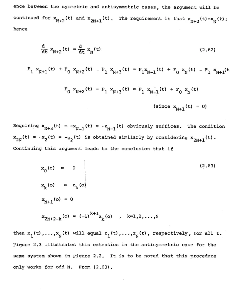
Figure 2.3 illustrates this extension in the antisymmetric case for the
same system shown in Figure 2.2. It is to be noted that this procedure
-48-substate
x7=
7
5
6
I9
z3
X,=z1
subsystem
* 7 * t - -Aqr1- 1i ii 4 i -.. -. I bindex
10
-Z 2 x 8= -z4Figure 2.3
Imbedding an antisymetric tridiagonal system with an
odd number of subsystems in a circulant system.
x
4=
4
z
4 x5=z5
x3=
3
z
3 9 x2=
z
2
0 I I I I I'N+2(0 = N+-1 )(2.64)
and so the requirement that
N+
2 (t) equals zN (t) is only met for odd N.Imbedding an antisymmetric tridiagonal system in a circulant system
when N is even will now be discussed. Suppose the system matrix of the
circulant system in which this antisymmetric system is imbedded has the
same form as the system matrix A in (2.60), only now the order of the
circulant system is as yet unspecified. It is further supposed that
sub-states
x1 (t) ,... ,xN(t) of thecirculant
system are to equalz
1 (t) ,. . .,ZN(t)? respectively, for all time. Of course, the immediate implication is that
x
(t) andN+i(t)
are both identically zero. By examining the derivativesof xN+1t) ,....,x2N (t), the following relations are obtained:
xN+
2(t) = zN (t) (2.65)x
(t)
= -zN-l(t) xN t) = N-t)'N+4
N-2
X2N (t) =z2 (t)x2l
X2N+l M
(t)
= -z (t)
-ZI1t
For odd N, the identity is x2N+l(t) =
z
(t), and so subsystems 0 and (2N+l) could be "tied together" to complete the circulant system. Inthe case of even N being considered here, tying together subsystems 0


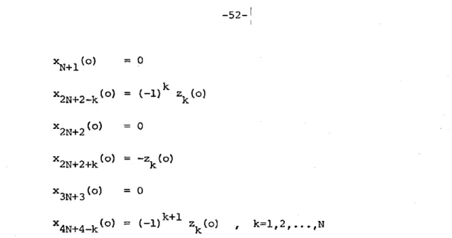

![Figure 2.5 (from [32]) . Illustration of the classical vehicle traffic loop.](https://thumb-eu.123doks.com/thumbv2/123doknet/14476504.523303/54.917.144.842.196.1032/figure-illustration-classical-vehicle-traffic-loop.webp)
![Figure 2.6 A uniform longitudinal power system consisting of N generators [49]](https://thumb-eu.123doks.com/thumbv2/123doknet/14476504.523303/60.917.111.834.77.1039/figure-uniform-longitudinal-power-consisting-n-generators.webp)