A new formulation for the ionospheric cross polar cap potential including saturation effects

(1)

HAL Id: hal-00318077

https://hal.archives-ouvertes.fr/hal-00318077

Submitted on 21 Dec 2005

HAL is a multi-disciplinary open access

archive for the deposit and dissemination of

sci-entific research documents, whether they are

pub-lished or not. The documents may come from

teaching and research institutions in France or

abroad, or from public or private research centers.

L’archive ouverte pluridisciplinaire HAL, est

destinée au dépôt et à la diffusion de documents

scientifiques de niveau recherche, publiés ou non,

émanant des établissements d’enseignement et de

recherche français ou étrangers, des laboratoires

publics ou privés.

A new formulation for the ionospheric cross polar cap

potential including saturation effects

A. J. Ridley

To cite this version:

A. J. Ridley. A new formulation for the ionospheric cross polar cap potential including saturation

ef-fects. Annales Geophysicae, European Geosciences Union, 2005, 23 (11), pp.3533-3547. �hal-00318077�

(2)

SRef-ID: 1432-0576/ag/2005-23-3533 © European Geosciences Union 2005

Annales

Geophysicae

A new formulation for the ionospheric cross polar cap potential

including saturation effects

A. J. Ridley

University of Michigan, Ann Arbor, Michigan, USA

Received: 28 February 2005 – Revised: 18 October 2005 – Accepted: 20 October 2005 – Published: 21 December 2005

Abstract. It is known that the ionospheric cross polar cap

potential (CPCP) saturates when the interplanetary magnetic field (IMF) Bz becomes very large. Few studies have

of-fered physical explanations as to why the polar cap poten-tial saturates. We present 13 events in which the recon-nection electric field (REF) goes above 12 mV/m at some time. When these events are examined as typically done in previous studies, all of them show some signs of saturation (i.e., over-prediction of the CPCP based on a linear relation-ship between the IMF and the CPCP). We show that by tak-ing into account the size of the magnetosphere and the fact that the post-shock magnetic field strength is strongly depen-dent upon the solar wind Mach number, we can better spec-ify the ionospheric CPCP. The CPCP (8) can be expressed as 8=(10−4_v2₊_11.7B(1−e−Ma/3₎_sin3_(θ/_2))r

ms/9 (where

vis the solar wind velocity, B is the combined Y and Z com-ponents of the interplanetary magnetic field, Mais the solar

wind Mach number, θ =acos(Bz/B), and rms is the

stand-off distance to the magnetopause, assuming pressure-balance between the solar wind and the magnetosphere). This is a simple modification of the original Boyle et al. (1997) for-mulation.

Keywords. Ionosphere (Electric fields and currents;

Po-lar ionosphere) – Magnetospheric physics (SoPo-lar wind-magnetosphere interactions)

1 Introduction

It has been shown in a number of studies that many iono-spheric electrodynamic properties can be described as being linearly related to the interplanetary magnetic field (IMF) and solar wind velocity. For example, Papitashvili et al. (1994) and Friis-Christensen et al. (1985) show that ground magnetic perturbations can be linearly related to the IMF

Bz and By components. These relationships can be com-Correspondence to: A. J. Ridley

([email protected])

bined with an ionospheric conductance pattern to determine a linear relationship between the IMF and the ionospheric potential pattern. Ridley et al. (2000) use the assimilative mapping of ionospheric electrodynamics (AMIE) technique (Richmond and Kamide, 1988) to calculate a large number of ionospheric electric potential maps from ground-based mag-netometers and show that the potentials are linearly related to the IMF Bz and By. Papitashvili and Rich (2002) show that

electric potentials derived from in-situ measurements of the ionospheric plasma flow also shows a linear relationship to the IMF. Most of the above analysis was completed for small magnitude IMF time periods.

Only a few studies have attempted to examine the satura-tion that may occur under strong driving of the solar wind and IMF. Reiff et al. (1981) compare in-situ measurements of ionospheric plasma flow (or electric fields and the result-ing potential) to different magnetospheric couplresult-ing functions (such as the Kan and Lee, 1979, function). They find that us-ing an amplified magnetic field (due to the bow shock com-pression) works best, but that the amplified field has to be limited to get the best fits. The best amplification factor is 7–8, with a limiting value of ∼ 60 (corresponding to a maxi-mum IMF of ∼ 8 nT).

Weimer et al. (1990) investigate the saturation of the au-roral electrojet (AE) index to both the IMF Bz and the

so-lar wind velocity (V ) multiplied by Bz. They show that the

maximum AE reaches a saturation value at Bz=−15 nT, or

V Bz=−8 mV/m. They further point out that the AE index

has been related to the cross polar cap potential (CPCP) (Ahn et al., 1984), so this indicates that the CPCP most likely sat-urates at similar values.

Russell et al. (2000) examine the high-latitude ionospheric electric potential and Joule heating saturation during the 24– 25 September 2000 storm. They attempt to show that the high-latitude features saturate while the ring current injec-tion rate does not. They further argue that the saturainjec-tion takes place when the solar wind velocity times Bz(i.e., the Y

com-ponent of the interplanetary electric field, or IEF) reaches a level of 3 mV/m. This is an equivalent magnetic field Bzof

(3)

3534 A. J. Ridley: Ionospheric potential saturation 7.5 nT with a solar wind speed of 400 km/s (similar to the

Reiff et al., 1981, value). Russell et al. (2001) show five time periods which arguably show signs of saturation in the potential and Joule heating. They continue to state that the saturation occurs near an IEF of 3 mV/m. Liemohn and Rid-ley (2002) take issue with the claims of saturation stated by Russell et al. (2001). They argue that the presented events can be fit with a linear function with similar error, and that the saturation occurs closer to 10 mV/m.

Nagatsuma (2002) shows that, on a statistical basis, the saturation occurs around 5 mV/m (or a Bzof 12.5 nT). He

in-cludes all available data from 1995–1999, which was during solar minimum and the rise to solar maximum. From Fig. 3 in their study, there is an indication that the relationship may be more complicated than simple saturation – there is a huge scatter in the points above 5 mV/m. The Nagatsuma (2002) study uses the polar cap index (PCI) as a proxy for the CPCP. Troshichev et al. (1996) show that the PCI can be related to the ionospheric potential by 8=19.35P CI +8.78, where 8 is the ionospheric CPCP in kV. Ridley and Kihn (2004) also show that the PCI is linearly related to the CPCP.

In Shepherd et al. (2002), the SuperDARN radar data in-dicate that the ionospheric potential saturates at an IEF of approximately 15–20 mV/m. This study uses 1638 10-min time periods in which there was very steady IMF and solar wind to show that the potential rarely reaches above 100 kV, which is much lower than other techniques indicate.

Siscoe et al. (2002) is one of the only studies that at-tempts to explain why the potential saturates. They argue that the saturation of the cross polar cap potential is an in-ternal process – the region 1 currents flowing into the iono-sphere tend to reduce the magnetic field near the subsolar magnetosphere, inhibiting reconnection. Equation (13) of the Siscoe et al. (2002) study relates the ionospheric cross polar cap potential 8pc (i.e. 8 above) to the electric field

(ESW) and pressure (pSW) in the solar wind, the IMF clock

angle (F (θ )), the dipole strength (D), a geometrical factor (ξ ), and the ionospheric conductance (60):

8pc=

57.6Erp1/3swD4/3F (θ )

p1/2swD +0.0125ξ 60ErF (θ )

(1) where 8pcis in kV . This formulation takes into account the

compression of the magnetosphere due to the solar wind dy-namic pressure, the reconnection efficiency, and those terms included directly above. Shepherd et al. (2003) show that in order to get the SuperDARN measurements of the satura-tion to match the Siscoe et al. (2002) formulasatura-tion, the iono-spheric conductance has to be 23 mhos, which is rather high. This could also indicate that the SuperDARN radar computed CPCP during saturated events may be too low.

The present study suggests that the saturation of the iono-spheric potential may actually be an external process. We present ionospheric cross polar cap potentials derived from the assimilative mapping of ionospheric electrodynamics (AMIE) technique (Richmond and Kamide, 1988), using the output presented in Ridley and Kihn (2004). These AMIE

runs were made with well over 100 magnetometers, and have been shown to reproduce ion flow measurements made by low altitude satellites, even during disturbed time periods (Bekerat et al. 2005; Kihn et al., 2005). There are inher-ent problems with computing the ionospheric cross polar cap potential with any technique: (1) With AMIE, using only magnetometers, one can argue that the patterns are strongly dependent upon the conductance. Indeed, this was pointed out by Ridley and Kihn (2004), who showed that there is a seasonal difference between the PCI estimated CPCP and the AMIE derived potential. It is unknown whether this is a problem with AMIE or the polar cap index. (2) Low-altitude satellites only measure a single slice of the potential pattern, so, it is thought that the measured CPCP is only a lower esti-mate, since the satellite may not pass through the maximum or minimum potential (Ober et al., 2003). In addition, since the satellites take 20 min to cross the pattern, the inferred po-tential may be a combination of different patterns. (3) Radars can not measure the entire pattern at one time, and the maxi-mum and minimaxi-mum in potential can go to lower latitudes than the radars, causing an underestimate of the potential (Shep-herd et al., 2003).

Many of the events discussed here have been shown to be saturated in other studies before this one (e.g. Nagatsuma, 2002; Shepherd et al., 2002; Hairston et al., 2003; Siscoe et al., 2004). Russell et al. (2000, 2001), and Liemohn and Ridley (2002) also present AMIE results discussing the idea of the saturation of the cross polar cap potential, showing that AMIE can be used to describe the potential during strong driving.

One of the problems with examining how the satura-tion of the cross polar cap potential occurs is that there are only a few time periods in which the IMF is extremely large compared to the number of time periods in which the IMF is small. In order to overcome this difficulty, this study only examines time periods surrounding and includ-ing events in which the reconnection electric field (REF) ex-ceeds 12 mV/m. The REF is defined as by Sonnerup (1974) and Kan and Lee (1979):

Er=V Byzsin2(θ/2), (2)

where Byz=

q B2

z+By2, and θ = cos−1(Bz/Byz), and V is the

solar wind speed.

The 12 mV/m limit allows an examination of the individ-ual events and may allow a general cause for the saturation of the potential to be illuminated. In addition, 12 mV/m is four times the value suggested by Russell et al. (2001) and Reiff et al. (1981), less than twice the value suggested by Weimer et al. (1990), and just over the value suggested by Liemohn and Ridley (2002). This value is a good compromise between using more events because of a value too low and using few events because of a very high value; both of which would tend to skew the results.

There is also a question of what time-scales to use. The AMIE runs were conducted using a 1 min time-step. It is known that there are large errors propagating solar wind data

(4)

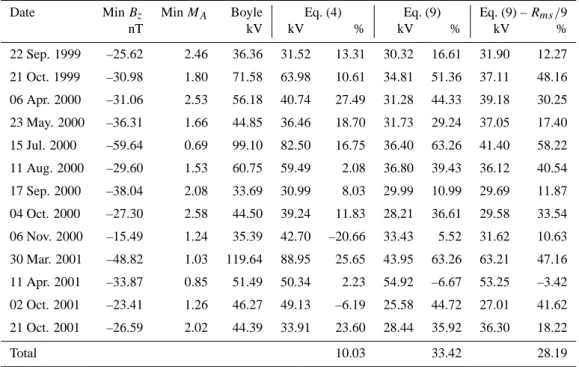
Table 1. A summary of the values associated with the 13 events. The columns are the event starting date, the minimum IMF Bzduring the

period, the minimum Alfv´en Mach number, the RMS difference between the AMIE CPCP and the Boyle et al. (1997) formulation for the 48 hour period, the RMS error using Eq. (4), the decrease in the error using this formulation over the Boyle et al. (1997) formulation, the RMS

error using Eq. (9), the decrease in the error over the Boyle et al. (1997) formulation, the RMS error using Eq. (9), but leaving out the Rms/9

term, and the decrease in the error using this formulation over the Boyle et al. (1997) formulation.

Date Min Bz Min MA Boyle Eq. (4) Eq. (9) Eq. (9) – Rms/9

nT kV kV % kV % kV % 22 Sep. 1999 –25.62 2.46 36.36 31.52 13.31 30.32 16.61 31.90 12.27 21 Oct. 1999 –30.98 1.80 71.58 63.98 10.61 34.81 51.36 37.11 48.16 06 Apr. 2000 –31.06 2.53 56.18 40.74 27.49 31.28 44.33 39.18 30.25 23 May. 2000 –36.31 1.66 44.85 36.46 18.70 31.73 29.24 37.05 17.40 15 Jul. 2000 –59.64 0.69 99.10 82.50 16.75 36.40 63.26 41.40 58.22 11 Aug. 2000 –29.60 1.53 60.75 59.49 2.08 36.80 39.43 36.12 40.54 17 Sep. 2000 –38.04 2.08 33.69 30.99 8.03 29.99 10.99 29.69 11.87 04 Oct. 2000 –27.30 2.58 44.50 39.24 11.83 28.21 36.61 29.58 33.54 06 Nov. 2000 –15.49 1.24 35.39 42.70 –20.66 33.43 5.52 31.62 10.63 30 Mar. 2001 –48.82 1.03 119.64 88.95 25.65 43.95 63.26 63.21 47.16 11 Apr. 2001 –33.87 0.85 51.49 50.34 2.23 54.92 –6.67 53.25 –3.42 02 Oct. 2001 –23.41 1.26 46.27 49.13 –6.19 25.58 44.72 27.01 41.62 21 Oct. 2001 –26.59 2.02 44.39 33.91 23.60 28.44 35.92 36.30 18.22 Total 10.03 33.42 28.19

from satellites to the magnetopause that can be on the order of 10 min or more (Ridley, 2000). It is further known that the ionospheric convection can change on time-scales of 12 min (Ridley et al., 1998). To balance the error of the propagation with the time-scales of changes in the potential, we averaged all of the data to 15 min. This is the same resolution of the Polar Cap index data used in other studies (Nagatsuma, 2002, 2004). While this will tend to wash out the extremes in the potential, the overall time evolution of the potential should be well maintained. During many of the events, the IMF and solar wind have large-scale features that last for hours, implying that the potential should vary slowly through out the time periods.

This paper first suggests that using the Boyle et al. (1997) formulation as the expected potential is not physically accu-rate, since the length of the reconnection line is not consid-ered. To account for this, the definition of the relationship between the potential and the solar wind and IMF is altered. The derived potential still over-predicts the AMIE derived potential in a few events. This implies that these events are saturated. It is then suggested that the solar wind Alfv´en Mach number may influence the potential, so the Boyle et al. (1997) formulation is further altered to include the solar wind Alfv´en Mach number. When this is done, the modeled and measured potential agree much better than without the mod-ifications. It is suggested that the mechanism for the satura-tion of the ionospheric potential may be external to the

mag-netosphere, and not an internal mechanism, as suggested by the Siscoe et al. (2002) study.

2 Results

Figures 1–4 show 13 periods in which the reconnection elec-tric field (REF) becomes larger than 12 mV/m for some in-terval of time. For each event, we show the Bzand By

com-ponents of the IMF, the cross polar cap potential from AMIE and the CPCP estimated by an analytical function that as-sumes a linear relationship between the IMF and the iono-spheric potential. This linear analytical function is by Boyle et al. (1997):

8 =10−4v2+11.7B sin3(θ /2), (3)

where we took B=Byz, θ as defined above, and v=vx. Each

cluster of plots also includes two scatter plots that demon-strate various ways in which the ionospheric cross polar cap potential can be shown to have saturation. The upper scatter plot shows the CPCP estimated by Boyle et al. (1997) and the CPCP from AMIE, both as a function of the reconnec-tion electric field, as defined by Eq. (2). The lower scatter plot shows the AMIE CPCP versus the Boyle et al. (1997) estimated CPCP, with a line showing where they would be equal. In addition, there is an indication of the root mean squared (RMS) difference between the two estimates.

(5)

3536 A. J. Ridley: Ionospheric potential saturation Figures

A. September 22-23, 1999 (Boyle Formulation)

11 21 07 17 Sep 22 to 23, 1999 UT Hours 0 100 200 300 400 Potential (kV) -30 -20 -10 0 10 20 30 Bz, By (nT) 0 5 10 15 REF (mV/m) 0 100 200 300 400 Potential (kV) 0 100 200 300 400 AMIE Potential (kV) 0 100 200 300 400 Boyle Potential (kV) Err : 36.4 kV

B. October 21-22, 1999 (Boyle Formulation)

11 21 07 17 Oct 21 to 22, 1999 UT Hours 0 100 200 300 400 Potential (kV) -40 -20 0 20 40 Bz, By (nT) 0 5 10 15 20 REF (mV/m) 0 100 200 300 400 Potential (kV) 0 100 200 300 400 AMIE Potential (kV) 0 100 200 300 400 Boyle Potential (kV) Err : 71.6 kV

C. April 4-5, 2000 (Boyle Formulation)

11 21 07 17 Apr 06 to 07, 2000 UT Hours 0 100 200 300 400 Potential (kV) -40 -20 0 20 40 Bz, By (nT) 0 5 10 15 20 REF (mV/m) 0 100 200 300 400 Potential (kV) 0 100 200 300 400 AMIE Potential (kV) 0 100 200 300 400 Boyle Potential (kV) Err : 56.2 kV

Fig. 1.The upper-left plot in each cluster shows the IMF Bz(solid) and IMF By(dashed). The lower-left plot

shows the ionospheric cross polar cap potential (CPCP) as specified by AMIE (solid) and estimated from the Boyle et al. (1997) formulation (dashed). The upper-right plot shows the Boyle et al. (1997) (stars) and AMIE CPCP (diamonds) versus the reconnection electric field. The bottom-right plot show the AMIE CPCP versus the Boyle et al. (1997) formulation potential.

26

Fig. 1. The upper-left plot in each cluster shows the IMF Bz

(solid) and IMF By(dashed). The lower-left plot shows the

iono-spheric cross polar cap potential (CPCP) as specified by AMIE (solid) and estimated from the Boyle et al. (1997) formulation (dashed). The upper-right plot shows the Boyle et al. (1997) (stars) and AMIE CPCP (diamonds) versus the reconnection electric field. The bottom-right plot show the AMIE CPCP versus the Boyle et al. (1997) formulation potential.

These clusters of plots show three different ways in which saturation of the ionospheric CPCP has typically been shown: (1) the time series plots show that the Boyle et al. (1997) estimation of the CPCP typically becomes larger than the AMIE CPCP when the IMF Bzcomponent becomes large

and negative; (2) the upper scatter plot shows that the Boyle et al. (1997) estimated CPCP is linear for large REFs, while the AMIE CPCP is significantly lower than this linear esti-mate; and (3) when the Boyle et al. (1997) estimated and the AMIE CPCPs are plotted against each other, the Boyle et al. (1997) estimated potentials are much larger than the AMIE values. While the data are shown differently, each of these three plots show exactly the same thing: a linear relationship between the reconnection electric field and the ionospheric cross polar cap potential overestimates the potential when the REF becomes large. All of the events show this to be true. The exact value of the REF at which this overestima-tion starts to occur can be debated, but it is clear that it does occur in all of the events.

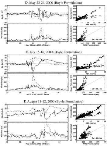
D. May 23-24, 2000 (Boyle Formulation)

01 11 21 07 17 May 23 to 24, 2000 UT Hours 0 100 200 300 400 500 Potential (kV) -40 -20 0 20 40 Bz, By (nT) 0 5 10 15 20 25 REF (mV/m) 0 100 200 300 400 500 Potential (kV) 0 100 200 300 400 500 AMIE Potential (kV) 0 100 200 300 400 500 Boyle Potential (kV) Err : 44.9 kV

E. July 15-16, 2000 (Boyle Formulation)

00 10 20 06 16 Jul 15 to 16, 2000 UT Hours 0 200 400 600 800 Potential (kV) -60 -40 -20 0 20 40 60 Bz, By (nT) 0 20 40 60 REF (mV/m) 0 200 400 600 800 Potential (kV) 0 200 400 600 800 AMIE Potential (kV) 0 200 400 600 800 Boyle Potential (kV) Err : 99.1 kV

F. August 11-12, 2000 (Boyle Formulation)

01 11 21 07 17 Aug 11 to 12, 2000 UT Hours 0 100 200 300 400 Potential (kV) -40 -20 0 20 40 Bz, By (nT) 0 5 10 15 20 REF (mV/m) 0 100 200 300 400 Potential (kV) 0 100 200 300 400 AMIE Potential (kV) 0 100 200 300 400 Boyle Potential (kV) Err : 60.8 kV

Fig. 2. Three more events in the same format as Figure 1.

27

Fig. 2. Three more events in the same format as Fig. 1.

In most previous studies of the saturation of the cross polar cap potential (e.g. Russell et al., 2001; Merkine et al., 2003; Nagatsuma, 2002), they show plots such as Figs. 1–4, imply-ing a relationship between an electric field and a potential. However there is something missing in this relationship – a length. An electric potential is the integral of an electric field along a path of some length. The above plots do not indicate any length scale at all.

This can be problematic, because when the reconnection electric field becomes large, often the solar wind density and velocity also become large. This compresses the magneto-sphere, reducing the length-scale for the integration of the electric field. That implying that the cross magnetospheric potential could possibly decrease.

By modifying the Boyle et al. (1997) formulation to in-clude a length scale, we can better relate the solar wind and IMF to the ionospheric CPCP. While the Boyle et al. (1997) formulation technically does not contain an electric field (since the first term only has a v2, and the second term does not contain a velocity), it should still be dependent upon the size of the magnetosphere. Multiplying by a ratio of the size of the magnetosphere to a nominal size, this size depen-dence is achieved:

8=(10−4v2+11.7B sin3(θ/2))rms

(6)

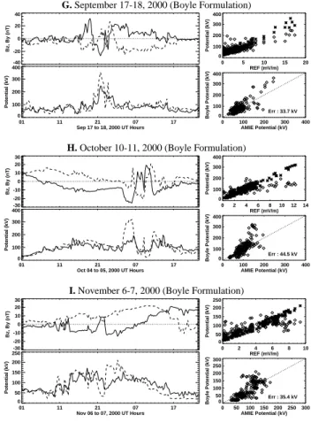
G. September 17-18, 2000 (Boyle Formulation) 01 11 21 07 17 Sep 17 to 18, 2000 UT Hours 0 100 200 300 400 Potential (kV) -40 -20 0 20 40 Bz, By (nT) 0 5 10 15 20 REF (mV/m) 0 100 200 300 400 Potential (kV) 0 100 200 300 400 AMIE Potential (kV) 0 100 200 300 400 Boyle Potential (kV) Err : 33.7 kV

H. October 10-11, 2000 (Boyle Formulation)

01 11 21 07 17 Oct 04 to 05, 2000 UT Hours 0 100 200 300 400 Potential (kV) -30 -20 -10 0 10 20 30 Bz, By (nT) 0 2 4 6 8 10 12 14 REF (mV/m) 0 100 200 300 400 Potential (kV) 0 100 200 300 400 AMIE Potential (kV) 0 100 200 300 400 Boyle Potential (kV) Err : 44.5 kV

I. November 6-7, 2000 (Boyle Formulation)

01 11 21 07 17 Nov 06 to 07, 2000 UT Hours 0 50 100 150 200 250 Potential (kV) -30 -20 -10 0 10 20 30 Bz, By (nT) 0 2 4 6 8 10 REF (mV/m) 0 50 100 150 200 250 Potential (kV) 0 50 100150 200 250300 AMIE Potential (kV) 0 50 100 150 200 250 300 Boyle Potential (kV) Err : 35.4 kV

Fig. 3. Three more events in the same format as Figure 1.

28

Fig. 3. Three more events in the same format as Fig. 1.

The radius of the magnetosphere (rms) can be approximated

through a pressure balance between the solar wind pressure and the magnetospheric magnetic field pressure (in Re):

rms=

(2Bs)2

2µ0Psw

!1/6

. (5)

Bsis the surface magnetic field, and Pswis the ram and

mag-netic pressure of the solar wind:

Psw=

B2

2µ0

+nMpv2. (6)

Where N is the solar wind number density, B is the mag-nitude of the IMF, and Mp is the mass of a proton.

Typi-cally, the solar wind ram pressure (nMpv2) is almost an

or-der of magnitude larger than the magnetic pressure. In these extreme cases, though, the magnetic pressure can become comparable to the ram pressure, so it needs to be included. It should be noted that the radius of the magnetosphere along the Earth-Sun line has a seasonal dependence and a local time dependence because of the rotational axis tilt and the offset of Earth’s dipole from the center of the planet. The effect on the radius of the magnetosphere should be less than about five percent, though. Furthermore, during periods in which the magnetic field in the solar wind becomes large, the shape of the magnetopause can be distorted (e.g. Raeder

J. March 30-31, 2001 (Boyle Formulation)

01 11 21 07 17 Mar 30 to 31, 2001 UT Hours 0 200 400 600 800 Potential (kV) -60 -40 -20 0 20 40 60 Bz, By (nT) 0 10 20 30 40 REF (mV/m) 0 200 400 600 800 Potential (kV) 0 100 200 300 400 500 600 700 AMIE Potential (kV) 0 100 200 300 400 500 600 700 Boyle Potential (kV) Err : **** kV

K. April 11-12, 2001 (Boyle Formulation)

01 11 21 07 17 Apr 11 to 12, 2001 UT Hours 0 100 200 300 400 Potential (kV) -40 -20 0 20 40 Bz, By (nT) 0 5 10 15 20 REF (mV/m) 0 100 200 300 400 Potential (kV) 0 100 200 300 400 AMIE Potential (kV) 0 100 200 300 400 Boyle Potential (kV) Err : 51.5 kV

L. October 2-3, 2001 (Boyle Formulation)

01 11 21 07 17 Oct 02 to 03, 2001 UT Hours 0 100 200 300 Potential (kV) -30 -20 -10 0 10 20 30 Bz, By (nT) 0 2 4 6 8 10 12 REF (mV/m) 0 100 200 300 Potential (kV) 0 50 100 150 200 250 300 AMIE Potential (kV) 0 50 100 150 200 250 300 Boyle Potential (kV) Err : 46.3 kV

M. October 21-22, 2000 (Boyle Formulation)

11 21 07 17 Oct 21 to 22, 2001 UT Hours 0 100 200 300 400 Potential (kV) -30 -20 -10 0 10 20 30 Bz, By (nT) 0 5 10 15 REF (mV/m) 0 100 200 300 400 Potential (kV) 0 100 200 300 400 AMIE Potential (kV) 0 100 200 300 400 Boyle Potential (kV) Err : 44.4 kV

Fig. 4. Four more events in the same format as Figure 1. 29

Fig. 4. Four more events in the same format as Fig.1.

et al., 2001; Siscoe et al., 2002, 2004). Although this dis-tortion should be taken into account, it is most likely highly dependent on the direction of the IMF (i.e., parallel versus perpendicular shocks), and therefore one would need a global magnetospheric model to do this. Because we are not using a large-scale model of the magnetosphere in this research, it is beyond the scope of the current study.

In addition, Alpha particles are not used in the calculation of the solar wind pressure. At times, the Alpha particle pop-ulation can exceed 10%. Because they are four times heavier than the protons, they can actually account for 40% of the pressure. This 40% error would cause an error in the magne-topause stand-off distance of approximately 5.5%.

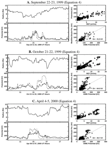
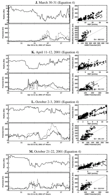
Figures 5–8 show the pressure balanced radius of the mag-netosphere, the AMIE CPCP and the estimated potential us-ing Eq. (4). In addition, the RMS differences between the AMIE potentials and Eq. (4) estimated potentials are dis-played on the plots. Table 1 summarizes all of the errors

(7)

3538 A. J. Ridley: Ionospheric potential saturation A. September 22-23, 1999 (Equation 4) 11 21 07 17 Sep 22 to 23, 1999 UT Hours 0 100 200 300 400 Potential (kV) 4 6 8 10 12 Radius (Re) 0 5 10 15 REF (mV/m) 0 100 200 300 400 Potential (kV) 0 100 200 300 400 AMIE Potential (kV) 0 100 200 300 400

Modified Boyle Pot. (kV)

Err : 31.5 kV B. October 21-22, 1999 (Equation 4) 11 21 07 17 Oct 21 to 22, 1999 UT Hours 0 100 200 300 400 Potential (kV) 5 6 7 8 9 10 Radius (Re) 0 5 10 15 20 REF (mV/m) 0 100 200 300 400 Potential (kV) 0 100 200 300 400 AMIE Potential (kV) 0 100 200 300 400

Err : 64.0 kV C. April 4-5, 2000 (Equation 4) 11 21 07 17 Apr 06 to 07, 2000 UT Hours 0 100 200 300 400 Potential (kV) 4 6 8 10 12 Radius (Re) 0 5 10 15 20 REF (mV/m) 0 100 200 300 400 Potential (kV) 0 100 200 300 400 AMIE Potential (kV) 0 100 200 300 400

Err : 40.7 kV

Fig. 5. The same three events in Figure 1, plotted in the same way, except Equation 4 was used rather

than estimating the CPCP with Boyle et al. (1997). The top plot is the radius of the magnetosphere, as estimated by Equation 5.

30

Fig. 5. The same three events in Fig. 1, plotted in the same way,

except Eq. (4) was used rather than estimating the CPCP with Boyle et al. (1997). The top plot is the radius of the magnetosphere, as estimated by Eq. (5).

associated with all of the events. The percentage differences that are shown in the table are changes in the performance compared to the Boyle et al. (1997) formulation. The RMS difference between the potentials decreases by 10% over the Boyle et al. (1997) formulation when the magnetospheric size is considered.

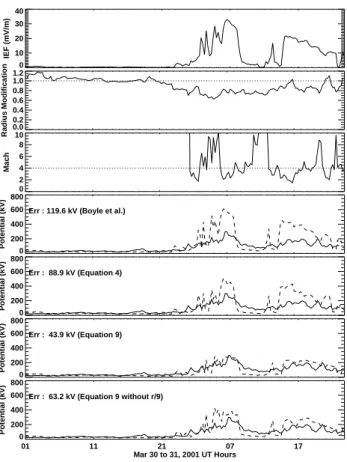
Figures 5–8 compared to Figs.1–4 show a decrease in the amount of over-prediction of the ionospheric potential in most of the events. Some of these events show very little saturation at all (22 September 1999; 17 September 2000; 11 April 2001; 21 October 2001), implying that considering the radius of the magnetosphere may be important when exam-ining large IMF and solar wind events. Some events (namely 21 October 1999; 15 July 2000; 30 March 2001; and 2 Octo-ber 2001) still show significant over-predictions of the CPCP. It is evident that a modified formulation must be determined that further takes into account the saturation of the potential. Let us consider a single event chosen at random, 30–31 March 2001. Figure 9 shows all of the relevant quantities for this time period, such as the reconnection electric field and the radius modification factor (rms/9, as discussed above).

The third plot shows the solar wind Alfv´en Mach number,

D. May 23-24, 2000 (Equation 4) 01 11 21 07 17 May 23 to 24, 2000 UT Hours 0 100 200 300 400 500 Potential (kV) 4 6 8 10 12 Radius (Re) 0 5 10 15 20 25 REF (mV/m) 0 100 200 300 400 500 Potential (kV) 0 100 200 300 400 500 AMIE Potential (kV) 0 100 200 300 400 500

Err : 36.5 kV E. July 15-16, 2000 (Equation 4) 00 10 20 06 16 Jul 15 to 16, 2000 UT Hours 0 200 400 600 800 Potential (kV) 4 6 8 10 12 14 Radius (Re) 0 20 40 60 REF (mV/m) 0 200 400 600 800 Potential (kV) 0 100 200 300 400 500 600 700 AMIE Potential (kV) 0 100 200 300 400 500 600 700

Err : 82.5 kV F. August 11-12, 2000 (Equation 4) 01 11 21 07 17 Aug 11 to 12, 2000 UT Hours 0 100 200 300 400 Potential (kV) 4 6 8 10 12 14 Radius (Re) 0 5 10 15 20 REF (mV/m) 0 100 200 300 400 Potential (kV) 0 100 200 300 400 AMIE Potential (kV) 0 100 200 300 400

Err : 59.5 kV

Fig. 6. The same three events in Figure 2, plotted in the same way as Figure 5.

31

Fig. 6. The same three events in Fig. 2, plotted in the same way as

Fig. 5.

which is defined as:

Ma= Vsw Ca , (7) where Ca= B pµ0nMp . (8)

The fourth plot shows the AMIE CPCP as well as the CPCP estimated from Boyle et al. (1997), while the fifth plot shows the AMIE and Eq. (4) estimated CPCPs. It is interest-ing to note that when the potential is saturated (i.e., the pre-dicted potential is significantly larger than the AMIE value), the Alfv´en Mach number is less than four. Indeed, this is true of all other events, and could in fact be the cause of the saturation.

Taking the Alfv´en Mach number into consideration, we can express the ionospheric cross polar cap potential as:

8=(10−4v2+11.7B(1 − e−Ma/3₎_sin3_(θ/₂₎₎rms

9 . (9)

The term (1−e−Ma/3₎_{, which multiplies the magnetic} field, will be justified below, when the physics of the bow shock is discussed. When the Alfv´en Mach number is in its typical range (approximately eight), the last term is 0.93,

(8)

G. September 17-18, 2000 (Equation 4) 01 11 21 07 17 Sep 17 to 18, 2000 UT Hours 0 100 200 300 400 Potential (kV) 4 6 8 10 12 14 Radius (Re) 0 5 10 15 20 REF (mV/m) 0 100 200 300 400 Potential (kV) 0 100 200 300 400 AMIE Potential (kV) 0 100 200 300 400

Err : 31.0 kV H. October 10-11, 2000 (Equation 4) 01 11 21 07 17 Oct 04 to 05, 2000 UT Hours 0 100 200 300 400 Potential (kV) 5 6 7 8 9 10 11 Radius (Re) 0 2 4 6 8 10 12 14 REF (mV/m) 0 100 200 300 400 Potential (kV) 0 100 200 300 400 AMIE Potential (kV) 0 100 200 300 400

Err : 39.2 kV I. November 6-7, 2000 (Equation 4) 01 11 21 07 17 Nov 06 to 07, 2000 UT Hours 0 50 100 150 200 250 Potential (kV) 4 6 8 10 12 Radius (Re) 0 2 4 6 8 10 REF (mV/m) 0 50 100 150 200 250 Potential (kV) 0 50 100 150 200 250300 AMIE Potential (kV) 0 50 100 150 200 250 300

Err : 42.7 kV

32

Figure 5.

so it does not modify the potential very much at all. As the Mach number decreases significantly (i.e. the magnetic field becomes very large, or the solar wind density decreases dramatically – both of which occur in magnetic clouds) the last term decreases. At a Mach number of three, the term is 0.63, and at a Mach number of one, it is 0.28. The ef-fect of this term on the 30–31 March 2001 event is shown in the sixth plot in Fig. 9. For comparison, the bottom plot in Fig. 9, shows the event using Eq. (9), but without the magne-tospheric size correction factor (rms/9). The smallest error

between the AMIE CPCP and the other formulations occurs when Eq. (9) is used.

Figure 10 shows examples of how this term modifies the ionospheric potential as a function of the reconnection electric field, solar wind velocity and solar wind density. The plots on the left have an input solar wind velocity of 400 km/s, while those on the right have an input velocity of 800 km/s. From top to bottom, the input solar wind densities are 1, 5, and 20 cm−3_{. These plots show that as the solar}

wind number density and velocity increase, the saturation of the potential occurs at a much higher REF.

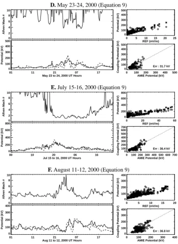
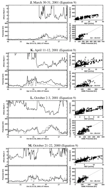
When Eq. (9) is applied to all of the events, Figs. 11–14 result. These plots show the Alfv´en Mach number and the es-timated potential using Eq. (9). The saturation is reproduced in almost all cases, and strongly suggests that the saturation

J. March 30-31 (Equation 4) 01 11 21 07 17 Mar 30 to 31, 2001 UT Hours 0 200 400 600 800 Potential (kV) 5 6 7 8 9 10 11 Radius (Re) 0 10 20 30 40 REF (mV/m) 0 200 400 600 800 Potential (kV) 0 100 200 300 400 500 600 700 AMIE Potential (kV) 0 100 200 300 400 500 600 700

Err : 88.9 kV K. April 11-12, 2001 (Equation 4) 01 11 21 07 17 Apr 11 to 12, 2001 UT Hours 0 100 200 300 400 Potential (kV) 4 6 8 10 12 14 Radius (Re) 0 5 10 15 20 REF (mV/m) 0 100 200 300 400 Potential (kV) 0 100 200 300 400 AMIE Potential (kV) 0 100 200 300 400

Err : 50.3 kV L. October 2-3, 2001 (Equation 4) 01 11 21 07 17 Oct 02 to 03, 2001 UT Hours 0 100 200 300 Potential (kV) 4 6 8 10 12 Radius (Re) 0 2 4 6 8 10 12 REF (mV/m) 0 100 200 300 Potential (kV) 0 50 100150 200 250 300 AMIE Potential (kV) 0 50 100 150 200 250 300

Err : 49.1 kV M. October 21-22, 2001 (Equation 4) 11 21 07 17 Oct 21 to 22, 2001 UT Hours 0 100 200 300 400 Potential (kV) 4 6 8 10 12 Radius (Re) 0 5 10 15 REF (mV/m) 0 100 200 300 400 Potential (kV) 0 100 200 300 400 AMIE Potential (kV) 0 100 200 300 400

Err : 33.9 kV

Fig. 8. The same four events in Figure 4, plotted in the same way as Figure 5. 33

Fig. 8. The same four events in Fig. 4, plotted in the same way as

Fig. 5.

may be tied to the Alfv´en Mach number. The RMS differ-ence is decreased by 33.4% over using simply the Boyle et al. (1997) formulation (see Table 1). Eq. (9) is a much better es-timation of the cross polar cap potential than the Boyle et al. (1997) formulation during strong driving conditions.

3 Discussion

The study by Reiff et al. (1981) discusses the fact that when the IMF is advected through the bow shock, it increases in strength. For a typical solar wind density and flow speed, the IMF can increase by a factor of four from the solar wind to the magnetosheath. In addition, as the magnetic field in the solar wind becomes larger, the ratio between the shocked magnetic field and upstream field decreases. This is because the Alfv´en Mach number decreases with increasing magnetic

(9)

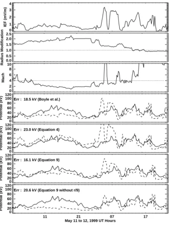
3540 A. J. Ridley: Ionospheric potential saturation 0 10 20 30 40 IEF (mV/m) 0 2 4 6 8 10 Mach 0.0 0.2 0.4 0.6 0.8 1.0 1.2 Radius Modification 0 200 400 600 800 Potential (kV)

Err : 119.6 kV (Boyle et al.)

0 200 400 600 800 Potential (kV) Err : 88.9 kV (Equation 4) 0 200 400 600 800 Potential (kV) Err : 43.9 kV (Equation 9) 01 11 21 07 17 Mar 30 to 31, 2001 UT Hours 0 200 400 600 800 Potential (kV)

Err : 63.2 kV (Equation 9 without r/9)

Fig. 9. From top to bottom: the reconnection electric field, using Equation 2; the magnetospheric

radius divided by 9; the solar wind Alfv´en Mach number; the AMIE cross polar cap potential (CPCP, solid) and the estimated CPCP using Equation 4; and the AMIE CPCP (solid) and the estimated CPCP using Equation 9. The time period is March 30-31, 2001.

34

Fig. 9. From top to bottom: the reconnection electric field, using

Eq. (2); the magnetospheric radius divided by 9; the solar wind Alfv´en Mach number; the AMIE cross polar cap potential (CPCP, solid) and the estimated CPCP using Eq. (4); and the AMIE CPCP (solid) and the estimated CPCP using Eq. (9). The time period is 30–31 March 2001.

field. Reiff et al. (1981) show that they can increase the cor-relation between the IMF and the cross polar cap potential by “shocking” the IMF up to a certain level and having values above that be constant.

Recently, Lopez et al. (2004) discuss the role of the solar wind number density in controlling the strength of the cross polar cap potential and ionospheric Joule heating. They show that the solar wind density and the magnetic field strength control the compression ratio of the bow shock. During nom-inal solar wind and IMF conditions, the magnetic field is al-ways increased by a constant factor (independent of the so-lar wind density) as it goes through the shock. As the mag-netic field increases, the solar wind density gains more con-trol over the shock compression.

This can be quantified if one only considers magnetic fields that are tangential to the bow shock (i.e., only By and

Bzcomponents of the IMF). The following set of equations

can be used to determine the increase in field strength and density across the bow shock (Roberge and Draine, 1993):

pu=nukTu (10) Csu = r γpu ρu (11) 0 5 10 15 20 0 100 200 300 400 500 Potential (kV) V=400 km/s, n=1cm-3 0 5 10 15 20 0 100 200 300 400 500 Potential (kV) V=400 km/s, n=5cm-3 0 5 10 15 20 IEF (mV/m) 0 100 200 300 400 500 Potential (kV) V=400 km/s, n=20cm-3 0 10 20 30 40 0 100 200 300 400 500 Potential (kV) V=800 km/s, n=1cm-3 0 10 20 30 40 0 100 200 300 400 500 Potential (kV) V=800 km/s, n=5cm-3 0 10 20 30 40 IEF (mV/m) 0 100 200 300 400 500 Potential (kV) V=800 km/s, n=20cm-3

Fig. 10. Examples of CPCP curves as a function of REF using Equation 9 (solid) and Equation 4 (dashed). The left curves use an input solar wind velocity of 400 km/s, while the right curves use 800 km/s. From top to bottom, the input solar wind density is changed from 1cm−3

to 5cm−3 to 20cm−3_{. The vertical line indicates when the solar wind Mach number is four. Points to the right} are less than four. It should be noted that the vertical scales are the same on all plots, but the left plots stop at REF= 20mV /m, while the right plots stop at REF= 40mV /m. The REF is altered by

changing the magnitude of the IMFBzcomponent - there is noBycomponent.

35

Fig. 10. Examples of CPCP curves as a function of REF using

Eq. (9) (solid) and Eq. (4) (dashed). The left curves use an input so-lar wind velocity of 400 km/s, while the right curves use 800 km/s. From top to bottom, the input solar wind density is changed from

1 cm−3to 5 cm−3to 20 cm−3. The vertical line indicates when the

solar wind Mach number is four. Points to the right are less than four. It should be noted that the vertical scales are the same on all plots, but the left plots stop at REF=20 mV/m, while the right plots stop at REF=40 mV/m. The REF is altered by changing the

magni-tude of the IMF Bzcomponent – there is no Bycomponent.

CAu= Bu √ µ0ρu (12) Msu= Vu Csu (13) MAu= Vu CAu (14) C = γ −1 + 2M_su−2+γ M_Au−2 (15) ρd ρu = Bd Bu = 2(γ + 1) C + q C2₊_{4(γ + 1)(2 − γ )M}−2 Au , (16)

where symbols with a subscript “u” are upstream of the bow shock, and values with a subscript “d” are downstream of the bow shock. T is the temperature of the solar wind, k is Boltzmann’s constant, γ is 5/3, nuis the solar wind number

density, ρu is the solar wind mass density, pu is the kinetic

pressure of the solar wind, Csuis the solar wind sound speed,

CAu is the solar wind Alfv´en speed, Vu is the solar wind

speed, and MAu and Msu are the Alfv´en and sonic Mach

numbers, respectively.

An important consideration in this formulation is that it is for a shock in which B is perpendicular to the shock normal. This is only true (at the subsolar point) when Bx=0. When

Bxis non-zero, this formulation will be incorrect for the

sub-solar point. The relative strength of Bx to

q B2

y+Bz2 will

determine how relevant it is. During large events in which the main components of the IMF are in Bzand By, this

(10)

A. September 22-23, 1999 (Equation 9) 11 21 07 17 Sep 22 to 23, 1999 UT Hours 0 100 200 300 400 Potential (kV) 0 2 4 6 8 10 Alfven Mach # 0 5 10 15 REF (mV/m) 0 100 200 300 400 Potential (kV) 0 100 200 300 400 AMIE Potential (kV) 0 100 200 300 400 Coupling Potential (kV) Err : 30.3 kV B. October 21-22, 1999 (Equation 9) 11 21 07 17 Oct 21 to 22, 1999 UT Hours 0 100 200 300 400 Potential (kV) 0 2 4 6 8 10 Alfven Mach # 0 5 10 15 20 REF (mV/m) 0 100 200 300 400 Potential (kV) 0 100 200 300 400 AMIE Potential (kV) 0 100 200 300 400 Coupling Potential (kV) Err : 34.8 kV C. April 4-5, 2000 (Equation 9) 11 21 07 17 Apr 06 to 07, 2000 UT Hours 0 100 200 300 400 Potential (kV) 0 2 4 6 8 10 Alfven Mach # 0 5 10 15 20 REF (mV/m) 0 100 200 300 400 Potential (kV) 0 100 200 300 400 AMIE Potential (kV) 0 100 200 300 400 Coupling Potential (kV) Err : 31.3 kV

Fig. 11. The same three events in Figure 1, plotted in the same way, except Equation 9 was used

rather than estimating the CPCP with Boyle et al. (1997). The top plot is the Alfv´en Mach number.

36

Fig. 11. The same three events in Fig. 1, plotted in the same way,

except Eq. (9) was used rather than estimating the CPCP with Boyle et al. (1997). The top plot is the Alfv´en Mach number.

Typically, the sound speed in the solar wind is on the order of 50 km/s, depending on the solar wind temperature. This means that the sound Mach number is on the order of 7 to 20 (given solar wind speeds of 350 km/s–1000 km/s). The Alfv´en Mach number is typically in the range of eight for nominal solar wind and IMF conditions. These large values of MAuand Msuimply that:

Bd'

γ +1

γ −1Bu= 5/3 + 1

5/3 − 1Bu=4Bu. (17)

The magnetosheath magnetic field is approximately four times the IMF for tangential fields and nominal solar wind conditions.

Figure 15 shows the relationship between the IMF and the solar wind Alfv´en Mach number for a number of differ-ent solar wind number densities. The grey shaded region is considered nominal values (i.e., 2.5 cm−3< nu <10 cm−3

and 1 nT < Bu <10 nT). In this regime, the Alfv´en Mach

number is always above three. It is clear that, as the num-ber density of the solar wind decreases, the Mach numnum-ber also decreases, meaning that the solar wind can become sub-Alfv´enic at lower magnetic field values. For example, with a number density of 1 cm−3, an 18 nT magnetic field means a sub-Alfv´enic solar wind (if the solar wind speed is 400 km/s).

D. May 23-24, 2000 (Equation 9) 01 11 21 07 17 May 23 to 24, 2000 UT Hours 0 100 200 300 400 500 Potential (kV) 0 2 4 6 8 10 Alfven Mach # 0 5 10 15 20 25 REF (mV/m) 0 100 200 300 400 500 Potential (kV) 0 100 200 300 400 500 AMIE Potential (kV) 0 100 200 300 400 500 Coupling Potential (kV) Err : 31.7 kV E. July 15-16, 2000 (Equation 9) 00 10 20 06 16 Jul 15 to 16, 2000 UT Hours 0 200 400 600 800 Potential (kV) 0 2 4 6 8 10 Alfven Mach # 0 20 40 60 REF (mV/m) 0 200 400 600 800 Potential (kV) 0 100 200 300 400 500 600 700 AMIE Potential (kV) 0 100 200 300 400 500 600 700 Coupling Potential (kV) Err : 36.4 kV F. August 11-12, 2000 (Equation 9) 01 11 21 07 17 Aug 11 to 12, 2000 UT Hours 0 100 200 300 400 Potential (kV) 0 2 4 6 8 10 Alfven Mach # 0 5 10 15 20 REF (mV/m) 0 100 200 300 400 Potential (kV) 0 100 200 300 400 AMIE Potential (kV) 0 100 200 300 400 Coupling Potential (kV) Err : 36.8 kV

37

Fig. 11.

When the solar wind number density is 25 cm−3, the solar wind becomes sub-Alfv´enic only when the IMF is larger than 90 nT, which is a very rare occurrence. When one considers that the cores of magnetic clouds are regions of high mag-netic field strength, low temperature, and low density, they are in the exact region that can easily become sub-Alfv´enic. These are also the times in which saturation of the CPCP oc-curs.

Figure 16 offers a possible explanation for the saturation of the cross polar cap potential. This plot shows the shocked (i.e., magnetosheath) magnetic field strength as a function of the upstream magnetic field strength for a number of different solar wind number densities. If one of the lines is followed, there is a sharp, linear rise of the magnetic field when the Alfv´en Mach number is very large (i.e., Bu is small). This

line is simply Bd=4Bu. As the Mach number decreases

be-low three, the sheath field saturates at around Bd=2Bu, and

actually starts to decrease. When the Mach number passes below one, there is no longer a shock, so Eq. (16) is no longer valid.

Equation (9) multiplies the magnetic field of the Boyle et al. (1997) formulation by a factor of (1−e−Ma/3₎_{, which} has a very similar dependence on the Alfv´en Mach number as Eq. (16). Figure 17 shows the ratio of the downstream and upstream magnetic fields Eq. (16) as a function of upstream

(11)

3542 A. J. Ridley: Ionospheric potential saturation G. September 17-18, 2000 (Equation 9) 01 11 21 07 17 Sep 17 to 18, 2000 UT Hours 0 100 200 300 400 Potential (kV) 0 2 4 6 8 10 Alfven Mach # 0 5 10 15 20 REF (mV/m) 0 100 200 300 400 Potential (kV) 0 100 200 300 400 AMIE Potential (kV) 0 100 200 300 400 Coupling Potential (kV) Err : 30.0 kV H. October 10-11, 2000 (Equation 9) 01 11 21 07 17 Oct 04 to 05, 2000 UT Hours 0 100 200 300 400 Potential (kV) 0 2 4 6 8 10 Alfven Mach # 0 2 4 6 8 10 12 14 REF (mV/m) 0 100 200 300 400 Potential (kV) 0 100 200 300 400 AMIE Potential (kV) 0 100 200 300 400 Coupling Potential (kV) Err : 28.2 kV I. November 6-7, 2000 (Equation 9) 01 11 21 07 17 Nov 06 to 07, 2000 UT Hours 0 50 100 150 200 250 Potential (kV) 0 2 4 6 8 10 Alfven Mach # 0 2 4 6 8 10 REF (mV/m) 0 50 100 150 200 250 Potential (kV) 0 50 100 150 200 250 300 AMIE Potential (kV) 0 50 100 150 200 250 300 Coupling Potential (kV) Err : 33.4 kV

38

Fig. 11.

magnetic field. In addition, 4(1−e−Ma/3₎_{is over-plotted to} show that the lines almost overlay each other. This means that by taking into account the shocking of the solar wind, either with Eq. (16) (divided by four), or with a simple ex-ponential dependence, the saturation of the cross polar cap potential can be accurately modeled.

It should be noted that the solar wind velocity decreases in speed by the same ratio as the magnetic field through the shock, meaning that the electric field remains the same through the shock. At the subsolar point though, the veloc-ity decreases to zero as it approaches the magnetopause (in-dependent of the shock strength), while the magnetic field increases to some value that is most likely controlled by the shocked magnetic field strength. The original Boyle et al. (1997) formulation does not contain the velocity in the pri-mary coupling term, so the decrease in the velocity through the shock need not be compensated for in this term. The vis-cous interaction term, on the other hand, does have a v2term. It is not reduced in the formulation above because the viscous interaction takes place on the sides of the magnetosphere, af-ter the solar wind has accelerated back up to some significant fraction of the original velocity.

Recently it has been shown that during time periods of low Alfven Mach numbers, the magnetosphere can exhibit global sawtooth oscillations (J. Borovsky, personal

commu-J. March 30-31, 2001 (Equation 9) 01 11 21 07 17 Mar 30 to 31, 2001 UT Hours 0 200 400 600 800 Potential (kV) 0 2 4 6 8 10 Alfven Mach # 0 10 20 30 40 REF (mV/m) 0 200 400 600 800 Potential (kV) 0 100 200 300 400 500 600 700 AMIE Potential (kV) 0 100 200 300 400 500 600 700 Coupling Potential (kV) Err : 43.9 kV K. April 11-12, 2001 (Equation 9) 01 11 21 07 17 Apr 11 to 12, 2001 UT Hours 0 100 200 300 400 Potential (kV) 0 2 4 6 8 10 Alfven Mach # 0 5 10 15 20 REF (mV/m) 0 100 200 300 400 Potential (kV) 0 100 200 300 400 AMIE Potential (kV) 0 100 200 300 400 Coupling Potential (kV) Err : 54.9 kV L. October 2-3, 2001 (Equation 9) 01 11 21 07 17 Oct 02 to 03, 2001 UT Hours 0 100 200 300 Potential (kV) 0 2 4 6 8 10 Alfven Mach # 0 2 4 6 8 10 12 REF (mV/m) 0 100 200 300 Potential (kV) 0 50 100150 200 250 300 AMIE Potential (kV) 0 50 100 150 200 250 300 Coupling Potential (kV) Err : 25.6 kV M. October 21-22, 2000 (Equation 9) 11 21 07 17 Oct 21 to 22, 2001 UT Hours 0 100 200 300 400 Potential (kV) 0 2 4 6 8 10 Alfven Mach # 0 5 10 15 REF (mV/m) 0 100 200 300 400 Potential (kV) 0 100 200 300 400 AMIE Potential (kV) 0 100 200 300 400 Coupling Potential (kV) Err : 28.4 kV

Fig. 14. The same four events in Figure 4, plotted in the same way as Figure 11. 39

Fig. 14. The same four events in Fig. 4, plotted in the same way as

Fig. 11.

nication). It could be possible that these two phenomena both occur during similar driving conditions, and may both be ramifications of the different coupling that may occur be-tween the IMF and the magnetosphere during low Alfv´en Mach number conditions.

Obviously, this idea fits quite well with the idea proposed by Reiff et al. (1981), but it is different than other ideas of what causes the saturation of the ionospheric CPCP. One of the most popular ideas on why the CPCP saturates was put forth by Siscoe et al. (2002).

3.1 Siscoe-Hill Formulation

In a study conducted by Hill et al. (1976), it was theorized that the observation of high energy particles in the magneto-sphere of Mercury, and the lack of high energy particles in

(12)

0 20 40 60 80 100 BSW (nT) 1 10 100 Solar Wind M A N = 1 cm -3 N = 2.5N = 5 cm -3 N = 10 cm -3 N = 25 cm -3

Fig. 15. The solar wind Alfv´en Mach number as a function of the IMF strength for a number of solar

wind number densities. The solar wind speed is 400 km/s in this plot. The shaded region represents

typical values of the solar wind number density and IMF strength.

0 20 40 60 80 100 BSW (nT) 0 20 40 60 80 100 BShocked (nT) N = 1 cm-3 N = 2.5 N = 5 cm-3 N = 10 cm-3 N = 25 cm-3

Fig. 16. The magnetosheath magnetic field strength as a function of the upstream IMF strength for

a number of solar wind number densities. The bottom right area represents a region in which the

Alfv´en Mach number is less than one, so it is not considered. The shaded region represents typical

values of the solar wind number density and IMF strength. The solar wind speed is 400 km/s in this

plot.

40

Fig. 15. The solar wind Alfv´en Mach number as a function of the

IMF strength for a number of solar wind number densities. The so-lar wind speed is 400 km/s in this plot. The shaded region represents typical values of the solar wind number density and IMF strength.

0 20 40 60 80 100 BSW (nT) 1 10 100 Solar Wind M A N = 1 cm -3 N = 2.5N = 5 cm -3 N = 10 cm -3 N = 25 cm -3

Fig. 15. The solar wind Alfv´en Mach number as a function of the IMF strength for a number of solar

wind number densities. The solar wind speed is 400 km/s in this plot. The shaded region represents typical values of the solar wind number density and IMF strength.

0 20 40 60 80 100 BSW (nT) 0 20 40 60 80 100 BShocked (nT) N = 1 cm-3 N = 2.5 N = 5 cm-3 N = 10 cm-3 N = 25 cm-3

Fig. 16. The magnetosheath magnetic field strength as a function of the upstream IMF strength for

a number of solar wind number densities. The bottom right area represents a region in which the Alfv´en Mach number is less than one, so it is not considered. The shaded region represents typical values of the solar wind number density and IMF strength. The solar wind speed is 400 km/s in this plot.

40

Fig. 16. The magnetosheath magnetic field strength as a function

of the upstream IMF strength for a number of solar wind number densities. The bottom right area represents a region in which the Alfv´en Mach number is less than one, so it is not considered. The shaded region represents typical values of the solar wind number density and IMF strength. The solar wind speed is 400 km/s in this plot.

the magnetosphere of Mars could be explained by consider-ing the ionospheric conductance. They analytically showed that if the conductance is large (as in the Martian system), the high latitude cross polar cap potential can be severely limited. If the conductance is negligible, the potential may be unbounded. Hill et al. (1976) described the polar cap po-tential:

8= 8ms8iono 8ms+8iono

, (18)

where 8iono represents a maximum potential that the

ionosphere can sustain, 8ms is the magnetospheric

merging potential similar to that described above, and 8 is

0 20 40 60 80 100 BSW (nT) 1 2 3 4 Bd /B u N = 1 cm -3 N = 2.5 N = 5 cm -3 N = 10 cm -3 N = 25 cm -3

Fig. 17. The ratio of the downstream and upstream magnetic fields as a function of upstream

mag-netic field strength (i.e., Equation 16) are plotted as solid lines for five densities. The formula

4(1 − e

−Ma/3

) is over-plotted as dotted lines for the five different densities.

41

Fig. 17. The ratio of the downstream and upstream magnetic fields

as a function of upstream magnetic field strength (i.e., Eq. (16)) are

plotted as solid lines for five densities. The formula 4(1−e−Ma/3₎

is over-plotted as dotted lines for the five different densities.

the ionospheric cross polar cap potential. The Hill et al. (1976) formulation shows that the true ionospheric poten-tial is a combination of the magnetospheric merging potenpoten-tial and the amount of potential that the ionosphere can sustain. Hill et al. (1976) show that for Mercury, which has no iono-sphere, 8ionois very large, but 8msis small, so 8=8ms. On

Mars, the situation is reversed – the ionospheric potential is small, while the magnetospheric merging potential is (rela-tively) large, so 8=8iono. On Earth, it is argued, these

po-tentials are similar to each other during nominal conditions. Reiff et al. (1981) showed that the cross polar cap po-tential of Earth could be predicted quite accurately using a modification of the Hill et al. (1976) formulation. Siscoe et al. (2002) also modified this formulation and showed that it could be used to determine how the ionospheric cross po-lar cap potential will saturate for strong interplanetary elec-tric fields (i.e. 8msbecoming much larger than 8iono, so 8

pushes towards 8iono). They explain that the saturation

oc-curs when the region 1 current system causes a significant perturbation (i.e. 50% of the dipole field) at the subsolar magnetopause.

Equation (13) of the Siscoe et al. (2002) study (Eq. (1), above) relates the ionospheric cross polar cap potential to the electric field and pressure in the solar wind, the IMF clock angle, the dipole strength, and the ionospheric conductance. There are aspects of the Siscoe et al. (2002) formulation that are similar to ideas put forth here. Namely that the CPCP is an integral of the electric field over some length that is determined by the pressure in the solar wind. In addition, there is a geometrical term that describes the efficiency of the reconnection F (θ ) that is similar to one used in the Boyle et al. (1997) formulation.

This study argues that the saturation of the cross polar cap potential can be explained by phenomena external to the magnetosphere. It is argued that the internal properties of the solar wind and its interaction with a magnetized (or