Optimizing thermo-mechanical processing and material coupling parameters in numerical modeling for additive manufacturing

(1)

HAL Id: insu-02954002

https://hal-insu.archives-ouvertes.fr/insu-02954002v2

Submitted on 4 Feb 2021

HAL is a multi-disciplinary open access archive for the deposit and dissemination of sci-entific research documents, whether they are pub-lished or not. The documents may come from teaching and research institutions in France or abroad, or from public or private research centers.

L’archive ouverte pluridisciplinaire HAL, est destinée au dépôt et à la diffusion de documents scientifiques de niveau recherche, publiés ou non, émanant des établissements d’enseignement et de recherche français ou étrangers, des laboratoires publics ou privés.

Distributed under a Creative Commons Attribution| 4.0 International License

Optimizing thermo-mechanical processing and material

coupling parameters in numerical modeling for additive

manufacturing

Lamanna Antoine, Erwan Beauchesne, Pierre-Richard Dahoo, Constantin

Meis

To cite this version:

Lamanna Antoine, Erwan Beauchesne, Pierre-Richard Dahoo, Constantin Meis. Optimizing thermo-mechanical processing and material coupling parameters in numerical modeling for additive manufac-turing. Journal of Physics: Conference Series, IOP Publishing, 2021, 1730, pp.012128. �10.1088/1742-6596/1730/1/012128�. �insu-02954002v2�

(2)

Journal of Physics: Conference Series

PAPER • OPEN ACCESS

Optimizing thermo-mechanical processing and material coupling

parameters in numerical modeling for additive manufacturing

To cite this article: Lamanna Antoine et al 2021 J. Phys.: Conf. Ser. 1730 012128

(3)

Content from this work may be used under the terms of theCreative Commons Attribution 3.0 licence. Any further distribution of this work must maintain attribution to the author(s) and the title of the work, journal citation and DOI.

Published under licence by IOP Publishing Ltd

IC-MSQUARE 2020

Journal of Physics: Conference Series 1730 (2021) 012128

IOP Publishing doi:10.1088/1742-6596/1730/1/012128

1

Optimizing thermo-mechanical processing and material

coupling parameters in numerical modeling for additive

manufacturing

Lamanna Antoine1_{, Erwan Beauchesne}2_{, Dahoo Pierre-Richard}1_{and Constantin}

Meis3

1 LATMOS/IPSL, UVSQ Université Paris-Saclay, Sorbonne Université, CNRS, 78280, Guyancourt, France

2 Altair Engineering, 5-10 Rue de la Renaissance, 92160 Antony, France

3 National Institute for Nuclear Science and Technology, CEA Saclay, 91191 Gif-sur Yvette, France

E-mail: lamanna.antoine@latmos.ipsl.fr, erwan.beauchesne@altair.com, pierre.dahoo@uvsq.fr, constantin.meis@cea.fr

Abstract. Additive manufacturing (AM) is gaining increasing industrial interest. Initially

conceived to facilitate the pre-production, to manufacture efficiently and cheaply unique parts such as prototypes, it is now able to deliver parts that meet industrial production needs. In addition, AM is an effective way to achieve parts designed using topological optimization. Laser beam melting is an AM technique able to produce specific parts with mechanical properties matching industrial expectations. However, efficient production remains complex because of distortion, cracking and other failures linked to the process and to the machine parameters. The prime material being generally expensive and in order to achieve the required manufacturing quality from the very first attempt while reducing the processing time to market necessary for low cost mass production, a high-quality digital simulation is mandatory. We thus study the relation between the process and the material parameters with the final mechanical state of the part using a numerical model, which is developed in parallel.

This work focuses on the macroscopic scale. In order to carry out the thermo-mechanical study we use a finite element resolution method on the whole domain defined by the part, its supports and the baseplate. At this scale, one can neglect the packing of the powder as well as the hydrodynamic behavior of the melt pool in the laser beam melting process. We consider a Gaussian energy distribution for the heat source, imposed on several layers of powders below the deposited layer. Starting from a previous study [11], which considers the temperature dependence of the Young modulus, we improve, in this work, the model by considering the temperature dependency of other physical parameters pertaining to material properties or to elastoplastic and thermal laws coefficients. The aim is to bridge the macroscopic scale study of AM to the mesoscopic scale from results of this study.

(4)

IC-MSQUARE 2020

In a first step, simulations are carried out with simple models like walls, cubes, beams and the popular cantilever used for calibrations. The results show the gain in precision with the contribution of the temperature dependence of various parameters as well as by considering the phase-transition during the printing process. The computing time is compatible with laptops and can iterate the simulations easily. The accuracy of the model is validated by comparing the distortion to the experimental results

1. Introduction

In the current industrial context of lightening structures, Additive Manufacturing (AM) is becoming more and more relevant because it allows the production of complex geometries and high-quality light parts. Several processes exist such as the Selective Laser Melting (SLM), Directed Metal Deposition (DMD) and Electron Beam Melting (EBM) which all produce 99% dense parts. However, the process mastering is uneasy and requires cycles of calibration. In addition, due to large thermal gradients involved, defects, like distortion and cracking, can invalidate the part.

Trial-and-error is a first approach to reach the expected printed part quality. However, this process is part-dependent and, combined with the high material cost, the number of trials is practically limited. Numerical simulation appears then as a valuable alternative. Design Of Experiment (DOE) is possible for free which gives more freedom to designers. Besides the accuracy, the prerequisite is that the computation time must be smaller than the real printing time. A compromise between accuracy and computation times must therefore be found. Most of the industrial software offer a range of accuracies going from a lowest quality but fastest solution to a highest quality but slowest solution. Macroscopic scale modelling is considered to achieve the simulation of the whole part in an affordable time. At this scale, powder-laser interaction is not modeled in detailed, especially, the phase transformation from powder to melted material as well as the melt pool internal phenomena are neglected. Convection, radiation and conduction as well as thermal dilatation are modelled to determine the stress evolution and the distortion during and after the process. Additional supporting parts which act as cooling channels and/or as reinforcement structures to minimize the part deformation, are also considered.

Classical Finite Element (FE) method is applied here for the simulation. The whole part is meshed with passive elements at the beginning. Material deposition is then modelled with elements progressively activate along the laser path. Two methods are usually encountered in the literature: the quiet elements and the non-active elements [1]. In the former case, the physical properties of the elements have a limited impact on the construction region. In the latter case, elements are not used before being reached by the heat source. Detailed comparison of these two methods is given by Michaleris [2]. Goldak model is often used for the heat source [2]. Hodge et al. [5] used a model based on the radiation transfer equation proposed by Gusarov [4]. Another approach, more suitable for ceramics, is based on the Beer-Lambert law as considered by Li et al. [6] and Chen et al. [7]. However, Chiumenti et al. [3] believes that a precise heat source distribution is not mandatory while the right amount of energy is globally brought in the heat affected zone. Residual stresses investigation was leaded by Denlinger et al. [8] for EBM with a perfect elastoplastic model of Ti-6Al-4V material. By introducing the stress relaxation and an appropriate temperature near to the start of the martensitic transformation, good correlation between the measured and simulated part distortion was achieved. Zhang et al. [9] used an elasto-viscoplastic model for the IN718 alloy in SLM. Although the model was not yet validated thru experimental comparison, complex impeller was successfully simulated. At last, Bugatti and Semerato et al. [10] investigated the alternative inherent strain method, which consists in a residual plastic strain prescribed an input for the simulation. They found better results with inherent strain coming from measurement than from meso-scale simulations.

In this work, a thermo-mechanical model is used to simulate the AM process at part scale. Previous works already shown good results although a strong assumption on some thermal parameters considered

(5)

IC-MSQUARE 2020

3

independent from the temperature [11]. The purpose here is therefore to study the impact on the simulation’s precision when the temperature dependency is introduced for both the specific heat and the thermal conductivity of the material. At last, because the influence of this parameter has already been demonstrated experimentally [13], the laser scanning strategy will be also considered.

2. Thermo-mechanical problem description

For the Powder Bed Laser Melting process (PBLM), a first layer of powder is spread on a fixed plate. Then, a laser selectively melts the powder along a path prescript by the printing machine. When the laser went thru the whole layer, the plate goes down by a powder layer thickness and a new layer of powder is spread. At the end of the process, the powder is evacuated and the part is cut from the plate which produces distortions in the part due to the stress relaxation.

2.1. Heating energy

At part scale, the heating energy is a function of the normalized heating power per unit volume, the powder absorption α, the volume of heated material and the laser interaction time with powder.

(1) The laser-material interaction time Δ𝑡 is the fraction b of the time the laser spends to cross its own diameter at the velocity .

(2)

The normalized heating power is a function of the effective laser power and an unit volume of material

(3) (4) 2.2. Energy balance equation

To properly write the energy balance at the macroscopic scale, we consider the unit volume of matter . Inside this volume, we can write the power equilibrium:

(5) Ps, Pi, Po and Pg are respectively the stored, incoming, outcoming and generate thermal power.

The stored thermal power is written as follows:

(6) laser

F

t D laser m E= a

F

V tD laser D V_laser laser laser D t V b D = laser

F

Plaser e V laser laser e P V F = e laser powder V =D e V D s i o g P = - +P P P s ( ) p( ) T P T C T V t r ¶ = D ¶

(6)

IC-MSQUARE 2020

T is the temperature, r(T) the material density and Cp(T) the specific heat.

The generate thermal power can be written as the product between the volumetric heat source provided by the laser and the unit :

(7)

From the equations (1) and (2) this volumetric heat source can be simply written as

(8) The thermal power flow throw can be deduced from the expression of the thermal power throw an elementary surface ds of normal n:

(9)

φ is the density vector of the thermal flow throw the surface ds.

The Fourier’s law gives the expression of φ which is a function of the conductivity k(T), considered here as isotropic, and the temperature gradient grad(T)

(10) Therefore, in each direction u of the cartesian system (x, y, z), the incoming and outcoming thermal power flow throw the unit volume of material can be respectively written as:

(11) (12) The thermal power flow in a direction u throw is then:

(13) Dividing equation (13) by and considering this volume as infinitesimal, we can write:

(14) Implementing equations (6), (7) and (14) for all directions (x, y, z) in (10), gives

(15) Which can also be written

Qv V D g v P = DQ V v laser Q =

aF

V D dF d

F

= φ n. d s ( ) ( ) k T T = - grad φ V D i( ) ( ) d P u = φ nu s o( ) ( d ) d P u = -

j

u+ u n s V D

(

)

i( ) o( ) ( d ) ( ) d P u -P u = -

j

u+ u -

j

u n s V D 0 ( d ) ( ) ( ) lim V u u u u V u D -> + - ¶ æ _{ö =} ç _D ÷ _¶ è ø j j j v ( ) ( ) ( ) ( ) _p( ) x y y T Q T C T x y y r t ¶ ¶ ¶ ¶ - - - + = ¶ ¶ ¶ ¶ j j j

(7)

IC-MSQUARE 2020

5

(16) At last, replacing (7) in (16), we can write thermal energy conservation equation:

(17)

In order to solve this equation, we introduced the residual r(T):

(18) In a classical way, we use the variational form of this equation. Let T* a test function, the bilinear variational form W(T, T*) is obtained by multiplying the residual by T* and integrating over the volume.

(19) Finding the temperature T which solve the equation (17), is equivalent to solve the following equation whatever the value of T*:

(20) We can rewrite (20) in the following way:

(21) The second term of this expression can be transformed using the divergence operator property:

(22) The Green-Ostrogradsky theorem allows to write

(23) Then implementing (22) inside (20) we can write:

(24) v p div( ) Q ( ) ( )T C T T t r ¶ - + = ¶ j p v ( ) ( )T C T T div( ( )k T ( ))T Q 0 t r ¶ - - = ¶ grad p v ( ) ( ) ( ) T div( ( ) ( )) r T T C T k T T Q t r ¶ = - -¶ grad * * * p v W( , ) ( ) ( ) ( ) div( ( ) ( )) V V T T T r T T dv T T C T k T T Q dv t r ¶ æ ö = = _ç - - _÷ ¶ è ø

òòò

grad * * W( , ) 0T T = "T * * * p v ( ) ( ) div( ( ) ( )) 0 V V V T T C T T dV k T T T dV Q T dV t r ¶ - - = ¶

òòò

grad

òòò

(

)

* * * div( ( ) ( )) div( ( ) ( ) ) ( ) ( ) ( ) V V k T T T dV = k T T T -k T T T dV

òòò

grad

òòò

grad grad grad

* * div( ( ) ( ) ) ( ) ( ) V S k T T T dV = k T T T dS

òòò

grad

“

òò

grad * * p * * v ( ) ( ) ( ) ( ) ( ) ( ) ( ) 0 V S V V T T C T T dV k T T T dS t k T T T dV Q T dV r ¶ -¶ + - =

òòò

òò

òòò

“

grad grad grad

(8)

IC-MSQUARE 2020

On the external free surfaces Sext, and in absence of any imposed heat flow, the boundary conditions

are given by the expression of the convection on the surface and radiation with the surrounding gas:

on Sext (25)

h is the convection coefficient, Ts the temperature on the surface, the temperature far from the surface and u and ß respectively the material emissivity and the Stephan-Boltzman constant.

Finally, replacing (25) in (24), the complete form of the variational problem becomes:

(26)

To solve this equation defined on the continuum V, we use a finite element method (FE). The temperature field is then linearly interpolated on each element as follows:

(27) (28) M is a point in the cartesian coordinate system {x, y, z}, and m(M) its antecedent in the reference coordinate system according to the FE method.

is the nodal temperatures vector for an element e.

is the interpolation functions vector for an element e on the point m from the reference space of e.

The expression of can be written as:

(29) is the shape function derivatives computed on m in the reference space.

Replacing the integral over the whole volume by a summation of over each element and using the expression (27), (28) and (29), equation (26) takes the discrete form:

(30) With: (31) (32) 4 4 ( ) ( ) ( s ) ( s ) k T T h T T¥ T T¥ - grad = - +µb -T_¥

(

)

* 4 4 * p * * * v ( ) ( ) ( ) ( ) ( ) ( ) ( ) 0 s s V S V V T T C T T dV h T T T T T dS t k T T T dV Q T dV T r ¶ + - _¥ + µb - _¥ ¶ + - = "

òòò

òò

òòò

grad grad

òòò

“

{

}{

}

( , ) e( ( )) e( ) T M t = N m M T t

{

}{

}

( , ) e( ( )) e( ) T M t! = N m M T t!

{

_{T t}e( )

}

{

_{N m}e( )

}

( )T grad

{ }

( )_T _éB ( )e _m _ù _Te = ë û grad B ( )e _m é ù ë û

[ ]

_{C T}

{ }

!e ₊

[ ]

_{K T}

{ }

e ₌

{ }

_F

[ ]

p e e e ( ) ( ) e T e d C =

å

r T C T

_òòò

é_ëN ù é_{û ë}N ù_û V

[ ]

( )[ ] [ ]

e e e

[ ] [ ]

e e e e d d T T e e K = æ_ç k T B B V +h N N S ö_÷ è ø

å òòò

òòò

(9)

IC-MSQUARE 2020

7

(33)

This system of non-linear differential equations can be solved using the appropriate time discretization and usual numerical methods.

3. Element activation strategy

As explained above, the deposition model works with element activation technique. The initial geometry is meshed so that elements are organized in layers along z direction. To ensure the meshing robustness, element distribution in layers, and numerical stability, full integration and voxel element type are used. At the beginning of the simulation all the elements are deactivated and further activated when reached by the laser beam. The two strategies we’ll use in this work are the activation layer’ and the ‘by-hatch’ (figure 1). In the former, the whole layer of elements is activated at the same time whereas in the latter, elements of this layer are sequentially activated by group.

The time sequences are also different. In the “by-later’ approach, the time between two layers activation is the time the laser would take to scan the entire layer plus the powder recoating time. For the ‘by hatch’ strategy, the time between two hatches activation is the time the laser would take to scan the entire hatch. A temporality is then introduced in the layer activation process. This activation time is also smaller than the one between two layers activation in the former approach which will explain the difference in the results.

The ‘by layer’ strategy which has already shown good correlation with experimental measurements [11] will be used as a reference to evaluate the gain of accuracy using the ‘by-hatch’ scanning strategy.

Figure 1. Layer activation strategies: (a) by layer in printing direction, (b) by hatch for 0° or 90° angle in the printed layer plan

4. Results

4.1. Numerical models description

{ }

[ ]

(

)

ext e 4 4 e f d εβ d S T T e v e e e F N Q V N hT T¥ T S æ ö ç ÷ = _ç + + - _÷ è ø

å òòò

òò“

(10)

IC-MSQUARE 2020

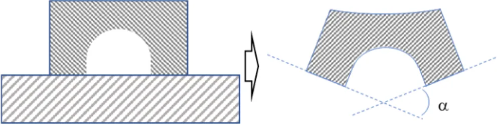
Material Ti-6AI-4V is used. Parameters are defined in Yannick Robert’s works |12]. We use two types of models. The first one is a 10x10x10 mm cube (figure 2), meshed with 1mm size hexahedral elements. The second is the bridge model (figure 3) as described in Kruth’s work [13] and meshed with 1 mm large and 0.5 mm thick hexahedral elements.

To validate our approach we’ll use the Bridge Curvature Method (BCM). A bridge (figure 3) is built on a plate and then cut off after printing. The resulting spring-back effect is then measured thru the angle between the bottom surfaces of the two bridge’s pillar bridge (figure 4). Measured angles given in Kruth’s works [13] are compared with our numerical results.

Figure 3. Bridge model for quantitative validation as described by Kruth [13]

Figure 4. Measured angle after spring back

Table 1. KUL-SLM machine parameters used to build Ti-6Al-4V test parts.

Hach spacing 74 µm

Scan speed 225 m/s

(11)

IC-MSQUARE 2020

9

Laser power 42 W

Layer thickness 30 µm

4.2. Influence of the temperature dependency of the thermal conductivity

We apply the “by layer” approach described above on the cube model. We can observe in figure 5 that the first temperature peak is the same with and without the temperature dependency. Differences appear from the second peak. This can be explained by the higher conductivity of the previously activated layers, when the temperature dependency is set for this parameter. This layer is re-heated at each new activation of the upper layers. The heat flow, from the top to the bottom, between two consecutive layers is then greater. As a result, the cooling rate is higher which can be observed on the decreasing slop of the curve after each peak.

4.3. Influence of the laser scanning path

We apply the ‘by hatch’ activation strategy on the cube model first. Temperature evolution of the 6th

layer is then compared with the ‘by layer’ approach.

As shown in figure 6, the heat peaks are slightly higher with the activation ‘by hatch’ than ‘by layer’. This can be explained by the shorter time between two sequences of activation for the former strategy

.

Figure 5. Temperature evolution, with and without conductivity dependency with temperature, in the 6 th_{layer of the cube model.}

Figure 6. Comparison of the temperature evolution in the 6 th_{layer of the}

(12)

IC-MSQUARE 2020

as explained in the chapter 2. The previously activated elements are still at a high temperature when the next range of elements is activated which was not the case for the “by layer” strategy. As a result, the maximum temperature reached is also higher for the “by hatch” strategy (table 2).

Table 2. Maximal temperature depending on the strategy for Tia6v on 10x10x10 cube

Scanning strategy Tmax (K)

By Layer 1911

By Hatch along x 2122

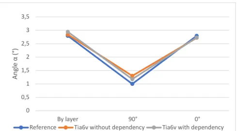
Using the BCM, we can compare the angle given by the simulation with the experimental values. In the figure 7 we can see that the precision earned depends both orientation and activation strategy.

We can observe that the accuracy of the “by layer” strategy is not improved by the temperature dependency of the conductivity whereas the gain for the “by hatch” strategy rises to 12%. The former modelling is too coarse to capture this level of details whereas the latter introduces a temporality in the activation sequence within the layer which allows the change in the laser orientation to be captured.

Table 3. Comparison of the angle depending on the strategy Scanning

strategy Reference No dependency With dependency Gain of accuracy % By layer _2.797 _2.841 _2.945 _-3.7 90° 1 1.3 1.1775 +12.3 0° 2.797 2.723 2.73 +0.25 5. Conclusion

In this work, a macroscopic model for the thermo-mechanical simulation of additive manufacturing has been developed. Thermal dependency of specific heat and conductivity parameters has been added.

0 0,5 1 1,5 2 2,5 3 3,5 By layer 90° 0° An gl e α (° )

Reference Tia6v without dependency Tia6v with dependency

Figure 7. Comparison between the measured reference angle, depending on the scanning strategy, with the numerical results with and without depending temperature dependency for the conductivity

(13)

IC-MSQUARE 2020

11

Element activation/deactivation technique is used. Two element activation strategies have been studied. The BCM method was used to compare the results. Good agreements between the measured angles and the simulation results for Tia6v material and two scanning strategies at 0° and 90°, were found. Thanks to this work, the cooling history is handled with more accuracy in AM simulation. This will allow to introduce phase transformation in the numerical model for which the cooling rate is a first order parameter. We also demonstrate that a more realistic element activation sequence improves a lot the results. These models will be enhanced with more detailed in future works. At last, meso-scale modelling will be also explored to better calibrate the heating energy to improve again the results.

6. References

[1] Lindgren L-E and Hedblim E, Commun. Num. Meth. Eng., 17(9), 647-57 [2] Michaleris P, Fin. Elem. Anal. Des., 86, 51-60

[3] Chiumenti M, Neiva E, Salsi E, Cervera M, Badia S, Moya J, Chen Z, Lee C and Davies C, Commun. Num. Meth. Eng., 18, 171-85

[4] Gusarov A V and Kruth J-P, Int. J. Heat Mass Trans., 48(16), 3423-34 [5] Hodge N E, Ferencz R M and Solberg J M, Appl. Surf. Sci., 254(4), 975-9 [6] Li J F, Li L and Stott F H, Int. J. Heat Mass Trans., 47(6-7), 1159-74 [7] Chen Q, Guillemot G, Gandin Ch-A and Bellet M, Add. Manu., 16, 124-37

[8] Denlinger E R, Heigel J C and Michaleris P, Proc. Inst. Mech. Eng., B: J. Eng. Manu., 229(10), 1803-13

[9] Zhang Y, Guillemot G, Bernacki M and Bellet M, Comp. Meth. Appl. Mech. Eng., 331, 514-35 [10] Bugatti M and Semerato Q, Add. Manu., 23, 329-46

[11] Chen Q., Beauchesne E., Arnaudeau F., Dahoo P.-R., Meis C., Model. of mech. behave. in add. manuf. at part scale, J. of Physics: Conf. Series, Vol. 1391, 8th Int Conf. on Math. Model. in Phys. Science 26–29 Aug. 2019, Bratislava, Slovakia

[12] Robert Y., Sim. num. du soud. du ta6v par laser yag impuls. Phd Thesis. Sept 2007. Ecole Des Mines-Paritech

[13] Kruth J-P, Deckers J., Yasa E., Wauthlé R., Assess. and compar. Influenc. Fac. of res. stresses in S.L.M. Proceedings of the Institution of Mechanical Engineers Part B Journal of Engineering Manufacture (P I MECH ENG B-J ENG)