The Swiss Alpine glaciers’ response to the global ‘2 °C air temperature target’
This article has been downloaded from IOPscience. Please scroll down to see the full text article. 2012 Environ. Res. Lett. 7 044001
(http://iopscience.iop.org/1748-9326/7/4/044001)
Download details:
IP Address: 134.21.47.136
The article was downloaded on 05/02/2013 at 08:45
Please note that terms and conditions apply.
View the table of contents for this issue, or go to the journal homepage for more
Environ. Res. Lett. 7 (2012) 044001 (12pp) doi:10.1088/1748-9326/7/4/044001
The Swiss Alpine glaciers’ response to the
global ‘2
◦
C air temperature target’
Nadine Salzmann
1, Horst Machguth
2,3and Andreas Linsbauer
21University of Fribourg, Department of Geosciences, Alpine Cryosphere and Geomorphology Group, Chemin du Mus´ee 4, 1700 Fribourg, Switzerland
2University of Zurich, Department of Geography, Glaciology and Geomorphodynamics Group, Winterthurerstrasse 190, 8057 Zurich, Switzerland
3Geological Survey of Denmark and Greenland (GEUS), Marine Geology and Glaciology, Ø Voldgade 10, DK-1350 Copenhagen, Denmark
E-mail:[email protected]
Received 11 July 2012
Accepted for publication 13 September 2012 Published 1 October 2012
Online atstacks.iop.org/ERL/7/044001 Abstract
While there is general consensus that observed global mean air temperature has increased during the past few decades and will very likely continue to rise in the coming decades, the assessment of the effective impacts of increased global mean air temperature on a specific regional-scale system remains highly challenging. This study takes up the widely discussed concept of limiting global mean temperature to a certain target value, like the so-called 2◦C target, to assess the related impacts on the Swiss Alpine glaciers. A model setup is introduced that uses and combines homogenized long-term meteorological observations and three ensembles of transient gridded Regional Climate Model simulations to drive a distributed glacier mass balance model under a (regionalized) global 2◦C target scenario. 101 glaciers are analyzed representing about 50% of the glacierized area and 75% of the ice volume in
Switzerland. In our study, the warming over Switzerland, which corresponds to the global 2◦C target is met around 2030, 2045 and 2055 (depending on the ensemble) for Switzerland, and all glaciers have fully adjusted to the new climate conditions at around 2150. By this time and relative to the year 2000, the glacierized area and volume are both decreased to about 35% and 20%, respectively, and glacier-based runoff is reduced by about 70%.
Keywords: glacier, RCM, mountain, 2◦C target
S Online supplementary data available fromstacks.iop.org/ERL/7/044001/mmedia
1. Introduction
There are many unknowns and uncertainties associated with the changes in the climatic system and the related impacts. Among the few international consensuses is the global mean air temperature increase during the past decades and its very likely continuation in the coming decades (IPCC2007). The ongoing debate on how to limit climatic change and related
Content from this work may be used under the terms of the Creative Commons Attribution-NonCommercial-ShareAlike 3.0 licence. Any further distribution of this work must maintain attribution to the author(s) and the title of the work, journal citation and DOI.
impacts focuses mainly on a ‘2◦C air temperature target’, described as the maximum allowable warming to avoid dangerous anthropogenic interference in the climate (Randalls 2010). The warming is understood as an increase in mean global air temperature relative to the pre-industrial level (den Elzen and Meinshausen 2006, Meinshausen et al 2009).
Although such target concepts imply to be a clear goal for politicians and decision makers, there are several remaining issues from a scientific perspective, including (i) the analog application of a global air temperature target on a regional level, and (ii) the effective impacts of a
Environ. Res. Lett. 7 (2012) 044001 N Salzmann et al
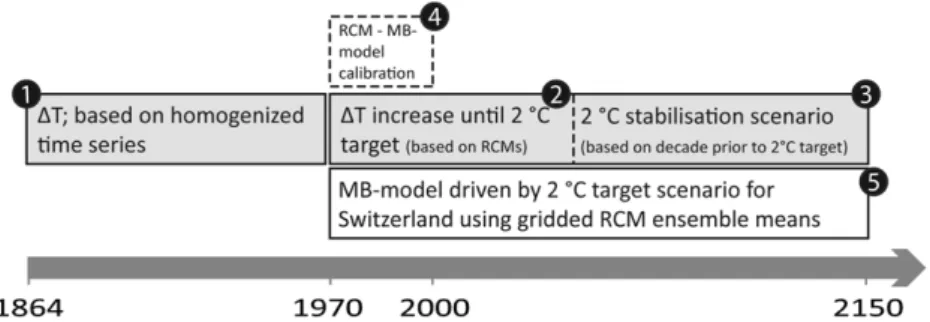
Figure 1. Schematic of the applied approach to construct the 2◦
C target time series for Switzerland and to simulate the related response of the Swiss glaciers.
defined target on a specific environmental system. Regarding (i), the global target concept is complicated by the fact that observed air temperature trends show significant spatial variation. While the global trend of mean air temperature increase is clear (Trenberth et al2007), there are significant regional differences in their magnitude observed (Jones and Moberg 2003). For average global surface air temperature, a trend of about +0.08◦C/decade is observed between 1901–2005 (Trenberth et al 2007), whereas for instance for the European Alps and Switzerland, higher trends of about +0.1◦C/decade are reported (based on the period
1901–2000) (Begert et al2005). Concerning (ii), it must be considered that the effective impacts of climate change on a specific environmental system do not only depend on changes in air temperature, but also on other climate variables.
Mountain glaciers are among the most sensitive environmental systems to climatic changes because of their proximity to melting conditions (Haeberli and Beniston 1998, Oerlemans 2001). Moreover, mountain glaciers often play a key role in the socio-economic system of mountain regions and the adjacent lowland by serving as fresh water source and by controlling in some regions a great part of the hydrological cycle (Barnett et al 2005, Kaser et al 2010). Therefore, the globally observed negative glacier mass balance trends (WGMS 2009), the unrestrained retreat of glacier tongues (WGMS2009), and the projected continued warming as consistently simulated by climate models (IPCC 2007) are of major concern. Relative to the present, glacier area and fresh water supplied by glacier melt will very likely be considerably reduced in a 2◦C warmer climate and significantly affect societies (Barnett et al2005, Collins2008, Kaser et al 2010). Plausible regional impact scenarios are thus needed to better understand the effects of global climate change on regional-scale systems and eventually to serve as a basis for the development of adequate adaptation measures.
The objective of this study is to introduce a modeling setup that enables the assessment of the impacts of a defined global mean air temperature target on a regional-scale system. As an example, we take up the ‘2◦C target’ to simulate the related impacts on the Swiss Alpine glaciers. The aim is to use and combine observational data and the latest climate and glacier mass balance models to provide outcomes for an entire mountain area at a very high level of detail, including results for glacier extent, volume and runoff, and insight to the models’ performances.
2. Data, models and methods
The modeling setup of our approach is described in the following sections and may be divided into five major steps (see figure 1). First (1), the air temperature change for Switzerland is estimated from 12 homogenized time series for the period before 1970, which is the starting point of the initialization period (1970–2000) of the mass balance (MB) model in this study. Second (2), the 2◦C target for Switzerland is defined as the point in time when the decadal mean temperature (determined based on transient Regional Climate Model (RCM) data) has changed by 2◦C relative
to the 1970s. In order to enable all glaciers to reach a new equilibrium, in a third step (3) we prolong and stabilize the scenario time series after the point in time where a 2◦C warming was reached until 2150 by adding randomly 2-year packages from the ultimate decade before the 2◦C target was reached. Fourth (4), the glacier mass balance model is calibrated for the time span 1970–2000 against observed glacier mass balance data and driven by downscaled and de-biased RCM output. Fifth (5), the calibrated glacier mass balance model is driven by downscaled and de-biased gridded transient RCM data until the 2◦C target is reached, and is then continued under stabilized 2◦C target conditions until 2150, in order to enable all glaciers to reach a new equilibrium. 2.1. Observed air temperature change for Switzerland between 1880 and 1970
For the determination of the past air temperature change for Switzerland relative to the pre-industrial level, we used 12 homogenized monthly mean air temperature series since 1880 (see Begert et al 2005). The mean value of these 12 stations represents the main characteristics of the temperature evolution for all areas of Switzerland (Begert et al 2005). Also Ceppi et al (2010) found only small spatial variability for annual air temperature trends within Switzerland in their study, where a 2 km × 2 km gridded data set based on 91 homogenized time series from 1959 to 2008 was used. However, Ceppi et al (2010) and Appenzeller et al (2008), both report on a slight dependency of the air temperature trend on altitude. In the present study, possible altitude dependence is partly considered via the de-biasing of the RCM results (see section2.4), which is based on 14 high-elevation stations and on the time period 1979–2010. Hence, de-biasing is focused
on high mountain terrain where most of the glacier area is located.
The air temperature increase between 1880 and 1970 was determined by calculating a 30 yr mean change (1955–85 minus 1865–95) from the 12 homogenized time series. We found an air temperature increase of about 0.5◦C, which is consistent with mean decadal and centennial changes reported by other studies for the European Alpine region (Begert et al 2005, Brunetti et al 2006, Auer et al 2007, Rebetez and Reinhard 2007) and probably does not deviate much from the resulting change when using 1850–80 as the initial 30 yr mean.
2.2. RCM-based simulation of the 2◦C target scenario In order to generate the 2◦C target scenario for Switzer-land, we used seven transient RCM simulations at monthly temporal resolution from the EU-ENSEMBLES program (van der Linden and Mitchell 2009) (see sup-plementary material S1 available at stacks.iop.org/ERL/7/ 044001/mmedia) for the grid cells over Switzerland plus some neighboring cells to better represent the Alpine arc (see supplementary material S2 available at stacks.iop.org/ ERL/7/044001/mmedia). We assume that ensemble means are more plausible scenario guesses than single simulations (e.g. Guo et al 2007, Thomson et al 2006). Consequently, from the seven RCM simulations we built the following three ensembles by averaging monthly mean temperature and precipitation over all ensemble members in order to drive the mass balance model: (1) an ensemble including all seven RCM members (E7m), (2) an ensemble involving the four ECHAM5-r3 driven RCM simulations (E4m), and (3) a ‘mini’-ensemble comprising two RCM runs driven by two different experiments of the GCM HadCM3Q (E2m). E7m is the most complete ensemble, however, at the cost of averaging three different driving GCMs (see supplementary material S1 available at stacks.iop.org/ERL/ 7/044001/mmedia) leading to a possible underestimation of climate variability. E4m is considered the base scenario in our study because of a consistent GCM forcing at a still reasonable number of ensemble members. Finally, for E2m, the number of members is at the lowermost limit and it is driven by two different experiments using the same GCM (see supplementary material S1 available at stacks.iop.org/ ERL/7/044001/mmedia) that may cause inconsistency similar to E7m. Nevertheless, E2m is included in this study because its temperature evolution clearly differs from the other two ensembles and the +2◦C target is reached much earlier (see below) and provides thus the possibility to study the impacts of fast warming followed by a long period of stable temperatures.
The 2◦C target is then determined per ensemble as the time when the decadal mean has changed by 2◦C compared to the 1970s. That is, for Switzerland we allow a total increase of 2.5◦C (0.5◦C between 1880 and 1970, +2◦C since 1970) based on the ratio between the reported (see section 1) higher decadal changes for the European Alps and Switzerland (0.1◦C/decade) compared to the global
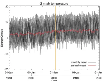
Figure 2. RCM-based air temperature time series for the 2◦C target from 1970 until 2150 for E4m as a mean of all grid boxes above 2000 m a.s.l. in Switzerland (see also supplementary material S2 available atstacks.iop.org/ERL/7/044001/mmedia). The orange line marks the period where the 2◦
C target is reached.
mean (0.08◦C/decade) changes. In this manner, we account for the above mentioned observed higher warming trends in Switzerland compared to the global mean, which we assume to continue. We base our assumption (i) on the spatial pattern shown by the MIP3 GCM projections, which indicate enhanced future warming for central Europe (Meehl et al2007), and (ii) on the plausibility in view of occurring changes in albedo caused by glacier and snow area reduction as a result of the warming trends and thus forcing the positive ice-albedo feedback. Like this, the 2◦C target for Switzerland is reached at about 2045 (E7m), 2055 (E4m) and 2030 (E2m). To allow all glaciers to adjust to the new climate conditions, the simulation is continued until 2150 based on the RCM simulation of the last decade prior to the 2◦C target (2040–50 (E7m); 2050–60 (E4m) and 2025–35 (E2m)). From these decades one year is randomly picked, and the RCM grids from this year and from the following year are then appended to the first part of the scenario time series. The process is repeated for all years until 2150. We have chosen this approach because to our knowledge, there are no RCM runs available yet that provide simulations until 2150 under stabilized 2◦C target conditions. This approach leads to plausible interannual variability as shown in figure 2. Appending randomly chosen two-year time windows might result in the suppression of natural climate cycles (e.g. North Atlantic Oscillation). However, choosing longer time windows, which create repeated cycles of increasing air temperature followed by an immediate drop due to the strong increasing trend in air temperature in the middle of the 21st century, hinders in our model setup (only glacier retreat is addressed) the stabilization of glaciers at a realistic extent.
In order to better assess the influence of the 2◦C target, we additionally run the mass balance model by the fully transient RCM output for 1970–2098 (i.e., no stabilization after the 2◦C target has been reached) for all the three
Environ. Res. Lett. 7 (2012) 044001 N Salzmann et al
ensembles. Calibration (see section2.4) is identical to the 2◦C scenario runs.
2.3. Glacier mass balance simulation
The glacier mass balance is calculated using a distributed mass balance model (MB-model) that is fully described in Machguth et al (2009). The MB-model is a simplified energy balance model, which runs at daily steps and uses gridded RCM data of 2 m air temperature, precipitation (P) and total cloudiness (n) for input. Cumulative mass balance bc on day t + 1 is calculated for every time step and over
each grid cell of the Digital Terrain Model (DTM) according to Oerlemans (2001): bc(t + 1) = bc−t ( 4t(−Qm)/lm+Psolid if Qm > 0 Psolid if Qm≤0 (1) where t is the discrete time variable,1t the time step, lmthe
latent heat of fusion of ice (334 kJ kg−1) and Psolid the solid
precipitation in meter water equivalent (m w.e.). The energy available for melt (Qm) is calculated as follows:
Qm=(1 − α)Sin+C0+C1T (2)
whereα is the surface albedo (three constant albedo values are applied: snow = 0.72, firn = 0.45 and ice = 0.27) and Sin the incoming shortwave radiation at the surface. For
T (air temperature), the unit is ◦C, and C
0 +C1T is the
sum of the longwave radiation balance and the turbulent exchange (Oerlemans 2001). C1 is set to 12 W m−2 K−1
and C0 is tuned to −45 W m−2 (cf Machguth et al 2009).
Accumulation equals Psolid, redistribution of snow is not taken
into account and a threshold range of 1 to 2◦C is used to distinguish between snowfall and rain. Any melt water occurring on the updated glacier perimeter (see section on glacier-retreat parameterization) is considered as runoff.
Simplifications in the MB-model (e.g. debris cover is not considered) limit the number of glaciers, where reasonable mass balances can be calculated (Machguth et al2009). As a result, glacier mass balance and retreat scenarios are restricted to 101 Swiss Alpine glaciers, representing about 50% of the total glacier area and about 75% of the total ice volume in Switzerland.
Glacier retreat is simulated based on the modeled mass balances and the 1h glacier-retreat approach (Huss et al 2010b). The latter parameterizes glacier surface elevation change by distributing glacier mass loss or mass gain to the entire glacier surface according to altitude dependent functions of previously observed change in glacier thickness. Here, we use the 1h functions as proposed for the Swiss Alps (Huss et al2010b). Glacier geometry is updated annually based on calculated surface elevation changes. Glacier surface mass balance is calculated on updated topography and thus considers the mass balance height feedback, i.e. a reduction in glacier thickness implies warmer air temperatures due to a lower elevation of the glacier surface and consequently a more negative mass balance. The initial glacier extent is given by
the glacier outlines from 1973 (M¨uller et al1976) and a 25 m resolution DTM (Digital Terrain Model, resampled to 100 m) from Swisstopo (Swiss Federal Office of Topography), which refers to the glacier surfaces at mid-1980s. Glacierized grid cells are forced to become ice-free when their elevation falls below the elevation of the glacier bed.
Glacier ice volume is derived from estimated glacier ice thickness and modeled bed topography. The calculation of the ice thickness is based on the assumption of perfect plasticity (cf Paterson 1994) and is fully described in Linsbauer et al (2012). Ice thickness is estimated at points along major central branch lines using an estimated average basal shear stress (τ) per glacier, based on an empirical relation between τ and glacier elevation range set up by Haeberli and Hoelzle (1995). The ice thickness variability (h) for individual glacier parts is governed by the zonal surface slope (s) of 50 m elevation bins along the branch lines,
h = τ
fρg sin s (3)
whereτ is the basal shear stress, f the shape factor (0:8), ρ the ice density (900 kg m−3) and g the acceleration due to gravity (9.81 m s−2). This implies thin ice, where the glacier surface is steep, and thick ice, where it is flat. Finally, ice thickness is interpolated from the estimated point values and bed topography is derived by subtracting the distributed ice thickness estimations from the surface DTM.
The model used in this study to estimate the ice thickness distribution was validated with ground penetrating radar (GPR) measurements (Linsbauer et al 2012) and compared to GPR-calibrated estimates from Farinotti et al (2009). The evaluation revealed that the method used in this study simulates the parabolic shape of glacier beds in good agreement with the shape of the GPR measurements, and that the measured and modeled ice thickness values are within an uncertainty range of ±30%. The ice volume estimates from Farinotti et al (2009) are about 20–30% higher for individual, and about 10% higher for the sample of all Swiss glaciers, probably due to the stronger smoothing of the approach by Farinotti et al (2009) that indicates higher basal shear stresses. Nevertheless, the overall structure of the ice thickness distribution reflects a very similar picture in both studies and the found numbers are in the range of expected uncertainties.
2.4. Downscaling, de-biasing and application of gridded RCM time series to the MB-model
The MB-model runs at daily temporal resolution and therefore daily time series of RCM fields are in principle the favored model input. However, we found some unrealistically high spatial and temporal variability in the daily RCM fields (see below), which did not allow the application of a general, domain-wide de-biasing procedure. Therefore, we used monthly fields, which showed considerably improved patterns, and downscaled them to daily time series by linear interpolation. In combination with a calibration procedure (see below), in the model-set up precipitation occurs with a frequency of five days, while the monthly sums from the RCM
data are preserved. These kind of approaches are commonly used for glacier mass balance models when dealing with input data at a coarser temporal resolution than the model resolution (e.g. Oerlemans and Hoogendorn1989).
The gridded 25 km spatial resolution RCM fields furthermore need to be downscaled to the MB-model’s resolution of 100 m. This downscaling is implemented in the MB-modeling setup and is thus directly applied to each RCM grid cell while the model is running. The method is summarized in the following and a more detailed description may be found in Machguth et al (2009). RCM T grids are downscaled by means of inverse distance weighting (IDW) interpolation and by the use of a vertical lapse rate value (0.0065◦C m−1), while cloudiness is interpolated through
IDW, only. Potential clear sky short wave radiation (Sin,clear)
for the 365 days of the year is calculated prior to the model run. During the model run, the corresponding Sin,clear is
corrected for attenuation of clouds (τcl). For this, we used the
downscaled fields of n and calculatedτcl after Greuell et al
(1997). Precipitation is downscaled by multiplying the RCM grids with a high-resolution scaling array, which is calculated by multiplying mean annual RCM P for 1971–90 with the gridded (2 km × 2 km) precipitation climatology (1971–90) of Schwarb et al (2001).
The de-biasing of the RCM fields is done for each grid cell and each variable according to the method described in Machguth et al (2012). For T and Sin, the de-biasing is
based on 14 high-elevation stations and achieved as follows (cf Machguth et al 2012 for details). From the grid cells that are located at the 14 weather stations (the difference in altitude between grid cell and weather station is adjusted) a mean bias in T is calculated for every day of the year (averaged over 1970–2010). During the actual model run, all temperature values (at 100 m spatial resolution) are corrected by the corresponding daily bias. Observed cloudiness (nobs)
is calculated from observed Sin according to Greuell et al
(1997) and cloudiness from the RCM is adjusted to meet nobs
by means of cumulative density function matching (Machguth et al2012). Corrections are temporally and spatially uniform, which guarantees that the spatial pattern as given by the RCM (e.g. warmer T in the south and at lower elevations) and trends (which can differ among the regions or elevations) are preserved. For precipitation, the climatology of Schwarb et al (2001) is directly used for the precipitation scaling (see the following section) because to our knowledge, this is currently still the best available precipitation climatology data set for Switzerland.
The accuracy of the downscaled fields is limited as knowledge of real meteorological conditions at the glacier sites is imperfect. In particular the large uncertainties in observed high mountain precipitation (Sevruk 1997) hamper the de-biasing procedure and makes it impossible to achieve a level of data accuracy that would allow the calculation of accurate mass balances for each individual glacier. We have approached these limitations by applying a calibration procedure, where the MB-model is driven by the downscaled and de-biased RCM time series for the period 1970–2000 and precipitation is calibrated for each glacier
individually in order to achieve a prescribed cumulative mass balance (Machguth et al 2012). Prior to the calibration of precipitation, the mass balance model is adjusted to meet observed summer mass balance as described in Machguth et al (2009, 2012). The term ‘calibration of precipitation’ is used here to distinguish from de-biasing. While the latter is based solely on comparing meteorological observations and RCM data, calibration of precipitation involves the mass balance model with its uncertainties (cf Machguth et al2008) as well as uncertainty in the determination of the observed mass balance (see below). Here, we have applied precipitation calibration factors ranging from 0.19 to 1.2 (E2m), 0.11 to 1.12 (E4m) and 0.11 to 1.09 (E7m) with respective average/median of 0.62/0.56 (E2m), 0.48/0.45 (E4m) and 0.49/0.46 (E7m), in order to achieve a prescribed cumulative mass balance. As shown in Machguth et al (2012), when using the precipitation climatology of Schwarb et al (2001) instead of RCM data, a mean correction factor of 1.18 has to be applied. This factor is in line with the suggested correction of the uncorrected (i.e. undercaught) precipitation climatology (cf Schwarb et al 2001). The fact that the precipitation climatology requires much smaller adjustment than the three RCM ensembles indicates that the latter do considerably overestimate precipitation in high mountain areas of the Swiss Alps. Hence, it appears reasonable to assume that the calibration procedure mainly corrects for biases in the RCM data and to a lesser degree for inevitable uncertainties in the mass balance model and the prescribed cumulative mass balance. The latter is established from the mean observed cumulative mass balance of nine Alpine glaciers (Zemp et al2008) and 50 Swiss glaciers, calculated by a combined method of modeling and observations (Huss et al 2010a, 2010c). Because for most of the 101 selected glaciers no individual observational records are available, we prescribed for all glaciers an identical cumulative mass balance of −11 m w.e. for the calibration period, which represents about a mid-value to the diverting cumulative mass balances reported by Zemp et al (2008) and by Huss et al (2010a, 2010c) (cf figure 4(a)). The downscaled, de-biased and precipitation-calibrated RCM data are subsequently used to run the MB-model for the scenario period.
The MB-model contains simplifications and there is considerable uncertainty in the model input. First and foremost, the influence of using the three RCM ensembles (cf section 2.2) was evaluated by performing for each ensemble the 1970–2000 calibration (−11 m w.e.), and based on the latter a 1970–2150 scenario mass balance run. An additional straightforward sensitivity assessment was then performed for E4m to evaluate the sensitivity to the following sources of uncertainties:
(a) Mean observed cumulative mass balance (1970–2000) according to Zemp et al (2008) and Huss et al (2010a, 2010c) deviate clearly (cf figure 4(a)). Therefore, in addition to applying the value −11 m w.e. for prescribed cumulative mass balance, we performed two more model calibrations using the values −9 m w.e. and −13 m w.e., respectively.
Environ. Res. Lett. 7 (2012) 044001 N Salzmann et al
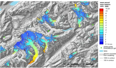
Figure 3. Modeled mean annual mass balance distribution 1970–2000 for a selected region (Bernese and Valais Alps) for the E4m, calibrated to an intermediate mass loss of −11 m w.e.
(b) There is a large spread found among the 1h functions of individual glaciers (Huss et al 2010b). Consequently, we performed two additional model runs with modified 1h functions, indicating (i) a more pronounced mass loss at the tongue (active glacier retreat), and (ii) a more concentrated thinning at the ELA (‘down wasting’ Paul et al2004).
(c) The third test is performed to account for albedo lowering associated with glacier retreat (e.g. Oerlemans et al2009). Instead of using a constant ice albedo of 0.27 during the entire scenario simulation, we gradually lowered the ice albedo to 0.17 during the first 20 yr of the scenario period (2000–20) and hold it constant afterwards.
(d) The assumption of identical mass balances (1970–2000) for all glaciers contrasts to the findings of Paul and Haeberli (2008) and Huss et al (2010a) who found more negative mass balances for the largest glaciers. Thus, we calculated observed glacier mass balances (adjusted to a mean of −11 m w.e. for all 101 glaciers) as a function of glacier size, based on the data from Paul and Haeberli (2008). The size dependent mass balances for the individual glaciers were then applied to an additional model calibration.
3. Results
The mean annual mass balance distribution for the calibration period after the de-biasing and the calibration (for −11 m w.e.) for a selected area (Bernese and Valais Alps) is shown in figure3. The cumulative mass balance of all 101 glaciers (−11 m w.e.) 1970–2000 is shown in figure4(a). The comparison of the interannual variability of mass balance from E4m (figure 4(b)) with values reported by Huss et al (2010a, 2010c) shows the mean values of the mass balance data achieved over a 30 yr period based on the GCM-driven RCM simulations. The latter are independent of real meteorological conditions and thus the observed pattern of year-to-year variability in mass balance cannot directly be compared
to the model results. However, statistical properties over climatological time scales (30 yr) can be compared: modeled cumulative mass balance shows a plausible course with less and more negative periods as also found in the observations (figure4(a)), and the magnitude of interannual variability of mass balance (figure 4(b)) is in the range of the observed values, although slightly underestimated in winter.
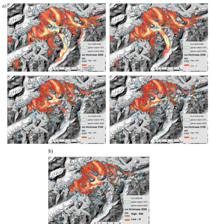
The resulting glacier extent for the Aletsch area, which encompasses the largest glacier of the Alps (Aletsch glacier), is shown in figure5under the 2◦C target scenario (E4m) at four time steps (2000, 2050, 2100 and 2150), and without a 2◦C stabilization (E4m) at time step 2098 (b). Glacier retreat until 2150, 2100 and 2098 respectively, is obvious in both cases, as well as the considerable decreases in ice thickness, particularly in the ablation areas. Furthermore, the effect of the 2◦C stabilization is evident, particularly for the raise of the ELA but also for ice thickness. In the stabilization scenario, the ELA does not move upwards any further between 2100 and 2150 (and thus remains below the ELA elevation without a +2◦C stabilization at 2098), while ice thickness is still decreasing as part of the delayed glacier response. The annual mass balances (E4m) for the Aletsch (87 km2in 1973) and nearby Lang (9.6 km2in 1973) glaciers are shown in figure6 (the two glaciers are marked ‘A’ and ‘L’ in figure5(a)). There is a negative trend until around 2055, that is, where the 2◦C
target is reached. After 2055, the trend in mass balance reverts. The small Lang glacier adjusts faster than the large Aletsch glacier and reaches a new equilibrium at around 2090. The Aletsch glacier is just about to reach a new equilibrium at the end of the model simulation period at 2150.
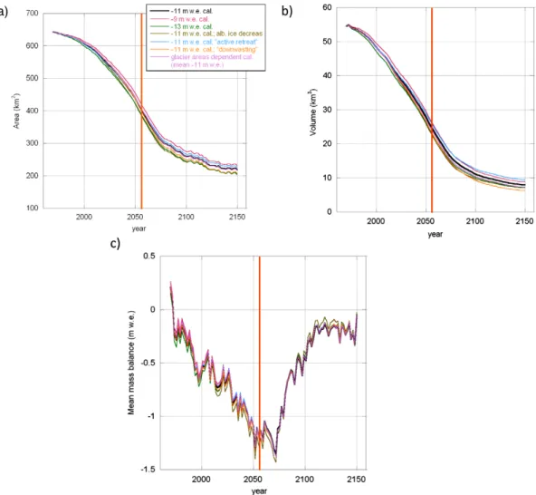
Glacier volume and glacier area begin to stabilize around 2100 (E4m) at about 20% for volume and at about 35% for area, relative to the values of the year 2000 (figures 7(a), (b)). Comparing these numbers to the results achieved by E4m without a +2◦C stabilization (figures 8(a), (b)) it is
evident that the glaciers do not stabilize either, resulting in a significant larger ice loss (area and volume). Mean mass balance of all 101 glaciers (figure 7(c)) shows an increase after 2055 that is intermediate to the behavior of Lang and
Figure 4. (a) Comparison between cumulative mass balance for the 101 glaciers based on the RCM ensembles means (E7m, E4m, E2m), calibrated with −11 m w.e., and the values from Zemp et al (2008) and Huss et al (2010a,2010c). (b) Comparison between yearly values of annual, summer and winter balance for E4m and Huss et al (2010a,2010c).
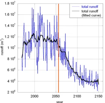
Aletsch glacier (figure 6). The ELA is shifting up mainly during the first half of the 20th century, and remains relatively stable afterwards (figure 5). The calculated changes result furthermore in a reduction of glacier-based hydrological run off (figure9) by about 65–70% for E4m.
In terms of sensitivities, the straightforward assessment (figure7) indicates that the sensitivity to the albedo lowering is about similar to a more negative (−13 m w.e.) prescribed cumulative mass balance. The effect of varying the 1h functions doubles albedo and calibration sensitivity. The influence of a glacier-size dependent mass balance calibration is negligible. Comparing the result of the sensitivity analysis and the influence of the choice of the ensembles (without +2◦C stabilization), it becomes clear that the uncertainty from the RCM scenarios is the largest uncertainty source
and by applying a +2◦C stabilization scenario, much of the uncertainty stemming from the driving RCM data is reduced.
4. Discussion and conclusions
This study presents an approach that combines homogenized long-term observations and latest transient gridded RCM simulations to drive a distributed MB-model in order to assess the impacts of a global 2◦C air temperature target on Swiss Alpine glaciers. With the modeling setup, the considered input data in form of entire RCM grids, the included feedback processes (e.g. the mass balance surface height feedback) and the generated detailed output data for a large number of
Environ. Res. Lett. 7 (2012) 044001 N Salzmann et al
Figure 5. (a) Area and ice thickness change for the glaciers of the Aletsch region under a 2◦C target scenario (E4m) and the ‘−11 m w.e. calibration’ for four different points in time and (b) without +2◦C stabilization for 2098. Glacier outlines for 1973 are in gray and for the year 2000 in blue. The decadal mean ELA is in green. Glacier areas in light blue have not been modeled.
glaciers, we intended to use and combine most recent data and methods currently available in an innovative approach.
Based on the here applied 2◦C target scenario, we found a significant decrease of glacier extent and volume, with a related reduction of a glacier-based hydrological runoff in the order of 65–70% (figure 9) relative to the present. The effect of stabilizing the scenario once the 2◦C target is reached is evident (figures5 and8). Although the numbers resulting for the 2◦C target scenario already indicate possible severe impacts on temporal water availability for sectors like hydro-power production or agriculture, the 2◦C
target scenario is probably relatively conservative. Latest observations of global CO2 emissions and air temperature
increase indicate that the 2◦C target maybe reached earlier in time than projected by current climate models and that stabilization at +2◦C will not be met (Parry et al 2009). Furthermore, we have used the A1B scenario, which is at the upper end of the projections but less negative than for example the A2 scenario path. However, since most of the different scenario paths start deviating considerably only at around 2050 (Trenberth et al 2007), that is, where we have indicated the 2◦C target in our study, the results for a +2◦C
Figure 6. Annual mass balances for the two glaciers ‘Aletsch’ (A) and ‘Lang’ (L) for the E4m and −11 m w.e. calibration. The orange line marks the period where the 2◦
C target is reached.
stabilization scenario would probably not deviate much from our results. The applied straightforward sensitivity assessment for the calibration period (1970–2000) furthermore showed rather low deviation ranges of about 15% for final ice volume and 5% for final glacier area. Since we only addressed selected sources of uncertainties, it is clear that these values would likely be larger in a more comprehensive analysis (cf figures 7and8).
From a glacier modeler’s perspective, the simulation of a target and stabilizing scenario is as such a valuable experiment. It offers insights into the model’s performance that go beyond the specification of glacier mass loss. In the MB-model, the bulk of small to mid-sized glaciers adjust for instance to the new climate conditions approx. 40 yr after the 2◦C target was reached, while this has taken about 100 yr for the largest glaciers. Both of these numbers correspond well with previous studies on glacier response times (e.g. Haeberli and Hoelzle1995, Bahr et al1998). Our study includes 101 glaciers, which correspond to about 50% of ice area and 75% of ice volume. The remaining glaciers are not included because they are for example debris covered, which modifies the energy fluxes at the glacier–atmosphere interface in a way that is not considered in the MB-model. Debris covered ice
a)
Figure 7. Temporal evolution of area (a), volume (b) and mass balance (c) for the 101 Swiss glaciers for E4m, including the sensitivity assessment (fitted curves). The orange line marks the period where the 2◦
Environ. Res. Lett. 7 (2012) 044001 N Salzmann et al
Figure 8. Temporal evolution of area (a), and volume (b) with and without a +2◦C stabilization for E7m, E4m and E2m (fitted curves).
Figure 9. Total runoff for the 101 glaciers for E4m (−11 m w.e. calibration), annual values (fitted curve). The orange line marks the period where the 2◦
C target is reached.
will vanish at slower rates than exposed ice but nevertheless it is difficult to assess if the relative mass loss of the excluded glaciers will be larger or smaller than for the modeled ones. Very small glaciers are also excluded and they are likely to disappear early, possibly compensating for the lower melt rates of debris covered ice.
Finally, the study discloses several remaining issues and challenges from a scientific point of view that need to be further addressed. Although the simulated interannual variability (figure 4(b)) is plausible, the biases and the uncertainties in the RCM data over complex mountain topography remain a major impediment when applying
RCM data to impact models. In this study, we constrained largest biases (as e.g. found in daily precipitation fields) by de-biasing monthly RCM-simulated precipitation sums with subsequent temporal interpolation to daily values, instead of using directly the daily grids provided by the RCMs. We reduced uncertainties furthermore by using the ensemble means of two, four and seven RCM simulations instead of individual RCM time series. Regarding the de-biasing procedure, we assumed that the biases specified under current climate conditions will be the same in the future, which is a prerequisite that is not per se given (e.g. Christensen et al 2008). Bias correction is moreover simply restrained by the limited availability of observations in high mountain areas and their usually reduced quality (Auer et al2007). Furthermore, a general issue with studies referring to climatological time scale is the limited availability of long-term observational data. The relatively short time periods available do not allow an ideal procedure of splitting it into a calibration and a subsequent validation period. Consequently, the mass balance model calibration can not be validated by testing it at a different time period of observations.
In conclusion, from a scientific perspective, particularly the laborious and not trivial assessment and quantification of the biases in their spatial and temporal dimensions require further efforts. This study might be a step further into advanced application of RCM simulations to impact studies by using directly the entire RCM grids to drive an MB-model in a distributed mode over a whole mountain range.
Acknowledgments
This work was supported by funding from the ice2sea programme from the European Union 7th Framework Programme, grant number 226375. Ice2sea contribution number ice2sea113. Meteorological data is provided by MeteoSwiss and the DEM by Swisstopo. We acknowledge
kindly the provided data from the EU project ENSEMBLES and the glacier data by M Huss and M Zemp.
References
Appenzeller C, Begert M, Zenklusen E and Scherrer S C 2008 Monitoring climate at Jungfraujoch in the high Swiss Alpine region Sci. Total Environ.391 262–8
Auer I et al 2007 HISTALP—historical instrumental climatological surface time series of the Greater Alpine Region Int. J. Clim. 27 17–46
Bahr D B, Pfeffer W T, Sassolas C and Meier M F 1998 Response time of glaciers as a function of size and mass balance: 1. Theory J. Geophys. Res. B5103 9777–82
Barnett T P, Adam J C and Lettenmaier D P 2005 Potential impacts of a warming climate on water availability in snow-dominated regions Nature438 303–9
Begert M, Schlegel T and Kirchhofer W 2005 Homogeneous temperature and precipitation series of Switzerland from 1864 to 2000 Int. J. Clim.25 65–80
Brunetti M, Maugeri M, Monti F and Nanni T 2006 Temperature and precipitation variability in Italy in the last two centuries from homogenised instrumental time series Int. J. Clim. 26 345–81
Ceppi P, Scherrer S C, Fischer A M and Appenzeller C 2012 Revisiting Swiss temperature trends 1959–2008 Int. J. Clim. 32 203–13
Christensen J H, Boberg F, Christensen O B and
Lucas-Picher P 2008 On the need for bias correction of regional climate change projections of temperature and precipitation Geophys. Res. Lett.35 L20709
Collins D N 2008 Climatic warming, glacier recession and runoff from Alpine basins after the Little Ice Age maximum Ann. Glaciol.48 119–24
den Elzen M and Meinshausen M 2006 Meeting the EU 2C climate target: global and regional emission implications Clim. Pol. 6 545–64
Farinotti D, Huss M, Bauder A and Funk M 2009 An estimate of the glacier ice volume in the Swiss Alps Glob. Planet. Change 68 225–31
Gruell W, Knap W and Smeets P 1997 Elevational changes in meteorological variables along a mid-latitude glacier during summer J. Geophys. Res.102 25941–54
Guo Z, Dirmeyer P A, Gao X and Zhao M 2007 Improving the quality of simulated soil moisture with a multi-model ensemble approach Q. J. R. Meteorol. Soc.133 731–47 Haeberli W and Beniston M 1998 Climate change and its impacts
on glaciers and permafrost in the Alps Ambio 27 258–65 Haeberli W and Hoelzle M 1995 Application of inventory data for
estimating characteristics of and regional climate-change effects on mountain glaciers: a pilot study with the European Alps Ann. Glaciol. 21 206–12
Huss M, Hock R, Bauder A and Funk M 2010a 100-years mass changes in the Swiss Alps linked to the Atlantic Multidecadal Oscillation Geophys. Res. Lett.37 5
Huss M, Jouvet G, Farinotti D and Bauder A 2010b Future high-mountain hydrology: a new parameterization of glacier retreat Hydrol. Earth Syst. Sci.14 815–29
Huss M, Usselmann S, Farinotti D and Bauder A 2010c Glacier mass balance in the south-eastern Swiss Alps since 1900 and perspectives for the future Erdkunde64 119–40
IPCC 2007 IPCC Fourth Assessment Report: Climate Change 2007 (AR4)(Cambridge: Cambridge University Press) retrieved 2011-06-14
Jones P D and Moberg A 2003 Hemispheric and large-scale surface air temperature variations: an extensive revision and an update to 2001 J. Clim.16 206–23
Kaser G, Grosshauser M and Marzeion B 2010 Contribution potential of glaciers to water availability in different climate regimes Proc. Natl Acad. Sci.107 20223–7
Linsbauer A, Paul F and Haeberli W 2012 Modeling glacier thickness distribution and bed topography over entire mountain ranges with GlabTop: Application of a fast and robust
approach J. Geophys. Res.117 F03007
Machguth H, Haeberli W and Paul F 2012 Mass balance parameters derived from a synthetic network of mass balance glaciers J. Glaciol.58 965–79
Machguth H, Paul F, Kotlarski S and Hoelzle M 2009 Calculating distributed glacier mass balance for the Swiss Alps from regional climate model output: a methodical description and interpretation of the results J. Geophys. Res.114 D19106 Machguth H, Purves R S, Oerlemans J, Hoelzle M and Paul F 2008
Exploring uncertainty in glacier mass balance modelling with Monte Carlo simulation Cryosphere2 191–204
Meehl G A et al 2007 Global climate projections Climate Change 2007: The Physical Science Basis. Contribution of Working Group I to the Fourth Assessment Report of the
Intergovernmental Panel on Climate Changeed S Solomon, D Qin, M Manning, Z Chen, M Marquis, K B Averyt, M Tignor and H L Miller (Cambridge: Cambridge University Press)
Meinshausen M, Meinshausen N, Hare W, Raper S, Frieler K, Knutti R, Frame D and Allen M 2009 Greenhouse-gas emission targets for limiting global warming to 2◦
C Nature 458 1158–62
M¨uller F, Callfisch T and M¨uller G 1976 Firn und Eis der Schweizer Alpen Gletscherinventar (Z¨urich: ETH) Oerlemans J 2001 Glaciers and Climate Change (Lisse: A A
Balkema Publishers)
Oerlemans J, Giesen R H and Van Den Broeke M R 2009 Retreating alpine glaciers: increased melt rates due to accumulation of dust (Vadret da Morteratsch, Switzerland) J. Glaciol. 55 729–36
Oerlemans J and Hoogendorn N 1989 Mass-balance gradients and climate change J. Glaciol. 35 399–405
Parry M, Lowe J and Hanson C 2009 Overshoot, adapt and recover Nature458 1102–3
Paterson W 1994 The Physics of Glaciers (New York: Pergamon) Paul F and Haeberli W 2008 Spatial variability of glacier elevation
changes in the Swiss Alps obtained from two digital elevation models Geophys. Res. Lett.35 L21502
Paul F, K¨a¨ab A, Maisch M, Kellenberger T and Haeberli W 2004 Rapid disintegration of Alpine glaciers observed with satellite data Geophys. Res. Lett.31 33–44
Randalls S 2010 History of the 2◦
C climate target Wiley Interdisciplinary Reviews: Clim. Change1 598–605
Rebetez M and Reinhard M 2007 Monthly air temperature trends in Switzerland 1901–2000 and 1975–2004 Theor. Appl. Climatol. 91 27–34
Schwarb M, Daly C, Frei C and Sch¨ar C 2001 Mean annual precipitation throughout the European Alps 1971–90 Hydrological Atlas of Switzerland(Bern: Bundesamtes f¨ur Umwelt BAFU)
Sevruk B 1997 Regional Dependency of precipitation–altitude relationship in the Swiss Alps Clim. Change36 355–69 Thomson M C, Doblas-Reyes F J, Mason S J, Hagedorn R,
Connor S J, Phindela T, Morse A P and Palmer T N 2006 Malaria early warnings based on seasonal climate forecasts from multi-model ensembles Nature439 576–9
Environ. Res. Lett. 7 (2012) 044001 N Salzmann et al
Trenberth K E et al 2007 Observations: surface and atmospheric climate change Climate Change 2007: The Physical Science Basis. Contribution of Working Group I to the Fourth Assessment Report of the Intergovernmental Panel on Climate Changeed S Solomon, D Qin, M Manning, Z Chen,
M Marquis, K B Averyt, M Tignor and H L Miller (Cambridge: Cambridge University Press) pp 235–336
van der Linden P and Mitchell J F B 2009 ENSEMBLES: Climate Change and its Impacts: Summary of Research and Results From the ENSEMBLES Project(Exeter: Met Office Hadley Centre)
WGMS Haeberli W, G¨artner-Roer I, Hoelzle M, Paul F and Zemp M (ed) 2009 Glacier Mass Balance Bulletin No. 10 (2006–07) (Zurich: ICSU (WDS) / IUGG (IACS) / UNEP / UNESCO / WMO, World Glacier Monitoring Service) p 96
Zemp M, Paul F, Hoelzle M and Haeberli W 2008 Glacier
fluctuations in the European Alps 1850–2000: an overview and spatio-temporal analysis of available data The Darkening Peaks: Glacial Retreat in Scientific and Social Context ed B Orlove, E Wiegandt and B Luckman (Berkeley, CA: University of California Press) pp 152–67