Benchmarking Deep Nets MRI Reconstruction Models on the FastMRI Publicly Available Dataset

HAL Id: hal-02436223

https://hal.inria.fr/hal-02436223

Submitted on 12 Jan 2020

HAL is a multi-disciplinary open access

archive for the deposit and dissemination of

sci-entific research documents, whether they are

pub-lished or not. The documents may come from

teaching and research institutions in France or

abroad, or from public or private research centers.

L’archive ouverte pluridisciplinaire HAL, est

destinée au dépôt et à la diffusion de documents

scientifiques de niveau recherche, publiés ou non,

émanant des établissements d’enseignement et de

recherche français ou étrangers, des laboratoires

publics ou privés.

Benchmarking Deep Nets MRI Reconstruction Models

on the FastMRI Publicly Available Dataset

Zaccharie Ramzi, Philippe Ciuciu, Jean-Luc Starck

To cite this version:

Zaccharie Ramzi, Philippe Ciuciu, Jean-Luc Starck. Benchmarking Deep Nets MRI Reconstruction

Models on the FastMRI Publicly Available Dataset. ISBI 2020 - International Symposium on

Biomed-ical Imaging, Apr 2020, Iowa City, United States. �hal-02436223�

BENCHMARKING DEEP NETS MRI RECONSTRUCTION MODELS ON THE FASTMRI

PUBLICLY AVAILABLE DATASET

Zaccharie Ramzi

_{, Philippe Ciuciu}

_{and Jean-Luc Starck}

(1)

_{CEA/NeuroSpin, Bˆat 145, F-91191 Gif-sur Yvette, France.}

(2)

_{AIM, CEA, CNRS, Universit´e Paris-Saclay, Universit´e Paris Diderot, Sorbonne Paris Cit´e, F-91191}

Gif-sur-Yvette, France.

(3)

_{Inria Saclay Ile-de-France, Parietal team, Univ. Paris-Saclay, France.}

ABSTRACT

The MRI reconstruction field lacked a proper data set that al-lowed for reproducible results on real raw data (i.e. complex-valued), especially when it comes to deep learning (DL) methods as this kind of approaches require much more data than classical Compressed Sensing (CS) reconstruction. This lack is now filled by the fastMRI data set, and it is needed to evaluate recent DL models on this benchmark. Besides, these networks are written in different frameworks and repos-itories (if publicly available), it is therefore needed to have a common tool, publicly available, allowing a reproducible benchmark of the different methods and ease of building new models. We provide such a tool that allows the benchmark of different reconstruction deep learning models.

Index Terms— MRI reconstruction, Deep learning, fastMRI

1. INTRODUCTION

The lack of a universal benchmark dataset for magnetic res-onance imaging (MRI) reconstruction was recently filled by the fastMRI dataset published this year [1]. A lot of ap-proaches solving MRI reconstruction using neural networks were not tested against this new dataset [2, 3, 4]. This work provides results of these approaches in the single-coil part of the fastMRI data set and a code that allows reproducible results, easy benchmarking and is a base to build other simi-lar networks: fastmri-reproducible-benchmark1. This code is primarily written in Keras [5], but also has undocumented PyTorch [6] versions of some networks.

Other works have featured benchmarks of several deep learning (DL) models for MRI reconstruction, but had some drawbacks. For RefineGAN [7] for example, the quantitative results are for real-valued data (i.e. image magnitude retro-spectively under-sampled in k-space), and the qualitative re-sults are for complex-valued data, but the dataset only features 20 volumes in total, which is pretty limited. In comparison,

1_{https://github.com/zaccharieramzi/fastmri-reproducible-benchmark}

the fastMRI dataset features 1172 volumes in the training and validation sets. For KIKI-net [3], the public dataset used is real-valued, and the complex-valued dataset they used is pro-prietary. Therefore, the fastMRI data set is a unique opportu-nity to test different reconstruction network architectures on a real scenario, i.e. using raw complex-valued k-space mea-surements.

2. MODELS

Each network working directly on the k-space (all except U-Net) was trained with a final layer performing the reformat-ting to the fastMRI format, i.e. cropping the center part of the image and taking its modulus. Each network used the ReLU for non-linearity, a kernel size of 3 for convolutions and a stride of 1, unless specified otherwise. The weights of the convolution filters were initialized with a Glorot uniform scheme [8], as we found it gave better results. The training loss is the mean absolute error.

2.1. U-Net

The U-Net [9] was originally used to perform segmentation of biomedical images. Its introduction of skip connections for image to image neural networks makes it adapted to im-age denoising and dealiasing as well. Because of that, it is of-ten used as a baseline for neural-network-based image recon-struction, be it Computed Tomography (CT) [10] or MRI [7]. Its input is the zero-filled reconstruction of the under-sampled k-space.

The U-net had 3 skip connections, before and after each skip connection, 2 convolutional blocks were applied. The number of filters were respectively 16, 32, 64 and 128 for the bottom convolutional blocks. Two final convolutional blocks were used, one with 4 filters and the last one with 2 (corre-sponding to real and imaginary parts) without a non-linearity and a kernel size of 1.

Fig. 1. The common backbone between the Cascade net, the KIKI-net and the PD-net. US mask stands for under-sampling mask. DC stands for data consistency. (I)FFT stands for (In-verse) Fast Fourier Transform. It is to be noted that in the case of PD-net, the data consistency step is not performed, the Fourier operators are performed with the original under-sampling mask, and a buffer is concatenated along with the current iteration to allow for some memory between iterations and learn the acceleration (in the k-space net -dual net- it is also concatenated with original k-space input). In the case of the Cascade net, Nk,d = 0, only the data consistency is

per-formed in the k-space. In the case of the KIKI-net, there is no residual connection in the k-space.

2.2. Cascade net

The cascade network [4] is a network inspired by a dictionary learning approach [11]. It basically unrolls the optimisation process of the dictionary learning. It is composed of resid-ual convolutional blocks applied in image space followed by data consistency layers that enforce k-space values recovered by the convolutions to be close (or equal in the noiseless sce-nario) to the original k-space measurements. This alterna-tion between residual convolualterna-tions and data consistency lay-ers happens 5 times. Its inputs are the zero-filled reconstruc-tion of the under-sampled k-space, the original under-sampled k-space and the sampling mask.

Each convolutional block has 48 filters, and there are Ni,d= 5 convolutional blocks between each consecutive pair

of the NC = 5 data consistency layers, the last one having

only 2 filters (corresponding to real and imaginary parts) without any non-linearity. The data consistency was done in

a noiseless setting. 2.3. KIKI-net

The KIKI-net [3] is similar to the cascade net. The differ-ence is that it adds a non-residual convolutional block to per-form k-space completion. That is, after the k-space values in the sampled locations have been replaced by the original k-space measurements, a convolutional neural network (CNN) is applied. Only NC = 2 data consistency layers are used

in this network, but there are Nk,d = Ni,d = 16

convolu-tional blocks in the image space and the k-space, with each 48 filters, the last one having only 2 filters (corresponding to real and imaginary parts) without any non-linearity and with a kernel size of 1. The non-linearity used in this network was the leaky ReLU, because the ReLU caused the final layers of the network to be null (this is known as the dying ReLU problem [12]). The data consistency was done in a noiseless setting. The training was done iteratively to allow for a stable training. As the authors explain in the paper [3] we trained first just a K-net then a KI-net with the K-net weights fixed, then a KIK-net and finally the full KIKI-net. Without this it-erative, and as we cannot use batch normalization (since we have a batch size of 1), the network is too deep to be trained end-to-end.

2.4. PD-net

The Learned Primal Dual (here called PD-net) was introduced by Adler et al. [10] by unrolling the Primal Dual Hybrid Gra-dient (PDHG) [13] optimization algorithm. Unrolling an op-timization algorithm consists in chaining a certain number of the algorithm iterations and learning certain parts of it: either the linear operators, e.g. the gradients, or the nonlinear oper-ators, e.g. the proximity ones. In this case, the network learns the nonlinear operators, which are modeled as deep residual CNN. They act both in the image and k-space domains. The transition from image to k-space is however done with the original under-sampling measurement operator (and from k-space to image with its adjoint). An important implementa-tion detail is the fact that a buffer of previous iteraimplementa-tions in both the primal (image domain) and the dual (k-space domain) is kept to enable the network to learn the acceleration. Although originally used for CT data, the network was tried out on MRI data with success [2].

The parameters used here are the same as the original im-plementation [10] (NC= 10, Nk,d= Ni,d= 3, and 32 filters

in the convolutional blocks).

3. EXPERIMENTAL RESULTS 3.1. Data

The data used for this benchmark is the emulated single-coil k-space data of the fastMRI dataset [1], along with the

corre-sponding ground truth images. The acquisition was done with 15-channel phased array, in Cartesian 2D Turbin Spin Echo (TSE). The pulse sequences were proton-density weighting, half with fat suppression, half without. The sequence parame-ters are as follows: Echo train length 4, matrix size 320×320, in-plane resolution 0.5mm×0.5mm, slice thickness 3mm, no gap between slices. In total, there are 973 volumes (34, 742 slices) for the training subset and 199 volumes (7135 slices) for the validation subset. The under-sampling was done ret-rospectively using a Cartesian mask described in the dataset paper [1], and acceleration factor of 4 (i.e. only 25% of the k-space was kept). It contains a fully-sampled region in the lower frequencies, and randomly selects lines in the higher frequencies.

For training, the networks working without pooling the images need to use a lower batch size. Here we used 1, and we also restricted the training to inner slices of the volumes as the outer parts contained very low signal. Specifically we select 8 inner slices for each volume and for each epoch we pick at random one slice of these for each step of training. The validation was done on the full volumes.

3.2. Metrics

The metrics used for evaluating the networks are as Peak signal-to-noise ratio (PSNR) and structural similarity in-dex (SSIM). They are computed on whole volumes, that is the dynamic range (used for the computation of PSNR and SSIM) is computed on the whole volume. The parameters used are the same as in the fastMRI paper [1].

We also give some more practical metrics: number of pa-rameters and runtime. The number of papa-rameters is an impor-tant metric because if the model is to be used in the real world, directly implemented in a scanner it needs to fit in memory. The runtime is also important: in case of motion artifacts, seen after the reconstruction, another acquisition might be needed. Therefore, a reconstruction time too long might in-crease the overall exam time and therefore the applicability of the method.

3.3. Experimental setup

The version of Python used was 3.6.8. The version Keras used was 2.3.0. The version of TensorFlow used was 1.14.0. The GPU used was a Quadro P500 with 16GB of memory.

The training was done with the same parameters for all the networks. The optimiser used was Adam [14], with a learn-ing rate of 10−3and default parameters of Keras (β1 = 0.9,

β2= 0.999, the exponential decay rates for the moment

esti-mates). The gradient norm was clipped to 1 to avoid the ex-ploding gradient problems [15]. The batch size was 1 (i.e. one slice) for every network except the U-Net where the whole volume was used for each step. No early stopping or learn-ing rate schedule was used (except for KIKI-net to allow for a

stable training where we used the learning rate schedule pro-posed by the authors in the supporting information of [3]). The number of epochs used was 300. Batch normalization was not used, however, in order to have the network learn more efficiently, a scaling of the input data was done. For the iterative training of the KIKI-net, the total number of epochs was 200. Both the k-space and the image were multiplied by 106_{, because the k-space measurements had values of mean}

10−7 (looking separately at the real and imaginary parts). Without this scaling operation, the training proved to be im-possible with bias in the convolutions and very inefficient without bias in the convolutions.

3.4. Results

3.4.1. Quantitative results

Table 1. Quantitative results. Runtimes are given for the re-construction of a volume with 35 slices.

Network PSNR-mean (std) (dB) SSIM-mean (std) #params Runtime (s) Zero-filled 29.61 ( 5.28) 0.657 ( 0.23) 0 0.68 KIKI-net 31.38 (3.02) 0.7124 (0.13) 1.25M 8.22 U-net 31.78 ( 6.53) 0.720 ( 0.25) 482k 0.61 Cascade net 31.97 ( 6.95) 0.719 ( 0.27) 425k 3.58 PD-net 32.15 ( 6.90) 0.729 ( 0.26) 318k 5.55

The quantitative results presented in Tab. 1 show that the PD-net is the best network of all considered networks both in terms of PSNR and SSIM scores, even if it has less param-eters. However the results presented here are not as good as those claimed in the original papers [3, 4, 2] introducing the different networks especially in terms of difference with the zero-filled reconstruction. In particular, KIKI-net performs worse than the U-net. It is worth mentioning that in the orig-inal paper [3], KIKI-net was only tested against an approach based on a vanilla convolutional network [16], and not against more sophisticated deep learning approaches.

Another difference is between the number of parame-ters stated in the PD-net original paper (2, 4.105_{) and ours}

(3, 2.105_{). This comes from the fact that we are dealing with}

complex numbers and therefore handle 2-channel signals rather than 1-channel signals.

3.4.2. Qualitative results

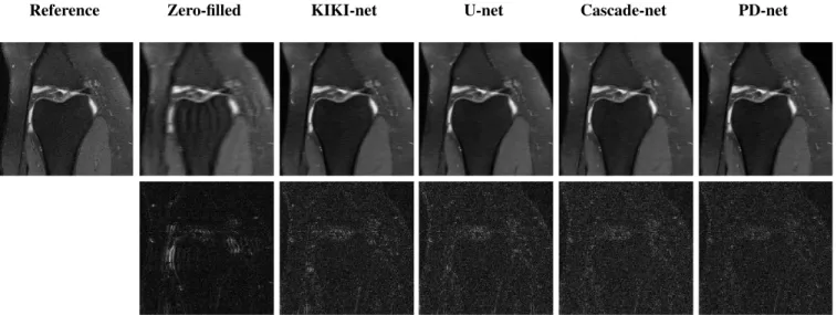
Fig. 2 shows the reconstruction obtained in the fastMRI for-mat (magnitude and cropped to 320 × 320 in the center) for a specific slice. We can see that the KIKI-net has a hard time reconstructing the finer structures and that the U-net creates some big unwanted artifacts. The residual of the PD-net is more evenly distributed on the image.

Reference Zero-filled KIKI-net U-net Cascade-net PD-net

Fig. 2. Reconstruction results for a specific slice (15th slice of file1000000, part of the validation set). The first row represents the reconstruction using the different methods, while the second represents the absolute error when compared to the reference.

4. DISCUSSION

The data used in this benchmark might be the primary reason as to why the results presented here are not as good as those presented in the original papers. Indeed, it presents several drawbacks, some of which can be adjusted in future studies or benchmarks. First, the k-spaces are zero-padded, so the nets are trying to predict a value in those points (when work-ing in the k-space), and will be penalized by the fact that they are “artificially” set to 0 (they are actually non-zero). Sec-ond, the data was seemingly acquired with an oversampled A/D. This results in a noise distribution with spatially varying variance, with an auto-correlation that could be mixed with the signal auto-correlation. A digital filtering step would be needed to obtain a white noise distribution. However, this reduces the matrix size, and the ground truth is not that of the original dataset anymore. Third, as knee has less signal than other organs, it might be more difficult to retrieve it and disentangle it from the noise. Fourth, the outer parts of the volumes in this dataset have almost no signal, therefore in-creasing the PSNR of the zero-filled reconstruction, even if it does not perform necessarily well in the signal-abundant re-gions of the volumes. Finally, as can be seen in the fastMRI challenge leaderboards2_{, parallel imaging will allow for}

bet-ter results, and it is important to also benchmark the gener-alizations of these approaches on this dataset (or generalize them if the generalization does not exist yet) in future work.

The networks used in this benchmark also present some aspects which can improved. Firstly, the duration of the train-ing is prohibitive as 300k steps of batch size 1, can last up

2_{https://fastmri.org/leaderboards}

to 2 days for the KIKI-net. This makes the iteration cycles very slow. Secondly, the justification behind using CNN in the k-space is not clear at all. Indeed, CNNs thrive when there is translation invariance, which is not the case in the k-space. The lower frequencies should definitely not be handled in the same way as the higher frequencies. Thirdly, Genera-tive Adversarial Networks (GANs) might help improve those networks by learning a part of the loss function. In the work introducing RefineGAN [7] for example, a GAN is used to improve the reconstruction of a U-net, but there is no funda-mental reason why GANs could not be added at the end of the other networks presented in this study. The work introducing DAGAN [17] does almost the same with the addition of an extra perceptual loss computed with a pre-trained VGG net-work [18]. Finally, the handling of complex values was not analyzed in this study. Indeed, the way the networks handle them is always by concatenating the real and imaginary parts, making the complex-valued image or the k-space a 2-channel real-valued image or k-space. Some other works, like the one introducing deep residual learning [19], use the phase and the magnitude of the complex numbers and take advantage of it in 2 separate ways.

5. ACKNOWLEDGEMENTS

We want to thank Jonas Adler, Justin Haldar and Jo Schlem-per for their very useful and benevolent remarks and answers they gave when asked questions about their works.

References

[1] J. Zbontar et al. fastMRI: An Open Dataset and Bench-marks for Accelerated MRI. Tech. rep.

[2] J. Cheng et al. Model Learning: Primal Dual Networks for Fast MR imaging. Tech. rep.

[3] T. Eo et al. “KIKI-net: cross-domain convolutional neural networks for reconstructing undersampled mag-netic resonance images”. In: Magmag-netic Resonance in Medicine80.5 (2018), pp. 2188–2201.

[4] J. Schlemper et al. “A Deep Cascade of Convolutional Neural Networks for MR Image Reconstruction”. In: IEEE Transactions on Medical Imaging 37.2 (2018), pp. 491–503.

[5] F. Chollet et al. Keras. https://keras.io. 2015. [6] A. Paszke et al. “Automatic differentiation in

Py-Torch”. In: (2017).

[7] T. Minh Quan, T. Nguyen-Duc, and W.-K. Jeong. Com-pressed Sensing MRI Reconstruction using a Genera-tive Adversarial Network with a Cyclic Loss. Tech. rep. [8] X. Glorot and Y. Bengio. “Understanding the difficulty of training deep feedforward neural networks”. In: Pro-ceedings of the thirteenth international conference on artificial intelligence and statistics. 2010, pp. 249–256. [9] O. Ronneberger, P. Fischer, and T. Brox. U-Net: Con-volutional Networks for Biomedical Image Segmenta-tion. Tech. rep.

[10] J. Adler and O. ¨Oktem. “Learned Primal-Dual Recon-struction”. In: IEEE Transactions on Medical Imaging 37.6 (2018), pp. 1322–1332.

[11] J. Caballero et al. “Dictionary learning and time sparsity for dynamic MR data reconstruction”. In: IEEE Transactions on Medical Imaging 33.4 (2014), pp. 979–994.

[12] A. L. Maas, A. Y. Hannun, and A. Y. Ng. “Rectifier nonlinearities improve neural network acoustic mod-els”. In: Proc. icml. Vol. 30. 1. 2013, p. 3.

[13] A. Chambolle and T. Pock. “A First-Order Primal-Dual Algorithm for Convex Problems with Applications to Imaging”. In: (2011), pp. 120–145.

[14] D. P. Kingma and J. Ba. Adam: A Method for Stochas-tic Optimization. 2014.

[15] R. Pascanu, T. Mikolov, and Y. Bengio. On the diffi-culty of training Recurrent Neural Networks. 2012. [16] S. Wang et al. “Accelerating magnetic resonance

imag-ing via deep learnimag-ing”. In: 2016 IEEE 13th Inter-national Symposium on Biomedical Imaging (ISBI). IEEE. 2016, pp. 514–517.

[17] P. L. Dragotti et al. “DAGAN: Deep De-Aliasing Gen-erative Adversarial Networks for Fast Compressed Sensing MRI Reconstruction”. In: IEEE Transactions on Medical Imaging37.6 (2017), pp. 1310–1321. [18] K. Simonyan and A. Zisserman. Very Deep

Convolu-tional Networks for Large-Scale Image Recognition. 2014.

[19] D. Lee et al. “Deep residual learning for accelerated MRI using magnitude and phase networks”. In: IEEE Transactions on Biomedical Engineering65.9 (2018), pp. 1985–1995.