HAL Id: inria-00072430
https://hal.inria.fr/inria-00072430
Submitted on 24 May 2006
HAL is a multi-disciplinary open access
archive for the deposit and dissemination of
sci-entific research documents, whether they are
pub-lished or not. The documents may come from
teaching and research institutions in France or
abroad, or from public or private research centers.
L’archive ouverte pluridisciplinaire HAL, est
destinée au dépôt et à la diffusion de documents
scientifiques de niveau recherche, publiés ou non,
émanant des établissements d’enseignement et de
recherche français ou étrangers, des laboratoires
publics ou privés.
Multiplication by an Integer Constant
Vincent Lefèvre
To cite this version:
Vincent Lefèvre. Multiplication by an Integer Constant. [Research Report] RR-4192, INRIA. 2001.
�inria-00072430�
ISRN INRIA/RR--4192--FR+ENG
a p p o r t
d e r e c h e r c h e
THÈME 2
Multiplication by an Integer Constant
Vincent Lefèvre
N° 4192
Vincent Lef`
evre
Th`eme 2 — G´enie logiciel et calcul symbolique
Projet SPACES
Rapport de recherche n 4192 — Mai 2001 — 17 pages
Abstract: We present and compare various algorithms, including a new one, allowing to perform multiplications by integer constants using elementary operations. Such algorithms are useful, as they occur in several problems, such as the Toom-Cook-like algorithms to mul-tiply large multiple-precision integers, the approximate computation of consecutive values of a polynomial, and the generation of integer multiplications by compilers.
Multiplication par une constante enti`
ere
R´esum´e : Nous pr´esentons et comparons divers algorithmes, dont un nouveau, permettant d’effectuer des multiplications par des constantes enti`eres `a l’aide d’op´erations ´el´ementaires. De tels algorithmes sont utiles, car ils interviennent dans plusieurs probl`emes, comme les algorithmes du style Toom-Cook pour multiplier des entiers `a grande pr´ecision, le calcul approch´e de valeurs cons´ecutives d’un polynˆome et la g´en´eration de multiplications enti`eres par les compilateurs.
1
Introduction
The multiplication by integer constants occurs in several problems, such as:
algorithms requiring some kind of matrix calculations, for instance the Toom-Cook-like algorithms to multiply large multiple-precision integers [7] (this is an extension of Karatsuba’s algorithm [3]),
the fast approximate computation of consecutive values of a polynomial [6] (we can use an extension of the finite difference method [4] that needs multiplications by constants), the generation of integer multiplications by compilers, where one of the arguments is statically known (some processors do not have an integer multiplication instruction, or this instruction is relatively slow).
We look for an algorithm that will generate code to perform a multiplication by an integer constant n, using left shifts (multiplications by powers of two), additions and subtractions. The other instructions available on processors, like right shifts, could be taken into account, but will not be used in the following.
We assume that the constant n may have several hundreds of bits. If it is large enough (several thousands of bits?), then fast multiplication algorithms of large integers can be used, without taking into account the fact that n is a constant.
To make the study of this problem easier, we need to choose a model that is both simple and close to the reality. We can assume that all the elementary operations (shifts by any number of bits, additions and subtractions) require the same computation time. This problem is much more difficult than the well-known addition chains problem [4]. A detailed formulation is given in Section 2.
The multiplication by an integer constant problem has already been studied for compilers, but for relatively small constants (on at most 32 or 64 bits). We do not know any algorithm that can generate optimal code in a reasonable time; thus we use heuristics.
A first (naive) heuristic will be described in Section 3.1. But most compilers implement an algorithm from Robert Bernstein [1] or a similar algorithm (taking into account the features of the target processor). In his article, Bernstein gives an implementation of his algorithm, but unfortunately with typos. Then Preston Briggs presented a corrected implementation in [2], but his code posted in 1992 to the comp.compilers1 newsgroup is also broken! This
implementation is shortly described in Section 3.2; I have rewritten it in order to perform some comparisons in Section 5.
The complexity (in time) of Bernstein’s algorithm is an exponential function of the constant size. It is fast enough for small constants, but much too slow for larger constants. For instance, even 64-bit constants may require more than one second on a 400 MHz G4 PowerPC, which may be too much for a compilation. I have found and implemented a completely different algorithm, that is fast enough for constants having several hundreds bits. It is presented in [5] and [6]. Section 3.3 gives a description and an improvement of
1
4 Vincent Lef`evre
this algorithm, which also allows to generate code to multiply a single number by several constants.
All these algorithms are compared in Section 5, both for the time complexity and the quality of the generated code.
2
Formulation of the Problem
A number x left-shifted k bit positions (i.e., x multiplied by 2k) is denoted x << k, and
the shift has a higher precedence than the addition and the subtraction (contrary to the precedence rules of some languages, like C or Perl). We assume that the computation time of a shift does not depend on the value k, called the shift count. Nowadays, this is true for many processors. Concerning the multiple precision, a shift consists of a shift at the processor level (where the shift count is bounded by the register size) and a shift by an integer number of words; thus, in the reality, a shift would be faster when k is an integer multiple of the register size. But it is difficult to take into account such considerations just now; we prefer to choose a simple model, that does not depend on the context.
In fact, in the algorithms we will describe, shifts will always be associated with an-other operation (addition or subtraction), and in practice, we will work with odd numbers only: shifts will always be delayed as much as possible. For instance, instead of performing x << 3 + y << 8, we will choose to perform (x + y << 5) << 3. This is a bit similar to floating-point operations, where a shift corresponds to an exponent change, but where shifts are actually performed only in additions and subtractions.
Thus the elementary operations will be additions and subtractions where one of the operands is left-shifted by a fixed number of bits (possibly zero, but this will never occur in the algorithms presented here), and these operations will take the same computation time, which will be chosen to be a time unit. Assuming that the operations x + y and x + y << k with k > 0 take the same computation time is debatable but reasonable. Indeed, with some processors (for instance, most ARM’s), such operations do take the same computation time (1 clock cycle). And we recall that in multiple precision, the computation time does not depend on the number of word shifts: the condition is not the fact that k is zero or not, but the fact that k is an integer multiple of the register size or not. Moreover, note that these assumptions modify the computation time by a bounded factor; as a consequence, a complexity of the form O(F (n)) is not affected by these assumptions.
Let n be a nonnegative odd integer (this is our constant). A finite sequence of nonnegative integers u0, u1, u2, . . . , uq is said to be acceptable for n if it satisfies the following properties:
initial value: u0= 1;
for all i > 0, ui= |siuj+ 2ciuk|, with j < i, k < i, si∈ {−1, 0, 1} and ci≥ 0;
final value: uq = n.
Thus, an arbitrary number x being given, the corresponding code iteratively computes uix from already computed values ujx and ukx, to finally obtain nx. Note that with this
formulation, we are allowed to reuse any already computed value. Therefore some generated codes may need to store temporary results. Moreover, the absolute value is only here to make the notations simpler and no absolute value is actually computed: if si = −1, we
always subtract the smaller term from the larger term.
The problem is to find an algorithm that takes the number n and that generates an acceptable sequence (ui)0≤i≤q that is as short as possible; q is called the quality (or length)
of the generated code (it is the average computation time when this code is executed under the condition that each instruction takes one time unit). But this problem is very difficult (comp.compilers contributors conjecture that it is NP-complete). Therefore we need to find heuristics.
Note: we restricted to nonnegative integers. We could have changed the formulation to accept negative integers (by removing the absolute value and letting the choice between uj
and uk to apply the sign si), but the problem would not be very different. We can also
extend the formulation to take into account even constants; then, we will allow a free left shift to be performed at the end (see the above paragraph on delayed shifts).
Also note that if ciand siare never zero (this will be the case in the considered heuristics),
then the ui are all odd.
3
Algorithms
3.1
The Binary Method
The simplest heuristic consists in writing the constant n in binary and generating a shift and an addition for each 1 in the binary expansion (taking the 1’s in any order): for instance, consider n = 113, that is, we want to compute 113x. In binary, 113 is written 11100012. If
the binary expansion is read from the left, the following operations will be generated: 3x ← x << 1 + x
7x ← 3x << 1 + x 113x ← 7x << 4 + x.
The number of elementary operations q is the number of 1’s in the binary expansion, minus 1. For random m-bit constants with uniform distribution, the average number of elementary operations, denoted qav, is asymptotically equivalent to m/2.
This method can be improved using Booth’s recoding, which consists in introducing signed digits (−1 denoted 1, 0 and 1) and performing the following transform as much as necessary: 0 1111 . . . 1111 | {z } k digits → 1 0000 . . . 000 | {z } k − 1 digits 1. This transform is based on the formula:
6 Vincent Lef`evre
This allows to reduce the number of nonzero digits from k to 2. As a digit 0 is transformed into a digit 1 on the left, it is more interesting to read the number from right to left: thus, the created 1 can be used in the possible next sequence of 1’s. For instance, 11011 would be first transformed into 11101, then into 100101. However, note that in general, there are several representatives having the same number of nonzero digits.
With the above example, 113 is written 100100012. Thus, Booth’s recoding allows to
generate 2 operations only, instead of 3:
7x ← x << 3 − x 113x ← 7x << 4 + x.
The number of elementary operations q is the number of nonzero digits (1 and 1), minus 1. And one can also prove that qav∼ m/3.
3.2
Bernstein’s Algorithm
Bernstein’s algorithm is based on arithmetic operations; it doesn’t explicitly use the binary expansion of n. It consists in restricting the operations to k = i − 1 and j = 0 or i − 1, si6= 0 and ci6= 0 in the formulation, and one of the advantages is that it can be used with
different costs for the different operations (the addition, the subtraction and the shifts). It is a branch-and-bound algorithm, using the following formulas:
Cost(1) = 0
Cost(n even) = Cost(n/2c odd) + ShiftCost
Cost(n odd) = min Cost(n + 1) + SubCost Cost(n − 1) + AddCost
Cost(n/(2c+ 1)) + ShiftCost + AddCost
Cost(n/(2c− 1)) + ShiftCost + SubCost
where the last two lines apply each time n/(2c+ 1) (resp. n/(2c− 1)) is an integer, c being
an integer greater or equal to 2.
Note that if n is odd, then n + 1 and n − 1 are even, therefore adding or subtracting 1 is always associated with a shift. As a consequence, assuming that the add and subtract costs are equal, we get back to our formulation.
The minimal cost and an associated sequence are searched for by exploring the tree. But there will be redundant searches. A first optimization consists in avoiding them with a memoization: results (for odd numbers only) are recorded in a hash table.
Sometimes, deep in a search, the cost associated with the partial path becomes greater than the current cost2; thus it is clear that this is a fruitless path, and it is useless to go
deeper: we prune the tree. Moreover, in order to avoid using fruitless paths too often, each time we come across a node, a lower bound of its cost is associated with it.
2
This cost is initialized with an upper bound, for instance by using the binary method, and it is updated each time a cheaper path is found.
The average time complexity seems to be exponential. The generated code cannot be longer than the one generated by the binary method, since the binary method corresponds to one of the paths in the search tree. But we do not know much more. Anyway, because of its complexity, this algorithm is too slow for large constants. This is why we will study new algorithms in the next section.
3.3
A Pattern-based Algorithm
3.3.1 A Simple Algorithm
This algorithm is based on the binary method: after Booth’s recoding, we regard the number n as a vector of signed digits 0, +1, −1, denoted respectively 0, P and N (and sometimes, 0, 1 and 1). The idea, that is recursively applied, is as follows: we look for repeating digit-patterns (where 0 is regarded as a blank), to make the most nonzero digits (P and N) disappear in one operation. To simplify, one only looks for patterns that repeat twice (though, in fact, they may repeat more often).
For instance, the number 20061, 1001110010111012 in binary, which is recoded to
P0P00N0P0N00N0P, contains the pattern P000000P0N twice: the first one in the positive form and the second one in the negative form N000000N0P. Thus, considering this pattern allows to make 3 nonzero digits (contrary to one with the binary method) disappear3in one
operation; thus we have reduced the problem to two similar (but simpler) problems: comput-ing the pattern P000000P0N and the remainder 00P000000000000. This can be summarized by the following double addition:
P000000P0N
- P000000P0N
+ 00P000000000000
---P0P00N0P0N00N0P
On this example, 4 operations are obtained (P000000P0N, 515 in decimal, is computed with 2 operations thanks to the binary method),
129x ← x << 7 + x
515x ← 129x << 2 − x
15965x ← 515x << 5 − 515x 20061x ← x << 12 + 15965x
whereas Bernstein’s algorithm generates 5 operations, that is one more than our algorithm. Now, it is important to find a good repeating pattern quickly enough. Let us give some definitions. A pattern is a sequence of nonzero digits up to a shift (for instance, P0N00N and P0N00N0are the same pattern) and up to a sign: if we invert each nonzero digit, we obtain
3
8 Vincent Lef`evre
the pattern under its opposite form (for instance, P0N00N becomes N0P00P). The number of nonzero digits of a pattern is called the weight of the pattern; the weight will be denoted w. We look for a pattern having a maximal weight. To do this, we take into account the fact that, in general, there are much fewer nonzero digits than zero digits, in particular near the leaves of the recursion tree, because of the following relation: w(parent) = 2 w(child 1)+w(child 2), child 1 being the pattern; child 2 is called the remainder. The solution is to compute all the possible distances between two nonzero digits, in distinguishing between identical digits and opposite digits. This gives an upper bound on the pattern weight associated with each distance4. For instance, with P0P00N0P0N00N0P:
operation distance upper bound weight
uj− 22uk 2 (P-N / N-P) 3 2 uj− 25uk 5 (P-N / N-P) 3 3 uj+ 27uk 7 (P-P / N-N) 3 2
The distances are sorted according to the upper bounds, then they are tested one after the other until the maximal weight and a corresponding pattern are found.
The complexity of the whole algorithm is polynomial, in O(m3) in the worst case, where
m is the constant’s length. Indeed, there are at most m0− 1 pattern searches (i.e., recursive
calls), where m0 is the number of nonzero digits (m0 ≤ m), and each pattern search has a
complexity in O(m2). After testing the current implementation on random values, we have
found that the average complexity of this implementation seems to be in Θ(m2), or a close
function.
3.3.2 Possible Improvements
Our algorithm can still be improved. Here are a few ideas proposed in [6]:
We can look for subpatterns common to different branches of the recursion. For in-stance, let us consider P0N0N00P0N0N000P0N and the pattern P0N0N. P0N appears twice: in the pattern P0N0N and in the remainder P0N; as a consequence, it can be computed only once (under the condition that P0N0N is computed in the right way, by making P0N appear). A solution will be given in the next section.
When looking for a repeated pattern, we can often have the choice between several patterns having the same maximal weight. Instead of choosing only one pattern, we can consider several of them, try them one after the other, and keep the shortest generated code. Ideally, we would test all the maximal-weight patterns, but we have to make sure that the complexity of the algorithm does not become exponential.
4
Only an upper bound, as a same nonzero digit cannot be used in both occurrences of the pattern at the same time.
We can consider the following transformation, which does not change the weight: P0N ↔ 0PP (and N0P ↔ 0NN). For instance, 110101010012 is encoded to P0N0P0P0P00P
by default, which gives a maximal weight of 1, therefore 5 generated operations; but the equivalent code P00N0NN0P00P is better: with the pattern P00N00N of weight 3, only 3 operations are generated. The drawback is the possibly exponential number of equivalent codes. Therefore it is not conceivable to always take all of them into account. We need a method allowing to quickly find the best transformations. For instance, it can be interesting, under some conditions, to perform the transformation as long as the weight of the currently considered pattern is not satisfactory; note that the number of P0N and N0P (in a same constant5) cannot be greater than the doubled
weight of the currently considered pattern. Or, once the pattern has been found, we can try to perform the transformation in order to add nonzero digits to the pattern, and therefore to increase its weight.
Using operations other than additions, subtractions and left shifts could be interesting, in particular the logical or, which suits the handling of binary data. But we would first have to separate positive and negative digits.
3.3.3 A New Algorithm (Common Subpatterns)
The generalization of the algorithm presented previously to the common subpattern search can be done quite naturally. In fact, we need to find an algorithm generating code for multiplying a single number by several constants at the same time, which is moreover useful when multiplying by constant matrices, for instance.
The problem is now: a set of constants written in binary using signed digits 0, P and N being given, find a maximal-weight pattern that appears twice (either in a same constant or in two different constants). Note that if such a pattern appears more than twice, it can naturally be reused later (this was not the case of the first algorithm).
Instead of looking for a distance leading to a pattern in a binary expansion (positive integer), we look for a triple (i, j, d) where i and j are numbers identifying the two constants ni and nj (possibly the same, i.e., i = j) in the set, and d a distance (or shift count)6, with
the following restrictions for symmetry reasons: 1. i ≤ j;
2. if i = j, then d > 0.
Once the pattern, denoted np, of weight greater or equal to 2 has been found, we compute the
binary expansion of the new constants n0 iand n 0 j (n 0 ionly, if i = j) satisfying ni= n0i± 2 cn p
and nj = n0j± 2c−dnp for some integer c (or ni = n0i± 2cnp± 2c−dnp if i = j)7, then we
5
We have to be precise on this point, in the case we would want to apply these transformations in the algorithm described in Section 3.3.3; however, for this algorithm, we will consider pairs of constants and this will not change much.
6
For instance, this is the difference between the exponents of the rightmost digit of the pattern occur-rences.
7±
10 Vincent Lef`evre
remove ni and nj from the set, then add n0i, n 0
j and np to the set (with the exception that
0 and 1 are never added to the set, because they cannot yield a pattern). We reiterate until there are no more patterns of weight greater or equal to 2; we use the binary method for the remaining constants. We do not want to discuss the implementation details in this paper; they are left to the reader.
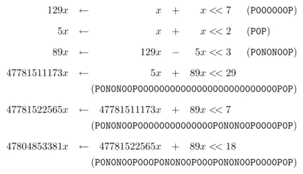
Now, let us illustrate this algorithm more precisely with an example: 47804853381, which is written 1011001000010110010000101100100001012 in binary, and after Booth’s
recoding: P0N0N00P000P0N0N00P000P0N0N00P0000P0P. As there is only one constant for the time being, the first step is similar to the one of the previous algorithm. We find the triple8 (0, 0, 11), the corresponding pattern is P0N0N00P, and the remainder is
P0N0N00P00000000000000000000000000P0P(there would be other choices). The set is now: { P0N0N00P00000000000000000000000000P0P, P0N0N00P }.
We find the triple (0, 1, 29), the corresponding pattern is P0N0N00P (i.e., still the same one), and the remainder is P0P. The set is now:
{ P0P, P0N0N00P }.
We find the triple (0, 1, −3), the corresponding pattern is P0P, and the remainder is P000000P. The set is now:
{ P000000P, P0P }.
Now, we cannot find any longer a repeating pattern whose weight is greater or equal to 2. Therefore we use the binary method for the remaining constants.
The generated code (6 operations) is given in Table 1.
Concerning the complexity, while the number of possible distances was in O(m) for the previous algorithm, the number of possible triples is here in O(m2). This tends to increase
the complexity, both in time and in space. However, by testing the current implementation on random values, we have found that the average time complexity of this implementation seems to be in Θ(m2), or a close function.
4
Searching for Costs With a Computation Tree
We are interested in the search for optimal costs. We can use properties of the optimal cost function qopt, coming from algebraic properties of the multiplication. Thus we will define a
function f having values in N (nonnegative integers) and bounding above qopt.
First, since we are interested in the optimal cost, we have to take into account the fact that even numbers can be generated by an optimal algorithm, due to a zero-bit shift (ci= 0
in the formulation). To avoid obtaining a function partly defined on even numbers, we want to define the function f on N∗(positive integers), in such a way that for all n ∈ N∗, we have:
8
Constants are numbered starting from 0. As there is one constant at this iteration, then i = j = 0.
129x ← x + x << 7 (P000000P) 5x ← x + x << 2 (P0P) 89x ← 129x − 5x << 3 (P0N0N00P) 47781511173x ← 5x + 89x << 29 (P0N0N00P00000000000000000000000000P0P) 47781522565x ← 47781511173x + 89x << 7 (P0N0N00P00000000000000P0N0N00P0000P0P) 47804853381x ← 47781522565x + 89x << 18 (P0N0N00P000P0N0N00P000P0N0N00P0000P0P)
Table 1: Code generated by the common-subpattern algorithm to compute 47804853381x. f (2n) ≤ f (n). Note that the possible additional shift is regarded as “delayed”, as this has been explained in Section 2, therefore it does not generate an additional cost.
Thus the function f is the greatest function from N∗to N taking the value 0 in 1 and in
2, and satisfying the following two properties (which are also properties of the optimal cost function qopt):
Let a and b be positive integers. Without loss of generality, we can assume that a > b. Then f (a ± b) ≤ f (a) + f (b) + 1. This property can be seen as a conse-quence of the distributivity of the addition and the subtraction over the multiplication: (a ± b)x = ax ± bx.
Let a and b be positive integers. Then f (ab) ≤ f (a) + f (b). This property can be seen as a consequence of the associativity of the multiplication: (ab)x = a(bx).
Note: the cost function for the addition and subtraction chains problem satisfies the same properties. The only difference is that we have here: f (2) = 0.
To compute this function, we can start by determining the inverse images of 0 (these are the powers of 2), then successively the inverse images of i = 1, 2, 3, and so on, using the first property with a and b such that f (a) + f (b) = i − 1 and the second property with a and b such that f (a) + f (b) = i. The only problem is that the considered sets are infinite; in practice, we choose to limit to a fixed interval J1, nK and we find a function fn satisfying
fn≥ f ≥ qopt.
Note that directly from the formulation of the problem, the computations can be rep-resented as a DAG (directed acyclic graph), the cost being the number of internal nodes
12 Vincent Lef`evre
(which represent shift-and-add operations). If we wish to compute the cost function for ev-ery integer (like what we are doing here) by memorizing only the values of this function, we can no longer take into account the reuse of the intermediate results, and we obtain a tree instead of a DAG. Here, we also have a tree, but a node can also represent a multiplication to take into account some forms of the reuse of results; such a node does not enter into the final cost. For instance, 861 = 21×41 can be computed from 21 = 101012and 41 = 1010012:
861 has a multiply node (cost 0) with parents 21 (cost 2) and 41 (cost 2), which gives a total cost of 4; 41 is used 3 times (861 = 41 << 4 + 41 << 2 + 41), but its cost has been counted only once in the total cost.
5
Results and Comparison of the Algorithms
We will not give any execution time of the algorithms, since contrary to Bernstein’s algo-rithm, which has been implemented in C and carefully optimized, the algorithms based on pattern searching are still in an experimental stage: they are implemented in Perl, using high-level functions for more readability and easier code maintenance, and are not optimized at all.
Table 2 gives, for each value of q up to 9, the smallest values for which the algorithm using common subpatterns (described in Section 3.3.3) generates a code whose length is greater or equal to q. Note that the value corresponding to q = 4 could be computed with 3 operations by avoiding Booth’s recoding and considering the pattern 101. Similarly, the value corresponding to q = 5 could be computed with 4 operations only by considering 11010101001 (instead of 101010101001) and the pattern 101.
q m smallest value 1 2 3 11 2 4 11 1011 3 6 43 101011 4 8 213 11010101 5 11 1703 11010100111 6 14 13623 11010100110111 7 18 174903 101010101100110111 8 21 1420471 101011010110010110111 9 24 13479381 110011011010110111010101
Table 2: For each value of q up to 9, the smallest values for which the algorithm using common subpatterns generates a code whose length is greater or equal to q.
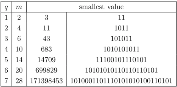
By way of comparison, Table 3 gives, for each value of q up to 7, lower bounds on the smallest value for which one obtains a code whose length is greater or equal to q with an optimal algorithm. These results have been obtained by an exhaustive search up to a given value; it is conjectured that they are exactly the smallest values (perhaps except for q = 7). Results for q = 6 and q = 7 were found by Ross Donelly, who performed a search up to one billion and posted the results to the rec.puzzles newsgroup. I found the same result for q = 6 (using a different code).
q m smallest value 1 2 3 11 2 4 11 1011 3 6 43 101011 4 10 683 1010101011 5 14 14709 11100101110101 6 20 699829 10101010110110110101 7 28 171398453 1010001101110101010100110101
Table 3: For each value of q up to 7, lower bounds on the smallest value for which one obtains a code whose length is greater or equal to q with an optimal algorithm; in fact, it is conjectured that these are exactly the smallest values (perhaps except for q = 7).
The highest difference in the code quality between Bernstein’s algorithm and our algo-rithm for numbers between 1 and 220is obtained for n = 543413; our algorithm generates 4
operations:
1. 255x ← x << 8 − x
2. 3825x ← 255x << 4 − 255x 3. 19125x ← 3825x << 2 + 3825x 4. 543413x ← x << 19 + 19125x whereas Bernstein’s algorithm generates 8 operations:
1. 9x ← x << 3 + x 2. 71x ← 9x << 3 − x 3. 283x ← 71x << 2 − x 4. 1415x ← 283x << 2 + 283x 5. 11321x ← 1415x << 3 + x 6. 33963x ← 11321x << 2 − 11321x 7. 135853x ← 33963x << 2 + x 8. 543413x ← 135853x << 2 + x.
14 Vincent Lef`evre
However, Bernstein’s algorithm is also better than our algorithm on some constants; the highest difference can be up to 3 operations for numbers between 1 and 220.
Table 4 gives the average number of operations for an m-bit constant (2 ≤ m ≤ 27) with Bernstein’s algorithm,
our algorithm using common subpatterns (CSP),
the same algorithm but considering all the possible transformations P0N ↔ 0PP and N0P ↔ 0NN (CSP+),
a search for the costs using a computation tree (see Section 4),
an exhaustive search (on all possible DAG’s whose nodes represent additions or sub-tractions), by considering values up to one billion; as we performed a bounded search, the given results are only (good) approximations to the optimal values.
Note that our algorithm becomes better than Bernstein’s algorithm in average from m = 12 (which is more important, since we can use a table or a specific algorithm for small constants). The other two algorithms cannot be used as they are in the general case, but we can deduce the following points from the results:
it is a priori interesting to consider the transformations P0N ↔ 0PP and N0P ↔ 0NN (refer to the discussion in Section 3.3.2);
the search using a computation tree, which is based on an exhaustive search without trying to reuse intermediate results, seems to be better than the algorithms based on the search for common subpatterns, which, on the contrary, try to reuse intermediate results.
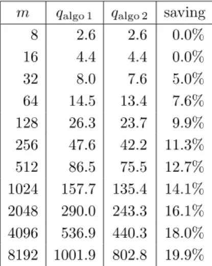
For much larger values of m, there are too many numbers to test; therefore we can only perform tests on random values. Moreover, Bernstein’s algorithm would take too much time. So, we decided to test only the algorithms based on pattern searching: the one described in Section 3.3.1 and the one described in Section 3.3.3. The results are given in Table 5.
It seems that in both above cases, we have qav= O(m/ log m), but the first values of qav,
though accurate, are not very significant to have an idea about the asymptotic behavior of qav, the next values are not very accurate and finally, we have few values in total. We need
to carry on with the computation of qav to have a better idea of its asymptotic behavior
(unless we can find a direct proof).
6
Conclusion
We described a new algorithm allowing to perform multiplications by integer constants. This algorithm can also be used to multiply a single number by different constants at the same time. But many questions have not been studied yet and remain open. In particular:
m Bernstein CSP CSP+ Tree DAG’s 2 1 ( 0.0 %) 1 ( 0.0 %) 1 ( 0.0 %) 1 (0.0 %) 1 3 1 ( 0.0 %) 1 ( 0.0 %) 1 ( 0.0 %) 1 (0.0 %) 1 4 1.5 ( 0.0 %) 1.5 ( 0.0 %) 1.5 ( 0.0 %) 1.5 (0.0 %) 1.5 5 1.75 ( 0.0 %) 1.75 ( 0.0 %) 1.75 ( 0.0 %) 1.75 (0.0 %) 1.75 6 2 ( 0.0 %) 2 ( 0.0 %) 2 ( 0.0 %) 2 (0.0 %) 2 7 2.281 ( 0.0 %) 2.313 ( 1.4 %) 2.281 ( 0.0 %) 2.281 (0.0 %) 2.281 8 2.563 ( 0.6 %) 2.578 ( 1.2 %) 2.547 ( 0.0 %) 2.547 (0.0 %) 2.547 9 2.758 ( 1.1 %) 2.836 ( 4.0 %) 2.75 ( 0.9 %) 2.727 (0.0 %) 2.727 10 3.047 ( 5.5 %) 3.066 ( 6.2 %) 2.945 ( 2.0 %) 2.887 (0.0 %) 2.887 11 3.287 ( 6.2 %) 3.311 ( 6.9 %) 3.176 ( 2.6 %) 3.096 (0.0 %) 3.096 12 3.534 ( 5.7 %) 3.532 ( 5.7 %) 3.406 ( 1.9 %) 3.343 (0.0 %) 3.343 13 3.765 ( 6.0 %) 3.762 ( 5.9 %) 3.621 ( 1.9 %) 3.554 (0.0 %) 3.553 14 4.009 ( 8.1 %) 3.985 ( 7.4 %) 3.818 ( 2.9 %) 3.724 (0.4 %) 3.710 15 4.246 (10.9 %) 4.204 ( 9.8 %) 4.011 ( 4.8 %) 3.876 (1.3 %) 3.828 16 4.479 (13.0 %) 4.422 (11.5 %) 4.209 ( 6.2 %) 4.071 (2.7 %) 3.964 17 4.712 (14.1 %) 4.639 (12.3 %) 4.405 ( 6.6 %) 4.269 (3.3 %) 4.131 18 4.944 (14.2 %) 4.848 (12.0 %) 4.588 ( 6.0 %) 4.461 (3.1 %) 4.329 19 5.174 (14.6 %) 5.060 (12.1 %) 4.769 ( 5.6 %) 4.624 (2.4 %) 4.514 20 5.403 (15.8 %) 5.268 (12.9 %) 4.953 ( 6.1 %) 4.765 (2.1 %) 4.667 21 5.630 (17.8 %) 5.475 (14.5 %) 5.132 ( 7.3 %) 4.904 (2.6 %) 4.780 22 5.858 (20.2 %) 5.677 (16.5 %) 5.312 ( 9.0 %) 5.071 (4.1 %) 4.871 23 6.083 (22.4 %) 5.880 (18.3 %) 5.487 (10.4 %) 5.252 (5.6 %) 4.972 24 6.309 (23.5 %) 6.078 (18.9 %) 5.657 (10.7 %) 5.433 (6.3 %) 5.110 25 6.532 (23.8 %) 6.277 (19.0 %) 5.827 (10.5 %) 5.589 (6.0 %) 5.274 26 6.755 (24.0 %) 6.473 (18.8 %) 5.999 (10.1 %) 5.721 (5.0 %) 5.447 27 6.978 (24.6 %) 6.668 (19.1 %) 6.170 (10.2 %) 5.841 (4.3 %) 5.599 Table 4: Average number of operations for a m-bit constant with Bernstein’s algorithm, with our algorithm using common subpatterns (CSP), with the same algorithm but considering all the possible transformations P0N ↔ 0PP and N0P ↔ 0NN (CSP+), with a search for the costs using a computation tree (note: these results are not proved, for we have taken the function fn with n = 229; however, there should not be any difference, with the given precision), and
with an exhaustive search up to one billion (conjectured optimal). The percentages represent the loss relative to the exhaustive search costs. Note: these means were computed by using all the m-bit constants.
16 Vincent Lef`evre
m qalgo 1 qalgo 2 saving
8 2.6 2.6 0.0% 16 4.4 4.4 0.0% 32 8.0 7.6 5.0% 64 14.5 13.4 7.6% 128 26.3 23.7 9.9% 256 47.6 42.2 11.3% 512 86.5 75.5 12.7% 1024 157.7 135.4 14.1% 2048 290.0 243.3 16.1% 4096 536.9 440.3 18.0% 8192 1001.9 802.8 19.9%
Table 5: Average number of operations for a m-bit constant with both algorithms based on pattern searching (described in Sections 3.3.1 and 3.3.3). These numbers were computed by considering random m-bit constants, therefore they are approximate numbers. The saving is the value of 1 − qalgo 2/qalgo 1.
Is this problem NP-complete? What can be said about the asymptotic behavior of the optimal quality (in average, in the worst case)? Same question concerning the various heuristics. What complexity (in average, in the worst case, in time, in space) can be obtained?
How can the heuristics be improved? Is it interesting to use other elementary opera-tions, like right shifts or the logical or ?
How much memory does the generated code take, that is, how many temporary results need to be saved? How can temporary results be avoided?
Other ways can be explored to find new heuristics. For instance, can we find interesting algorithms by writing the constant in a properly chosen numeration system?
The following relation on the positive integers can be defined: m n if the computa-tion of n can use m as a temporary result. The best would be to apply this definicomputa-tion to the set of the optimal computations9. Note that n n and that insofar as the
cost of an integer is well-defined (it is the quality of the generated code), one has m n ⇒ q(m) < q(n); as a consequence, the relation is antisymmetric. But it is not
9
It can also be applied to the codes generated by a particular heuristic, but this would not necessarily be interesting.
necessarily transitive. The study of this relation, for instance knowing the numbers that have many “successors”, could allow to find other heuristics.
7
Thanks
The results given in the tables of Section 5 required heavy computations; most of these computations have been performed on machines from the MEDICIS10computation center,
I wish to thank. I would also like to thank Ross Donelly for his results.
References
[1] R. Bernstein. Multiplication by integer constants. Software – Practice and Experience, 16(7):641–652, July 1986.
[2] P. Briggs and T. Harvey. Multiplication by integer constants. ftp://ftp.cs.rice.edu/public/preston/optimizer/multiply.ps.gz, July 1994.
[3] A. Karatsuba and Y. Ofman. Multiplication of multidigit numbers on automata. Soviet Phys. Doklady, 7(7):595–596, January 1963.
[4] D. Knuth. The Art of Computer Programming, volume 2. Addison Wesley, 1973. [5] V. Lef`evre. Multiplication by an integer constant. Research report RR1999-06,
Labora-toire de l’Informatique du Parall´elisme, Lyon, France, 1999.
[6] V. Lef`evre. Moyens arithm´etiques pour un calcul fiable. PhD thesis, ´Ecole Normale Sup´erieure de Lyon, Lyon, France, January 2000.
[7] D. Zuras. More on squaring and multiplying large integers. IEEE Transactions on Computers, 43(8):899–908, August 1994.
10
Unité de recherche INRIA Lorraine
LORIA, Technopôle de Nancy-Brabois - Campus scientifique
615, rue du Jardin Botanique - BP 101 - 54602 Villers-lès-Nancy Cedex (France)
Unité de recherche INRIA Rennes : IRISA, Campus universitaire de Beaulieu - 35042 Rennes Cedex (France) Unité de recherche INRIA Rhône-Alpes : 655, avenue de l’Europe - 38330 Montbonnot-St-Martin (France) Unité de recherche INRIA Rocquencourt : Domaine de Voluceau - Rocquencourt - BP 105 - 78153 Le Chesnay Cedex (France)
Unité de recherche INRIA Sophia Antipolis : 2004, route des Lucioles - BP 93 - 06902 Sophia Antipolis Cedex (France)
Éditeur
INRIA - Domaine de Voluceau - Rocquencourt, BP 105 - 78153 Le Chesnay Cedex (France)
http://www.inria.fr ISSN 0249-6399