Analysis of soil penetrometer using Eulerian finite element method

ANALYSIS OF SOIL PENETROMETER USING

EULERIAN FINITE ELEMENT METHOD

BY

SHUANG HU

B.S. IN HYDRAULIC ENGINEERING (1998)

TSINGHUA UNIVERSITY

MASTER OF PHILOSOPHY IN CIVIL ENGINEERING (2000)

HONG KONG UNIVERSITY OF SCIENCE AND TECHNOLOGY

SUBMITTED TO THE DEPARTMENT OF CIVIL AND ENVIRONMENTAL ENGINEERING IN PARTIAL FULFILLMENT OF THE REQUIREMENTS FOR

THE DEGREEE OF

MASTER OF SCIENCE IN CIVIL AND ENVIRONMENTAL ENGINEERING

AT THE

MASSACHUSETTS INSTITUTE OF TECHNOLOGY JUNE 2003

© 2003 Massachusetts Institute of Technology. All rights reserved.

Signature of Author:

Departme>9fvil and-Epvirorknental Engineering, May 9, 2002 Certified by:

rofessor And/ J. Whittle, Thesis Supervisor

Accepted by:

Professor Oral Buyukozturk, Chairman, Departmental Committee on Graduate Students

MASSACHUSETTS INSTITUTE OF TECHNOLOGY

BARKER

JUN 0 2 2003

ANALYSIS OF SOIL PENETROMETER USING

EULERIAN FINITE ELEMENT METHOD

BY

SHUANG HU

Submitted to the Department of Civil and Environmental Engineering

on May 9, 2003 in Partial Fulfillment of the

Requirements for the Degree of Master of Science in Civil and Environmental Engineering

ABSTRACT

This thesis investigates the use of an Eulerian Finite Element (EFE) method for modeling penetration in soils. The formulation decouples material and nodal points displacements such that soil flows through a fixed finite element mesh. This approach eliminates problems of mesh distortion associated with conventional Lagrangian formulations but requires special procedures to convect the soil constitutive law and prevent numerical diffusion. The current analyses use the program DiekA, developed at the University of Twente in the Netherlands. Detailed calculations have been performed to investigate the effects of elements size and load/time step size on the stability and accuracy of the numerical simulations. Computed results for undrained penetration in homogeneous clays are similar to prior predictions from approximate steady state formulations such as the Strain Path Method. Further calculations for two-layer systems illustrate the potential of the Eulerian formulation to handle realistic layered soil profiles. A more limited study confirms the complexity of drained penetration in sands, where the predicted tip resistance is affected by soil friction and dilation angles, in situ stresses, and moduli. Further study is needed to establish the role of interface friction and lateral earth pressure. The results in the thesis present a first step towards implementation of more advanced effective stress

soil models in EFE analyses of penetration in layered soils.

ACKNOWLEDGMENTS

I wish to express my sincere thanks to all those who helped to bring about the

completion of this research program.

Firstly, special thanks are due to my supervisor, Prof. Andrew Whittle, who introduced this topic to me and provided constant guidance all the way. He provided invaluable feedback and assistance during the course of this research. His advice and comments made during the preparation of this thesis were also very much valued and greatly appreciated.

I would like to express my great appreciation to Gert-Jan Schotmeyer from

GeoDelft and Ton van den Boogaard from University of Twente, for giving me constant and patient help on DiekA coding. Thanks for putting up with my long emails full of questions.

Also, I want to thank my "soil and rock" friends on the third floor of Buildingl, and friends from other departments. Thanks for the fun we had together, the nice food you made for me, the happiness we shared, and a sympathetic ear when

I feel frustrated.

Finally, but most importantly, I wish to thank my family for their endless love and support. Particularly, I want to say 10 thanks to my husband, Shangwen Wei, for his constant encouragement, looking after me, sharing both my sorrows and joys all the way, and for the love I treasure forever.

TABLE OF CONTENTS

ABSTRACT... 2

ACK NO W LEDG M ENTS ... 3

TABLE O F CONTENTS... 4

LIST O F FIGURES... 7

LIST O F TABLES ... 12

CH APTER 1 INTRO DUCTION ... 13

1.1 PROBLEM STATEMENT AND SCOPE OF STUDY ... 13

1.2 ORGANIZATION OF THESIS... 15

CH APTER 2 LITERATURE REVIEW ... 16

2.1 BEARING CAPACITY THEORY ... 16

2.2 CAVITY EXPANSION THEORY ... 19

2.3 STEADY STATE FLOW ... 24

2.4 INCREMENTAL FINITE ELEMENT M ETHOD... 26

CHAPTER 3 EULERIAN FORMULATION FOR FINITE ELEMENT ANALYSIS OF PENETRATIO N PRO BELM S...39

3.1 BASIC EQUATIONS...39

3.2 CONVECTION ITEM ... 45

3.3 LAYERED DEPOSITS WITH EULERIAN APPROACH ... 49

4.2 NUMERICAL ACCURACY AND INTERPRETATION OF PENETRATION SIMULATION ... 55

4.2.1 Numerical Accuracy... 55

4.2.2 Interpretation of Penetration Simulation ... 56

4.3 EFFECT OF SOIL STIFFNESS... 60

4.4 LAYERED CLAY ... ...-61

CHAPTER 5 PENETRATION ANALYSIS IN SAND ... 84

5.1 DRAINED SHEAR STRENGTH OF SANDS ... 84

5.2 FRICTION ANGLE ...-- 89

5.3 NUMERICAL SIMULATION... 89

5.4 EFFECT OF STRENGTH PARAMETERS ... 93

CHAPTER 6 IMPLEMENTATION OF USER MATERIAL MODEL INTO DIEKA...117

6.1 INTRODUCTION ... 117

6.2 THREE ROUTINES FOR USER SUPPLIED M ATERIAL M ODEL ... 117

6.2.1 User Supplied Initial Routine...118

6.2.2 User Supplied Stress Update Routine ... 119

6.2.3 User Supplied M atrix Routine... 121

6.3 VALIDATION OF USER SUPPLIED MATERIAL M ODEL ... 123

6.4 INITIALIZATION OF STATE VARIABLES ... 124

CHAPTER 7 SUMMARY, CONCLUSIONS AND SUGGESTIONS FOR FUTURE STUDIES 127 7.1 SUMMARY AND CONCLUSIONS...127

7.2 SUGGESTIONS FOR FUTURE STUDIES ... 129

7.2.1 M odel interface friction...129

7.2.3 Implementing advanced soil models into DiekA ... 129

APPENDIX A AN INPUT FILE FOR DIEKA ... 130

APPENDIX B USER PROVIDED SUBROUTINES FOR A LINEARLY ELASTIC AND PERFECTLY PLASTIC M ATERIAL M ODEL... ... .... ---... 155

B.] Initialization routine USRINI...155

B.2 Stress Update Routine USRSIG...157

B.3 Stiffness Update Routine USRM TX...157

LIST OF FIGURES

Figure 2.1 Assumed failure mechanisms under deep foundations (Durgunoglu

and M itchell, 1975)... 29

Figure 2.2 Assumed relationship between cone resistance and cavity limit p ressure ... . . 30

Figure 2.3 Relation between Nq and

#peak

Figure 2.4 Comparison of N, from different methods... 31

Figure 2.5 Predicted deformation pattern around simple pile (Baligh, 1975)... 32

Figure 2.6 Predicted deformation pattern around a 60-degree cone (Levadoux, 19 8 0 )... . . 33

Figure 2.7 Predicted deformation pattern around a FMMG piezoprobe (Sutabutr, 199 9)... . . 34

Figure 2.8 Steady state behavior (Yu et al., 2000)... 35

Figure 2.9(a) Typical contour plot for strain y (Yu et al., 2000)... 36

Figure 2.9(b) Contour plot for strain y during simple pile penetration (Baligh, 19 8 5)... . . 3 6 Figure 2.10(a) Typical contour plot for excess pore pressure (Yu et al., 2000).. 37

Figure 2.10(b) Excess pore pressure due to undrained simple pile penetration (B aligh , 1985)... 37

Figure 3.1 Node and material point displacement at one step ... 52

Figure 3.2 Definitions for moving material boundary through fixed FE mesh (V an den B erg, 1996)... 52

Figure 4.1 Piezocone tip geom etry... 66

Figure 4.2 Finite element mesh for penetration analysis... 66

Figure 4.3 Rounded cone-cylindar transition part... 67

Figure 4.4 504 elements and 5184 elements FE mesh ... 68

Figure 4.5 Pressure-displacement curves for 504, 1944 and 5184 elements ... 69

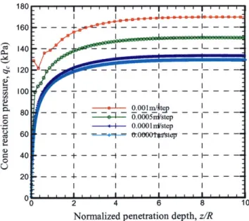
Figure 4.6 Pressure-displacement curves for varying step sizes... 69

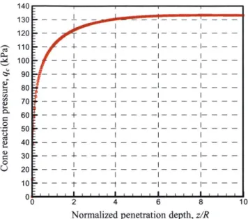
Figure 4.7 Pressure-displacement curve for basic calculation ... 70

Figure 4.8(a) Contours of equivalent plastic strain Ep ... 71

Figure 4.8(b) Equivalent plastic strain Ep along the penetrometer shaft... 71

Figure 4.9(a) Octahedral stress increment Au.e, /o . . ..... . . .. . . .. . . . 72

Figure 4.9(b) Au ,,,, /o , along shaft ... 72

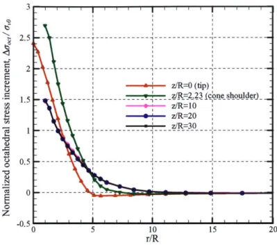
Figure 4.9(c) Radial distribution of Ac,,, /o e at various elevations... 73

Figure 4.10(a) Contours of shear stress ,, I/o 0 .... . . . . . . 74

Figure 4.10(b) z,, /a,0 along the penetrometer shaft... 74

Figure 4.11 Contours of vertical stress ,

/.

Figure 4.12 Contours of radial stress a,/o o ... 75

Figure 4.13 Contours of circumferential stress o,, /o . . . 76

Figure 4.14 O-,z /oV o ,, /0vo , o700

/oro

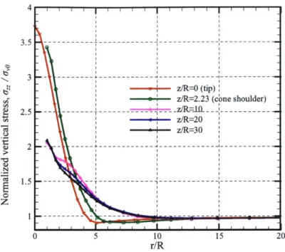
Figure 4.15 Radial distribution of o /o-0, at various elevations ... 77

Figure 4.16 Radial distribution of o-, /o 0e at various elevations ... 77

Figure 4.18(a) Contours of normalized cylindrical expansion shear stress qh /UvO

... 7 9

Figure 4.18(b) qhl/ v0 along shaft ... . 79

Figure 4.18(c) Radial distribution of qh /v0 at various elevations ... 80

Figure 4.19 Pressure-displacement curves for clays with different Ir... 81

Figure 4.20 Cone factor comparison of analyszed results with published so lu tio n s ... 8 1 Figure 4.21 Layered clay - location of initial layer boundary ... 82

Figure 4.22 Pressure-displacement curve for penetration in layered clay ... 82

Figure 4.23 Pressure-displacement curves for layered system with different Ir ra tio ... 8 3 Figure 5.1 Mohr-Coulomb model ... 98

Figure 5.2 Drucker-Prager m odel... 98

Figure 5.3 Matching Mohr-Coulomb model and Drucker-Prager model ... 99

Figure 5.5 Pressure-displacement curves for Drucker-Prager and Mohr-Coulomb m odels, base case analysis ... 100

Figure 5.6(a) Contours of mobilized friction angle - Mohr-Coulomb criterion 101 Figure 5.6(b) Contours of mobilized friction angle - Drucker-Prager criterion 101 Figure 5.7(a) Contours of equivalent plastic strain E ... 102

Figure 5.7(b) Equivalent plastic strain Ep along the penetrometer shaft... 102

Figure 5.7(c) Radial distribution of Ep at various elevations... 103

Figure 5.8(a) Octahedral stress increment A ', /o- ... ... 104

Figure 5.8(c) Radial distribution of Ac', /0o at various elevations... 105

Figure 5.9(a) Contours of shear stress ,

/

Figure 5.9(b) r, /o along the penetrometer shaft... 106

Figure 5.9(c) Radial distribution of z,,

/a',

Figure 5.10 Contours of vertical stress o /a ... 108

Figure 5.11 Contours of radial stress o'

/o

Figure 5.12 Contours of circumferential stress o'

/

Figure 5.13 o'

/

/a'o,

Figure 5.14 Radial distribution of a'

/'

Figure 5.15 Radial distribution of a' /0'0 at various elevations ... 110

Figure 5.16 Radial distribution of o' /o-' at various elevations... 111

Figure 5.17(a) Contours of normalized cylindrical expansion shear stress qh /O ... 1 12 Figure 5.17(b) qh / o along shaft ... 112

Figure 5.17(c) Radial distribution of q

/ro

Figure 5.18 Correlation between cone factor Nq and friction angle

#

Figure 5.19 Pressure-displacement curves for varying

#

Figure 5.20 Pressure-displacement curves for varying V (# = 45

)...

Figure 5.21 Pressure-displacement curves for varying stiffness E ... 116

Figure 6.1 Fitting Tresca and von Mises models at triaxial compression mode 126 Figure 6.2 Load-displacement curves for different material models ... 126

Figure A. 1 Input file example "init.inv"... 139

Figure A.2 Finite element mesh represented by the example input file... 140

Figure A.3 Rounded cone-cylindar transition part... 140

Figure A.4 Output file "vorm.dat" for "init.inv"... 154

Figure B. 1 "USRINI" file for linearly elastic and perfectly plastic model with von M ises yielding ... 159

Figure B.2 Statements in input file for user defined material... 160

Figure B.3 "USRSIG" file for linearly elastic and perfectly plastic model with von M ises yielding ... 165

Figure B.4 Flow chart of incremental algorithm for linearly elastic and perfectly plastic model with von Mises yielding... 166

Figure B.5 "USRMTX" file for linearly elastic and perfectly plastic model with von M ises yielding ... 170

LIST OF TABLES

Table 4.1 Material parameters for clays with varying rigidity index... 64 Table 4.2 Material parameters for clays with varying u,0... . . . .. . . .. . . 64

Table 4.3 Material parameters and initial stress for penetration analysis in layered clays... 65

Table 5.1 Material data used in sensitivity analysis... 96

CHAPTER 1

INTRODUCTION

1.1

Problem Statement and Scope of Study

Soil penetration is involved in many practical geotechnical problems, for example,

foundation elements (piles, caissons, etc.), in situ testing devices (piezocone,

dilatometer, etc.), the continuous soil-sampling test, vane test and more. The analysis

of the cone resistance, the evolution of stresses and strains produced in the soil during

the penetration process, are all of relevant interest in geotechnical engineering.

This research focuses on the process of piezocone penetration. The piezocone

penetration testing (PCPT) has become a useful tool for in situ investigation and

geotechnical design. Geotechnical engineers have found that the continuous sounding

cone penetration provides excellent resolution of vertical stratigraphy in soil

exploration projects (e.g. Lunne, et al., 1997). The use of PCPT data for estimating

soil properties requires reliable correlations between PCPT testing results (cone

resistance, sleeve friction ratio and pore pressures measured both during steady

penetration and in subsequent consolidation) and soil engineering properties.

As pointed out by Baligh (1985), the penetration in the soil is particularly

difficult in terms of theoretical analysis, due to the following features: (1) singularities

and high gradients of the field variables (displacements, stresses, strains and pore

water pressures) around the penetrometer; (2) large deformations and strains

non-linearity, anisotropy, time-dependency and frictional response; (4) drainage conditions (controlled by consolidation characteristics of the soil); and (5) non-linear penetrometer-soil interface characteristics.

Due to the complex geometry of the penetration problem, analytical tools can normally only be used in an approximate manner. Nevertheless, many analytical solutions have been developed in geotechnical practice, for example, bearing capacity (Meyerhof, 1961), and cavity expansion theories (Vesic, 1972). Bearing capacity solutions assume rigid, perfectly plastic soil behavior and are generally solved by limit equilibrium methods (Vesic, 1977). Cavity expansion theory assumes one-dimensional deformation/strain field and most solutions consider elastic, perfectly plastic material response with Tresca or Mohr-Coulomb yield criteria (Yu, 2000). Some cavity expansion solutions are developed with Modified Cam Clay model (Yu

et al., 2000)

In principal, numerical techniques, in particular the finite element method can allow a more complete solution of the penetration problem, by taking into account the penetrometer geometry, interface properties and soil constitutive behaviors. A large-strain finite element formulation is needed, to carry out the penetration analysis. The use of conventional Updated Lagrangian methods quickly results in highly distorted elements, yielding highly inaccurate answers or even divergence of the computational procedure. In order to address this problem, one option is to use remeshing techniques (e.g., Hu and Randolph, 1997). Alternatively Eulerian finite element formulations proposed by van den Berg (1994, 1996) consider the flow of soil around the penetrometers.

Van den Berg's method is followed in this research. A finite element program "DiekA", developed at University of Twente in Netherlands (DiekA development group, 2000), is applied for this study to investigate the use of DiekA in penetration analysis. Penetration analyses on clays and sands, homogeneous and layered soils, are performed. The detailed stress/strain fields from the FE analysis are explored for a clear interpretation of the penetration mechanism. A series parametric study is carried out in each case to evaluate the main factors affecting predictions of penetration tip resistance.

1.2

Organization Of Thesis

The thesis is organized as follows. Following a brief introduction in this chapter, Chapter 2 surveys existing methods for penetration analysis. Basic ideas behind each method are presented together with a comparison of their relative advantages and disadvantages. Chapter 3 summarizes the formulation of the Finite Element Program DiekA. Chapter 4 presents results of undrained penetration analyses in homogeneous clays and layered clay profiles. Chapter 5 explores drained penetration analyses for sands. In order to develop a more reliable basis for predicting penetration processes, advanced soil models need to be implemented into DiekA. Implementation of a user defined material model (linear elastic perfectly plastic model) into DiekA is demonstrated in Chapter 6. Finally, Chapter 7 presents a summary and conclusions from this work together with recommendations for future studies.

CHAPTER 2

LITERATURE REVIEW

There have been extensive research efforts to develop reliable correlations between

cone resistance and soil properties. For example, Sanglerat (1972) summarizes

correlations between cone resistance and relative density, deformation characteristics

of the soil, etc. Theoretical analyses of cone penetration can be classified into four

main categories: (1) Bearing capacity theories; (2) cavity expansion methods; (3)

steady state penetration models and (4) incremental finite element analyses. This

chapter presents the basic concepts underlying these approaches together with their

capabilities and limitations.

2.1

Bearing Capacity Theory

Bearing capacity theory is the earliest method used to analyze cone penetration. In

this approach, the cone penetration problem is considered as an incipient failure for a

rigid perfectly plastic soil. Solutions have been based on limit equilibrium (Meyerhof,

1961; Vesic, 1977) and slip-line methods analyses (Sokolovskii, 1965). Well-known

solutions are those published by Meyerhof (1961), Durgunoglu and Mitchell (1975).

Figure 2.1 shows some of the failure patterns that have been used to analyze deep

penetration problems (Durgunoglu and Mitchell, 1975). Bearing capacity theories

have been widely used in soil mechanics due to its simplicity. However, the solutions

from limit equilibrium methods are only approximate, because of the following

and (3) use of shape factor to convert from a planar wedge to axisymmetric cone

penetration introduces uncertainty. It should also be pointed out that the shear

surfaces shown in Figure 2.1 are not generally observed during deep cone penetration

process.

In slip-line method (Sokolovskii, 1965), a set of differential equations is given

by combining the equilibrium equations with a specified yield criterion (usually

Mohr-Coulomb or Tresca). Stress characteristics lines (referred to as slip lines), can

be drawn based on the set of partial differential equations. Collapse load is then

determined after the construction of slip lines. Compared with limit equilibrium

method, the slip-line method is more rigorous, considering that the stress field

obtained through slip-line method satisfies both the yield criterion and the equilibrium

condition everywhere inside the slip-line network region. Nevertheless, the stress

distribution outside this region is not defined and hence, the solution is not actually a

rigorous lower bound solution.

The ultimate bearing capacity of deep foundation qu, is usually presented in

the following form:

ql,(z)=

+

0Of(z)Nq

where:

Si shape factors (i = c, q, y)

c cohesion

B

-'O initial vertical effective stress at depth z

y unit weight of soil

The Nr term is used to include the effect of soil self-weight in the failure

zone. Experimental data from surface model footing tests on dry sand find that the

measured N, value decreases with the footing width B (Meyerhoff, 1953). For

undrained penetration in a purely cohesive soils (# = 0), Nq = 1 and Equation (2.1) can

be reduced to the following total stress format:

q,(z) = NSc + o, (z) (2.2)

For drained penetration in cohesionless soil, Equation (2.1) becomes:

qc (z) = NqSqo U (Z) (2.3)

qC =q +uO (2.4)

uo is the in situ pore pressure.

To be consistent with literature about cone resistance, let Ne represents NcSc

and Nq represents NSq hereafter. Relations (2.2) and (2.3) are widely accepted in the

literature, so that the penetration resistance is characterized by one single factor: the

so-called cone factor Nc for cohesive soils and the so-called bearing capacity factor Nq for cohesionless soils.

Meyerhof (1961) proposed a cone factor:

N, = 1.15* 6.28+ a + cot 2) (2.5)

where a is the semi-angle of the tip. This solution was based on a limit equilibrium analysis with the failure mechanism as shown in Figure 2.1(b). This is a plane strain solution adjusted by an empirical shape factor to account for axisymmetric geometry.

Durgunoglu and Mitchell (1975) derived a bearing capacity factor:

Nq = 0.194exp(7.629 tan 0') (2.6)

A major advantage of bearing capacity approach is its simplicity compared

with other methods. However, the bearing capacity theory does not take soil compressibility into account. Baligh (1975) pointed out that, the penetration process is controlled by at least two fundamental properties of the soil: (1) the shear strength and (2) the compressibility of the soil. For example, the horizontal stresses, which are built up around the shaft and tip of the cone during the penetration process, depend on the deformation characteristics of the soil. Since bearing capacity theory ignores effects of soil compressibility, and the solutions are based on approximate collapse mechanisms, which do not simulate accurately the mechanism of deep penetration, researchers have been investigating other approaches since the early 1970's.

2.2

Cavity Expansion Theory

One simple theory which does take soil compressibility into account is the cavity expansion theory. Cavity expansion theory is the theoretical study of changes in stresses, pore water pressures and displacements caused by the expansion and contraction of cylindrical or spherical cavities.

Bishop (1945) observed that the pressure to produce a deep hole in an elastic-plastic medium is proportional to that necessary to expand a cavity of the same volume under the same conditions. This shed a light on the analogy between cavity expansion and cone penetration. In order to use cavity expansion approach to estimate cone resistance, the theoretical limit pressure solution for cavity expansion must be developed. Then the cavity expansion limit pressure solution needs to be related to cone resistance.

Ladanyi and Johnson (1974) assumed a failure mechanism as shown in Figure 2.2(a). They assumed that the normal stress acting on the cone face was equal to that required to expand a spherical cavity from zero radius. If the cone-soil interface is perfectly rough, a cone factor for cohesive soil was obtained as:

G

NC = 3.16+1.331n (2.7)

SU

the cone factor for cohesionless soil is:

Nq =

(1+2K )A

3

where A is the ratio of the soil-cone interface friction angle to the soil friction angle.

A = 0 if the penetrometer is smooth; A = 1 if the penetrometer is perfectly rough. The parameter A, the ratio of the effective spherical cavity limit pressure V/' to the initial mean effective stress p' , is normally a function of soil strength and stiffness. Analytical expressions for A are not available for most cavity expansion theories in sand, although they can be obtained numerically. Collins et al. (1992) found the

A- = = m.(p')(IM2+M3vo)

_exp(-m

_vO)

PO

where v0 is the initial specific volume of the soil (=1 +void ratio); the constants ml, m2,

m3, m4 depend on the critical state properties. For example, their values for Ticino

sand are: m, = 2.012* 107, m2= -0.875,

m

m

Vesic (1977) presented a solution by combining bearing capacity with cavity

expansion method. Both a spherical cavity and a cylindrical cavity expansion in an

infinite soil mass were treated in Vesic's work. A failure mechanism as shown in

Figure 2.2(b) was assumed by Vesic, based on observations of both models and

full-size pile testing. Vesic obtained the following expression for the cone factor for

penetration in cohesive soils:

G

Ne = 3.90 +1.331n - (2.10)

SU

and the cone factor for cohesionless soils:

N = +sin

-

)exp

-#')tan#']* tan 45+

(,,)"

where, K = -ho is the coefficient of earth pressure at rest;

#'is

parameter n = 4 and I = ' is the reduced rigidity index, with

3(1+sin#') r " +Iv

G

rigidity index Ir = I and ev denoting the average volumetric strain in the

pO tan#'

plastically deformed region. Figure 2.3 shows the Nq values for different Ir calculated

The average volumetric strain e, in the plastically deformed region has to be

estimated, by either laboratory testing or empirical correlations. This brings about

uncertainty to the accuracy of the solution. Furthermore, Vesic's solution does not

consider soil dilatancy during the shearing process. As a consequence, this solution is

not suitable for penetration in dense sands where dilation is expected to be significant.

Baligh (1975) considered the total cone resistance as the work required for a

virtual vertical displacement of the tip, plus the work done to expand a cylindrical

cavity around the shaft of the cone in the radial direction. Using this approach, the

cone factor was found to be:

NC = 12.0+1nG (2.12)

SU

It should be pointed out that a simple sum of both contributions cannot be entirely

correct for a complex nonlinear problem. As mentioned by Yu (2000), "the

assumption that a renewed cylindrical cavity expansion takes place behind the tip of

the cone from zero radius tends to overestimate the total work required, and this leads

to an overestimation of the cone resistance."

Yu (1993) proposed another solution by assuming the normal pressure along

the shaft after pile penetration is equal to the average of the radial, tangential and axial

stresses. The cone resistance is obtained by combining the cylindrical cavity limit

pressure with a rigorous plasticity solution for the steady penetration of an infinite

rigid cone. For a standard 600 cone, the cone factor for a perfectly smooth cone is:

5I

G

the cone factor for a perfectly rough cone is:

N = 9.4+1.155In - (2.14)

2 S,

Salgado (1993) proposed another solution for cone resistance in sands by combining the ideas of cavity expansion with bearing capacity, or more specifically, the slip-line method. The failure mechanism assumed by him is illustrated in Figure 2.2(c). The solution by Salgado accounts for the effect of variable friction, dilation angles, and the dependence of the shear modulus on pressure and void ratio as well. A numerical procedure needs to be used to obtain the cone factor, since it cannot be presented analytically.

The relationships between Ne and rigidity index ( I, = G ) from different su

solutions are plotted in Figure 2.4. Cavity expansion theory is an improvement compared with bearing capacity theory, in terms of taking soil compressibility into account, simulating the penetration process as well. However, cone penetration is not completely identical to expanding a sphere or cylinder inside the soil mass. Cavity expansion solutions assumes one-dimensional radial displacements in the soil and do not account for the vertical distortion, which is critical for understanding penetration

(Baligh and Levadoux, 1980; Whittle, 1992). Especially the vertical soil

displacements around the tip of the cone cannot be neglected. In addition, the geometric shape of the penetrometer cannot be modeled adequately with cavity expansion theory. In order to overcome these drawbacks, the strain path method

2.3

Steady State Flow

Both bearing capacity and cavity expansion theory treat cone resistance as a collapse load problem. In another point of view, for deep cone penetration in an isotropic and homogeneous soil profile, it can be assumed to occur under a steady-state condition. In the steady state approach, the penetration process is treated as a steady flow of soil passing the fixed cone penetrometer.

The Strain Path Method (SPM, Baligh 1985) is the first example of this steady

state approach. Based on observations of penetration in undrained clays, Baligh (1975) hypothesized that "due to the severe kinematic constraints that exist in deep penetration problems, soil deformations and strains are, by and large, independent of the shearing resistance of the soil." Therefore, approximate velocity fields are estimated and differentiated with respect to the spatial coordinates to obtain strain rates. Strain rates are then integrated along streamlines, to define the strain paths for individual soil elements around the cone. A soil constitutive model is used to compute the stresses, while equilibrium must be imposed on the approximate stress field.

The method of "sources and sinks" from the potential theory (Kellogg, 1929) is utilized to predict the velocity, strain and deformation fields caused by the deep steady penetration. The principal advantage of this method is to provide analytic expressions for the strain rates, everywhere in the soil, which can then be accurately integrated to obtain strains and deformations. Baligh (1975) originally defined a "simple pile model", which can be used as initial deformation field for a strain path method. The velocity field of expanding a spherical cavity is identical to that of a

through the fluid with a constant velocity, the material coming from it forms a

cylindrical shape with a rounded tip, as shown in Figure 2.5.

Levadoux (1980) prepared a more detailed model of cone penetration by using

a distribution of 200 sources and sinks along the axis to define the tip geometry

(Figure 2.6). Penetrometer with other geometric shapes can also be obtained by using

different source and sink configurations. For example, analyses and interpretation of

tapered peizoprobe, shown in Figure 2.7, has been carried out by Sutabutr (1999),

using the similar method.

By coupling the Strain Path Method with finite element model, Aubeny (1992)

made detailed prediction of the subsequent behavior during consolidation in cohesive

soils, using a generalized effective stress soil model MIT-E3 (Whittle, 1993; Whittle

and Kavvadas, 1994).

It has been found, however, that the stresses derived from the strain path

method may not satisfy all the equilibrium equations. Baligh (1985) pointed out that

"in more realistic situations (e.g., anisotropic clays) where the strains are "slightly"

dependent on material properties, solutions based on simplified strain fields are

approximate and the effective stresses computed by means of a given constitutive

model will not satisfy all equilibrium requirements." Baligh (1985) suggested

approaches to satisfy equilibrium requirements, by solving an infinite number of

Poisson equations or solving one Poisson equation and one set of elasticity equations.

However, Whittle (1992) noted, based on research conducted by various authors

[Baligh (1985, 1986), Teh (1987), Teh and Houlsby (1991)] that the iterative

So far, the application of the strain path method has been restricted to

undrained penetration in clays. The application to sands proves to be much more

difficult, although some work has been done on incompressible sand (Jeng, 1992). For

frictional-dilatant soils it is difficult to obtain a realistic estimate of volumetric strains.

Another application of steady flow approach in penetration analysis is a finite

element procedure proposed by Yu et al. (2000). This method accounts for all

equilibrium equations, which is one advantage over the strain path method. A transfer

from time domain to space domain is made with the steady state assumption; that is to

say, the time dependence of stresses and strains can be expressed as space dependence

in the penetration direction. The key point of this method is that, in the un-deformed

domain, the stress o-at point P(r, z) (Figure 2.8) at a past time (T - dt) is equal to the

stress at point Q(r, z+vodt) at time T, i.e., point

Q

at point P is obtained by an integration process considering all points below P until

the initial stress state of undisturbed soil is reached. Yu et al. (2000) applied this

method for penetration analyses in undrained clay, using von Mises and Modified

Cam Clay models, and the results for von Mises (shown in Figure 2.9(a) and 2.10(a))

are similar to those from Stain Path Method (Figure 2.9(b) and 2.10(b)). This

confirms the validity of the basic assumption in the Strain Path Method for undrained

clay, as the coupling between soil deformation and strength parameters is very weak.

2.4

Incremental Finite Element Method

have been extensively applied for penetration problems in soil. De Borst and Vermeer (1982), Sloan and Randolph (1982) and Griffiths (1982) carried out the first computations for penetration analysis, in which a small-strain finite element method was applied. In the small-strain analysis, the cone is introduced into a "pre-bored" hole, with the surrounding soil still in its in situ stress state. An incremental plastic collapse calculation is carried out and the collapse load is assumed to be the cone resistance. High lateral and vertical stresses are built up around the shaft during the penetration. The small strain analysis turns to underestimate the cone resistance by ignoring the change of stress during the penetration process. These analyses yielded a cone factor that is entirely dependent upon the shape of the penetrometer and the adhesion between clay and penetrometer, but independent of the soil stiffness.

In order to introduce correct initial conditions, a large penetration distance, at least several times the diameter of the cone, has to be simulated, in order to realistically build up the shaft pressure produced by cavity expansion. Large strain finite element analysis has been introduced into the story. One of the first developments in large strain finite element analyses was published by Hibbit et al.

(1970). Improvements were made by Bathe, Ramm and Wilson (1975) and

McMeeking and Rice (1975), who introduced Updated Lagarangian approaches.

Budhu and Wu (1991, 1992) and Cividini and Gioda (1988) modeled the frictional

interface between the cone and the soil with Updated Lagarangian large strain analysis, by adding a thin layer of interface elements between the cone and the soil. As pointed out by van den Berg (1994), in using these models it is necessary to decide the new location of the boundary nodes after each calculation step (i.e., logic is required to decide if a nodal point is on the tip or on the shaft of the cone.) and the

boundary conditions have to be modified as necessary. When friction between cone

and soil is taken into account, the procedure is even more complicated. As illustrated

in Figure 2.11(a), a vertical displacement increment 61 is imposed to the cone. The

deformed shape is shown in Figure 2.11(b). Figure 2.11(c) shows that the indices of

the interface elements are updated to avoid numerical problems due to element

distortion. The stress-strain states in the new elements are evaluated based on the

previous step, and the forces acting on the nodes of the new and old sets of interface

elements are determined. The difference between the two force vectors is applied to

the modified mesh, and an additional non-linear analysis is performed to re-establish

equilibrium. Finally the horizontal constraint on the first node below the tip (node #2)

is eliminated.

This technique presents a drawback related to the updating of the interface

indices, and to the subsequent equilibrium iterations. Besides the computation effort

required, the robustness of the whole numerical procedure is not clear.

To avoid frequent re-meshing, van den Berg (1994, 1996) used an Eulerian

formulation to model the penetration in both homogeneous and layered soils. In the

Eulerian framework, the mesh elements are fixed in space while the material convects

through the elements, thus the mesh undergoes no distortion due to material motion.

With this approach, van den Berg developed a general numerical methodology for

analyzing penetration in both homogeneous and layered soil deposits. This thesis

follows the approach presented by van den Berg using a Eulerian finite element code

DiekA, developed at the University of Twente (DiekA development group, 2000).

Ij

'4H

Cf

I1IIII1I1

(a)

Terz aghi (1943)

a

(c)

Berezantzev etal (1961)

Vesic (1963)

a

(b)

De Beer (1948)

Meyerhof

(1951)

C

cis.

k

(d)

Biarez

etal

(1961)

Hu. (1965)

Figure 2.1 Assumed failure mechanisms under deep foundations

(Durgunoglu and Mitchell, 1975)

d a (a) Ld y& O fntn17) A T 'a C

plastic

zone

r

8

Figure 2.2 Assumed relationship between cone resistance and cavity limit pressure

$ / /

~rr~

Figure 2.3 Relation between Nq and 0

Peak (Vesic, 1975) - --- - --- ~ --- - - ---- -- - --- - - - -- --- ---

----

-

---L

---

---

-+- Meyerhoff (1961) -4- Ladanyi and Johnson

(1974) perfectly rough

10.00 100.00 1000.00

Rigidity index (Ir)

Figure 2.4 Comparison of N, from different methods

31

' ' '

' ' ' ' ' ' i

-T

-1 1

I

6'TIP

I

~41~

-Figure 2.6 Predicted deformation pattern around a 60-degree cone (Levadoux, 1980)

1~ ~I~i1i~I

w

TIPt

~

rhfill

4-j

L

--- ...

-5 0 5 10

Horizontal Position, r/R,

Figure 2.7 Predicted deformation pattern around a FMMG piezoprobe (Sutabutr,

1999) I I K m 'M rrT-1 m

1

VO

Position of cone tip at a past time T-dr

Position of cone tip at current time T

A

4

D

E

Soil Mass

1

I

Z)

deformed location at time T

Q(r, z + vodt)

,

* S(r, z + 3vodt)

B

Figure 2.8 Steady state behavior (Yu et al., 2000)

35

C

10 8- 64 - 2- 0--2 .4--6 -8 -10 0 2 4 6 8 10 12 14 r/a

Figure 2.9(a) Typical contour plot for strain y (Yu et al., 2000)

10 a 6 4 2

10 8 6 4 2 0 2

RADIAL DISTANCE, r/R

a. Strain Rates, 2, for R-1.78 cm

and U=2 cm/sec

2 4 6 a 10

4 6 8

b. Strain Levels; E

Figure 2.9(b) Contour plot for strain y during simple pile penetration (Baligh, 1985)

Approximately corresponds to the limits of the plastic zone. 0* 10 8 4 z 0 IT r 0 I--30* -60* S- z SI -z z ---- - - 90* -5000 - 50000 - 2000 z 0 1000 N E.500%/hr 20 - IS #50* - S Gn NT 180, 10 8 6 4 2 0 -2 -4 .6 *10 U -2 w -4 -6 -a -10 10

10-8 t.C- 6-4 -6 F10 0 2 4 6 8 10 12 14 rna

Figure 2. 10(a) Typical contour plot for excess pore pressure (Yu et al., 2000)

20 15 10 5 0 5 10 15 20

~~1

Figure 2.10(b) Excess pore pressure due to undrained simple pile penetration

(Baligh, 1985) 15 I0

z/R

0

PILE INTERFACE ELEMENTS )IL a) VtT

1

1

Figure 2.11 Schematization of Updated Lagarangean FE model to simulate penetration including interface friction (Cividini and Gioda, 1988)

CHAPTER 3

EULERIAN FORMULATION FOR FINITE ELEMENT

ANALYSIS OF PENE TRATION PROBELMS

An Eulerian framework has been used in this research to model penetration in soils.

The analyses are carried out using DiekA software developed at the University of

Twente (DiekA development group, 2000). The code was originally developed for the

simulation of metal forming process and was adopted to soil penetration by van den

Berg (1994, 1996). The most important features of DiekA include: (1) the arbitrary

Lagarangian Eulerian method, with which the displacement of the element mesh can

be disconnected from the material displacement; (2) capability to calculate problems

concerning large displacements; and (3) interface elements which describes the

contact conditions.

The Eulerian framework is a special case of the so-called Arbitrary

Lagarangian Eulerian (ALE) method. In the ALE framework, the coupling between

material points and mesh points is released, in order to keep the mesh regular and to

conserve the compatibility of the mesh with the boundary conditions. An Eulerian

analysis represents the special case, where the mesh points (element nodes) are fixed

in space. The Eulerian finite element formulation is briefly outlined in this section.

3.1

Basic Equations

The basis of the method is the equation of virtual work. According to the principle of

small virtual displacements (which satisfy the essential boundary conditions) imposed

onto the body, the total internal virtual work is equal to the total external virtual work.

This reads:

SW

cY

JpF,,vjdV

fTSvjdS

V V S (3.1)

where:

6W virtual power

V current volume of the material

o;, real (Cauchy) stress (stress in current(deformed) configuration)

&d;

p mass density

Fi force per unit mass

Sv virtual velocity

S current boundary surface

T, surface force per unit area

The first term is the internal virtual work, which is equal to the actual stress oju going

through the virtual deformation &di;. The second and third terms in Equation (3.1) give

The second basic equation is the constitutive equation. For time independent

and elasto-plastic material properties and isothermal conditions, the constitutive

equations can be written in the rate-type formulation as follows:

&o =-O', +D kldl

P (3.2)

where:

6 0 objective stress rate

dkl rate of deformation, dkl =(vk,l +vk)

2

Dikl a fourth order stiffness tensor depending on material parameters and

current state

A widely used stress rate satisfying objectivity is the Jaumann stress rate. The

Jaumann rate of change is related to the material rate of change by:

0Y Y~> ±ikO k]Wik k] (3.3)

where co, = v -vj ) is the skew-symmetric part of the velocity gradient, which is

2

associated with the rotation of the material.

In the case of an Updated Lagarangian formulation, Equation (3.1) is

transformed to a known reference configuration and then linearized to obtain

equations that incrementally can be solved. This transformation can be omitted here.

Taking the material time derivative of the virtual work, Equation (3.1) can be

dW = da 5d dV _{d pF vidV-+ JTSvddS = 0}

dt dt dt fdt V fdt S s I34 (3.4)

In a large deformation analysis, the integration area is not constant, so the material

rate of change of an integral with changing integral area has to be considered. This

has the general form as below:

+[fdV]

dt V V(3.5)

Substitute this into Equation (3.4):

sw

=

f1&-id

WY+

9dky

V

-

[(p4, v+

pFSvj

V

- [tv + T.ijv.a},, S = 0

S _(3.6)

The index a denotes the surface components of the velocity. The time derivative of

the virtual rate of deformation and the time derivative of the virtual velocity vanish.

The Cauchy stress rate de can be obtained by combining Equations (3.2) and

(3.3):

doi

_(3.7)

where dA = - .Substituting Equation (3.7) into Equation (3.4) results into:

6W =

LDijkldkl&di

akIdikSdiy

hV

V

f

[Plsv

iVi

V S

(3.8)

With finite element method, the velocity field within an element is usually

expressed in the nodal point velocities (represented by superscript "N"):

v₁ = Y *VN _N

N

(3.9)

Sv =IV/M*&M

M

(3.10)

where, i N are the interpolation or shape functions for velocity component, vi, at

nodal point, N, of the element. Following this, the rate of deformation d,, which is

the symmetric part of the velocity gradient, can be obtained as follows:

dkl= B N *VN

N _(3.11)

where:

B

2 [ _(3.12)

BN is a third order tensor. L is a matrix that contains differential operators that relates

the displacement field to the strain field. Similarly, the virtual rate of deformation is

defined as:

SdkI = jBm * M

Applying Equations (3.12) and (3.13) to Equation (3.8) leads to the following

discretized form of the equilibrium equation:

SW = [1v M(SMN +SS2 NvN M

_k

f(vimpft'iv

+

fJ(Vli

Equation (3.14) should equal zero for any value of the virtual nodal velocities according to the virtual work principle. This yields the following equation:

SM

N * N m (3.18)

where:

SMN SMN + SMN

The matrix S2mN is non-symmetric and vanishes if there is no surface force. The matrix SjmN is symmetric for associated plasticity and symmetric for non-associated plasticity.

If the state of stress and boundary conditions are known at time t, the nodal

displacement increments of the nodal points within a time increment At are

approximated by:

Au

3.2

Convection Item

The formulation presented in the previous section is identical to the updated

Lagarangian method. For the Lagarangian procedure, the nodal points are coupled

with the material points. Therefore, the new coordinates and total displacements are

obtained by adding Au/N to the initial coordinates and total displacements respectively

at the beginning of the step.

Uncoupling the material and nodal point displacements implies that

convection has to be taken into account in order to update the state (stress,

displacement, etc.) at the nodal points. To calculate the convection item, Huetink

(1982, 1986) presented an approach, which basically is to introduce an additional

continuous stress and strain fields by interpolating nodal point stresses and strains.

The convective terms are obtained as a product of gradients of those additional fields

and the displacement increments.

The formulation will be derived in a more general ALE framework, for which

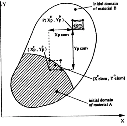
the Eulerian method is a special case with fixed nodal points. As illustrated in Figure

3.1, the displacement of nodal point N is given by Ax/N. The displacement of the

material point that coincides with nodal point N at the beginning of the step is

represented by AuaN. The difference between the new locations of the nodal point N

AyN =AX7-Au (3.21)

The new location (at time t + At) of a material point B, which coincides with an integration point A of an element at time t, is found by:

x,(B)= x,(A)+ V/ N (Xi(A))*AU N

The new location of the corresponding integration point C, is:

x,

(C)

Now the stresses and strains at the new integration points (points like C) need to be determined. The stresses at material point B can be calculated in the same way as in the Lagarangian procedure:

t+Az

au (B)= W+f,(A)+ fdt (3.24)

where 6. is determined from Equation (3.7). The stresses at the new integration point

C are found by:

CU (C)= 0 (B)+ 0%k (B)Ayk + O(Ayk )2 (3.25)

The difference between stresses at point B and point A is of order AuaN. And,

AyN and Au/N are of the same order. Therefore, Equation (3.25) can be written as:

U, (C)=

0

(B)

To calculate the covariant derivative of stress, 0%,k' in Equation (3.26), the

are calculated as an average from all elements that are connected to the nodal point.

After that, an additional stress field at time t within an element is defined as:

Ui* (X'k)=NX k ti

(3.27)

where, the superscript "t" is the current time step, the asterisk at the left side means

these stresses are introduced and do not exactly coincide with stresses at the

integration points. U';N i stress at nodal point at time t.

With Equation (3.27), the derivative of the stresses is 1st order approximated

by:

a

(3.28)

Substituting Equation (3.28) into (3.26) and neglecting higher order terms of

Ayk, results in the stresses at the new integration points:

j- (C) = UY (B)

o>(C)

The strains at the new integration points can be solved in the same way. If the nodal

N

point displacements are chosen to be equal to the material displacement, i.e., Ayi _

0, Equation (3.29) yields:

-ij

(C)=

It reduces to a Lagarangian procedure, which has element nodes and material points

coupled.

For Eulerian procedure, the nodes are fixed in space, i.e., AyN = -AUN. If this

,(C)= U4 (B)- aNNV M (3.31) The second item in the right side of Equation (3.31) is the so-called convection item. In the Eulerian formulation, point C is the same as point A, since the nodal points do not move. Combining with Equation (3.24), Equation (3.31) can also be written in a more general format as:

t+At

07 (x,t + At)=

a

where x is the coordinate for A, or the fixed nodal point.

Huetink (1986) observed that this formulation gave numerical instabilities depending on the size of the displacement increments. In order to avoid instabilities, the following equation is introduced by Huetink (1986):

0'jj(x, t+ At)=07y(x -Au~t)+ t+Afddt (3.33)

where Au is the displacement of the material particle, which originally coincides with the nodal point, during time increment At. It should be pointed out that Equation

(3.32) is a first-order spatial Taylor series expansion of Equation (3.33). Huetink

(1986) observed that using Equation (3.33) results in numerical diffusion (i.e., over

smoothing). Equation (3.32) is an element solution, while Equation (3.33) is a nodal solution. If the continuous field is made by averaging in the nodes, the peaks in the solution will be averaged out. This is numerical diffusion. On the other hand, if only the element gradient is taken and no average on the nodes, the solution becomes

unstable and starts to oscillate. Therefore, in the present implementation, a weighted

sum of Equation (3.32) and (3.33) is adopted, as follows:

t+At

ai- (x, t + At)= (1 - a a- (x, t) + fd-,jdt + au-,(x - Au, t)

-(-a)[VN X,k t' N xAu (3.k4 As Van den Berg (1996) suggested, "a reasonable range for a appears to be":

Au < a 2 _(3.35)

le _le

where le represents the element length. In the finite element program DiekA, the

weight factor a is automatically taken into account at the element level. The weight

factor depends on the convective displacements, compared to the element size (the

Courant number), as shown in Equation (3.35). In case of small Courant numbers,

mainly the element solution (Equation (3.32)) is taken. Otherwise, the solution is

more close to the nodal solution (Equation (3.33)).

3.3

Layered Deposits with Eulerian Approach

The geology of the subsoil generally consists of layered deposits. With Eulerian

approach, modeling the penetration process in layered deposits requires that the

material particles stream through the fixed mesh including its constitutive behavior. In

DiekA, an extra state variable, material index, is assigned to each integration point, to

store the material type associated with the node.

For analysis with layered soils, at the end of each increment, following the