On noise prediction in maps obtained with global DIC

HAL Id: hal-01163331

https://hal.inria.fr/hal-01163331

Submitted on 19 Nov 2015

HAL is a multi-disciplinary open access

archive for the deposit and dissemination of

sci-entific research documents, whether they are

pub-lished or not. The documents may come from

teaching and research institutions in France or

abroad, or from public or private research centers.

L’archive ouverte pluridisciplinaire HAL, est

destinée au dépôt et à la diffusion de documents

scientifiques de niveau recherche, publiés ou non,

émanant des établissements d’enseignement et de

recherche français ou étrangers, des laboratoires

publics ou privés.

On noise prediction in maps obtained with global DIC

Benoît Blaysat, Michel Grediac, Frédéric Sur

To cite this version:

Benoît Blaysat, Michel Grediac, Frédéric Sur. On noise prediction in maps obtained with global DIC.

SEM Annual Conference & Exposition on Experimental and Applied Mechanics - 2015, SEM, Jun

2015, Costa Mesa, CA, United States. pp.211-216, �10.1007/978-3-319-22446-6_27�. �hal-01163331�

ON NOISE PREDICTION IN MAPS OBTAINED WITH GLOBAL DIC

B. Blaysat

, M. Grédiac

, F. Sur

1

Clermont Université, Université Blaise Pascal, Institut Pascal, UMR CNRS 6602

BP 10448, 63000 Clermont-Ferrand, France

2

Laboratoire Lorrain de Recherche en Informatique et ses Applications, UMR CNRS 7503

Université de Lorraine, CNRS, INRIA projet Magrit, Campus Scientifique, BP 239

54506 Vandoeuvre-lès-Nancy Cedex, France

ABSTRACT

A predictive formula giving the measurement resolution in displacement maps obtained using Digital Image Correlation was proposed some years ago in the literature. The objective of this paper is to revisit this formula and to propose a more general one which takes into account the influence of subpixel interpolation for the displacement. Moreover, a noiseless DIC tangent operator is defined to also minimize noise propagation from images to displacement maps. Simulated data enable us to assess the improvement brought about by this approach. The experimental validation is then carried out by assessing the noise in displacement maps deduced from a stack of images corrupted by noise. It is shown that specific image pre-processing tools are required to correctly predict the displacement resolution. This image pre-processing step is necessary to correctly account for the fact that noise in images is signal-dependent, and to get rid of parasitic micro-movements between camera and specimen that were experimentally observed and which corrupt noise estimation. Obtained results are analyzed and discussed. Keywords: digital image correlation, displacement, full-field measurement, metrological performance, resolution

INTRODUCTION

Full-field measuring tools like DIC have recently spread in experimental mechanics thanks to the wealth of data they provide, and also thanks to the constant decrease of camera and computer cost. Indeed, it is possible to measure the displacement fields on the surface of specimens while testing and to deduce the corresponding displacement fields. This is very useful in many cases of material and structure characterization.

Any measuring tool must be characterized in terms of metrological performance. However, no standard is available for full-field measurement methods. Their metrological performance depends however of their measurement resolution, and of other parameters such as the spatial resolution and the bias [1]. We focus here only on the first parameter. It is defined in Ref. [1] by the smallest change in a quantity being measured that causes a perceptible change in the corresponding indication. This can be interpreted here as the standard deviation of the noise in the displacement maps, as proposed in [2] for instance. Following previous studies on noise in displacement maps obtained by DIC [3-4], a formula predicting the displacement resolution has been given in [5]. We propose first a more general formula which takes into account the influence of subpixel interpolation for the displacement. We also used a noiseless DIC tangent operator to minimize noise propagation from images to displacement maps. This formula and the assumptions under which it is obtained are given in the first section of the paper. It is then validated using simulated noisy data. The practical comparison between predicted and experimental resolutions is only scarcely addressed in the literature. In this context, we performed experiments aimed at estimating the experimental resolution through a stack of images. The obtained results are presented in the third section of the paper. Since poor results

were obtained, we investigated the possible physical causes, and proposed suitable pre-processing tools of the images to counterbalance the two effects that were identified, namely sensor noise heteroscadasticity and micro-movements between camera and specimen. These tools are briefly discussed in the fourth section of the paper. We finally measured the displacement resolution obtained from on these pre-processed images and we can conclude that the proposed predictive formula is observed satisfied.

PREDICTIVE FORMULA FOR THE DISPLACEMENT AND STRAIN RESOLUTIONS ACCOUNTING FOR THE SUB-PIXEL INTERPOLATION

In Ref. [5], it is proposed to predict the displacement resolution obtained in global DIC [4]. In this case, the output of the DIC procedure is a set of degrees of freedom (DoFs), from which the displacement can be reconstructed at any point by relying on

the shape functions that define the kinematics. The “classic” predicted value p

i   reads as follows:

 

- _fis the standard deviation of the noise in the images

- [M1]_iiis the iith component of the DIC tangent operator. By definition, it is such that M=Jt.J with J the Jacobian of the DIC residual

- _iis the ith DoF. These DoFs govern the displacement map.

We recently proposed to account for the sub-pixel interpolation of the displacement in this prediction, which leads to another

quantity denoted p i   [6]:

 









- AM1Jt, and A is such that A.At=M-1

- P is the subpixel interpolation matrix. It is such that P.Pt=I only when the displacement is equal to an integer number of pixels. In this case, Equation (2) obviously reduces to Equation (1)

The equations above are obtained under the following assumptions:

- the noise corrupting the processed images is assumed to be a Gaussian white noise, and its standard deviation is the

same at any pixel. Such a noise is referred to as homoscedastic

- during the optimization procedure employed in DIC, the modified Gauss-Newton scheme is adopted, so we assume

that the perturbation of the DoFs is small enough with respect to the optimized DoF values themselves

- the image gradients of both the reference and the current images processed by DIC are identified with their noiseless

counterparts, which can be obtained for instance by averaging a stack on images of the initial configuration

- P in Equation (2) is the matrix obtained once convergence is reached.

Full details on the elaboration of these predictive formulas can be found in [6].

VALIDATION OF THE PREDICTIVE FORMULAS WITH SYNTHETIC DATA

The validity of these two predictive equations has first been assessed thanks to simulated data. A self-rotation around the center of a synthetic randomly marked surface has been considered. A white noise of standard deviation _f = 400 gray levels has been added to the gray levels of the synthetic images of the surface encoded on a bit-depth of 216 bits. This is a typical value for CCD cameras, as measured in [7] for instance. 100 images affected each by a different copy of the noise

were considered and the empirical displacement resolution has then been characterized at any DoF of the mesh employed in

the DIC procedure. This mesh contains 61x61 elements. Each element covers a 13x13-pixelzone. The maximum value for

the norm of the displacement along the borders of the region of interest is 2.5 pixels. This value enables us to check the efficiency of both the classic and new formulas over a wide range of sub-pixel displacements. This parameter has indeed been observed to influence the obtained results, as predicted by Equation (2).

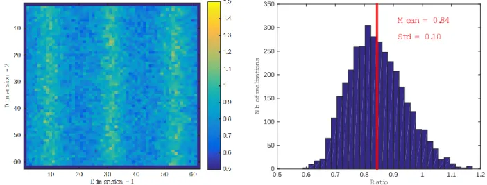
Figure 1 shows a typical distribution of the ratio between predicted and empirical values for the displacement resolution along the y-direction (similar results are obtained along the x-direction). This ratio is calculated at each DoF of the mesh. We consider in turn the ratio obtained with Equation (1) for the prediction (results are shown in Figure 1), and then with Equation (2) (see results in Figure 2).

Figure 1. Ratio between predicted and observed resolutions, Equation (1) being considered for the prediction. Left: distribution of the ratio at the DoFs. Right: histogram of this ratio.

Figure 2. Ratio between predicted and observed resolutions, Equation (2) being considered for the prediction. Left: distribution of the ratio at the DoFs. Right: histogram of this ratio. Same colorbar as in Figure 1.

The following conclusions can be drawn:

- Equation 1 provides a reasonable global assessment for the displacement resolution since on average, there is a 16%

difference with the experimental resolution;

R atio 0.5 0.6 0.7 0.8 0.9 1 1.1 1.2 N b of re al is at io n s 0 50 100 150 200 250 300 350 M ean = 0.84 Std = 0.10 R atio 0.5 0.6 0.7 0.8 0.9 1 1.1 1.2 N b of re al is at io n s 0 50 100 150 200 250 300 350 M ean = 0.96 Std = 0.06

- Equation 2 gives on average a predicted displacement resolution closer to the experimental one since the difference is only equal to 4%. The distribution is also less spread compared to the preceding one, as also illustrated by the standard deviation which is lower than in the preceding case;

- In both cases, the maximum difference between predicted and experimental resolutions is reached along vertical lines which correspond either to integer values for the displacement, or to maximum sub-pixel displacements.

VALIDATING THE PREDICTIVE FORMULAS WITH EXPERIMENTAL DATA

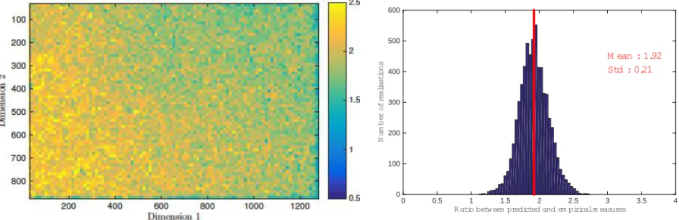
The objective here is to check the validity of the formulas through a set of images shot during a mere translation test. The first tested specimen was randomly marked. A displacement equal to 2.5 pixels was applied with a testing machine. The lighting was deliberately heterogeneous, with only one light source placed near the bottom left-hand side of the specimen. The objective here is to check also the influence of this parameter, because it is expected to influence the results [7]. 100 images were shot in both the reference and the current configurations. The regular mesh used to process the images has here 97x66 elements, and the surface of each element is again 13x13 pixel2. Figure 3 shows the ratio obtained in this case between predicted and empirical resolutions.

Figure 3: Ratio between predicted and observed resolutions, Equation (2) being considered for the prediction. Left: distribution of the ratio at the DoFs. Right: histogram of this ratio.

The most stricking remark is the fact that on average, this ratio is much greater than 1. It means that apparently, Equation (2) is unable to predict correctly the real displacement resolution. Equation (1) does not provide either a better prediction (results not reported here). The first reason explaining this bad result is the fact that the standard deviation for the noise in the images

f

 is not constant throughout the images. It is indeed well-known that this standard deviation strongly depends on the brightness: the variance is an affine function of the brightness [8,9]. Real noise is therefore not homoscedastic, but signal-dependent, or heteroscedastic. In addition, real noise in cameras is generally not Gaussian but Poisson-Gaussian. Correcting the difference between real noise and model noise used in both the formulas is possible by applying the so-called Generalized Anscombe Transform (GAT) which transforms a heteroscedastic Poisson-Gaussian noise in a homoscedastic Gaussian one. This transform requires to know some characteristics of the camera which were identified here in a separate study [7,10]. Applying the GAT to the images and then processing the resulting images to retrieve the displacement leads to the results presented in Figure 4. Interestingly, the scatter is much lower compared to the preceding histogram. We can also see that the resolution distribution still depends on the lighting intensity, which illustrates that the GAT did not perfectly work here since this distribution should have become homogeneous after applying this transform. Another problem is that the mean value for the resolution does not change and is still much greater than one. These two observations mean that a phenomenon other than heteroscedasticity occurs.

The reason for the aforementioned problems is that micro-movements between camera and specimen occurred while taking the set of 100 images: the testing machine and the tripod of the camera did not remain on a strong floor, as in many labs, and thus tiny low-frequency movements were observed in a repeatable fashion. They did not induce any blurring in the images because of their low frequency (order of magnitude: about 0.1 Hz): the corresponding period is much higher than the shutter

R atio between predicted and em piricalm easures

0 0.5 1 1.5 2 2.5 3 3.5 4 N u m b er of re al is at io n s 0 100 200 300 400 500 600 700 M ean : 1.91 Std : 0.40

time of the camera. However, their amplitude, even tiny (between one and two micrometers), is not negligible compared to the size of the region observed by any pixel of the camera sensor, which equals about 40 micrometers.

Figure 4: Ratio between predicted and observed resolutions, Equation 2 being considered for the prediction. The images were pre-processed with the GAT. Left: distribution of the ratio at the DoFs. Right: histogram of this ratio.

When analyzing the set of 100 images, these microvements induce an apparent noise which causes the apparent noise in the images to be greater than the one only caused by the camera sensor. Correcting this phenomenon directly on the images is possible, but a non-local averaging procedure must be applied before retrieving the displacement. This procedure has been developed only in the case of regular marking like grids [10]. It is not yet available for markings different from regular ones. We therefore decided to perform the same experiment as the preceding one on a specimen marked with a bidirectional grid (pitch 0.2 mm, thickness of the lines: 0.1 mm). In particular, the lighting source was still placed near the bottom left of the specimen to insure a heterogeneous lighting intensity in the grid images, and thus a heterogeneous noise variance. It is worth mentioning that performing DIC in regular marking is possible, albeit not really usual. This only requires certain precautions when initiating the iterative procedure, for instance by using a pyramidal approach [11].

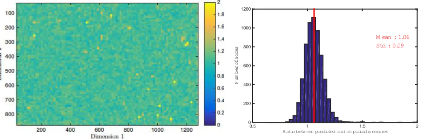
The results obtained in this case are shown in Figure 5. It can be seen that the displacement resolution is now nearly homogeneously spatially distributed despite the strongly heterogeneous lighting. The mean value for the ratio is now very close to 1: we only slightly overestimate (6%) the prediction, thus illustrating the efficiency of Equation (2), even for a subpixel displacement which is maximum (0.5 pixel). Full details on these experiments and as well as additional results are available in [12].

CONCLUSION

Sensor noise propagation between images and final displacement maps was studied in this paper to predict resolution in displacement maps obtained by global DIC. An improved version of the predictive equation for the displacement resolution available in the literature was proposed. It mainly accounts for the sub-pixel part of the displacement, which is shown to influence the resolution. Simulated data illustrate the improvement brought about by this new predictive formula. Performing the experimental verification is trickier. Indeed two phenomena corrupted the experiment: i- micro-movement between camera and specimen which occurred when capturing a set of images to assess the noise level in images; and ii- noise heteroscedasticity, which led one of the assumptions under which the predictive formula is elaborated not to be satisfied. Both these problems were resolved by considering suitable pre-processing procedures, namely the so-called Non Random Signal Reduction for the first problem, and the Generalized Anscombe Transform for the second one. The first pre-processing can however only be applied on regular markings, which led us to perform the experiments on regularly marked surfaces, namely grids. This finally leads the predictive formula to be satisfactorily verified.

R atio between predicted and em piricalm easures

0 0.5 1 1.5 2 2.5 3 3.5 4 N u m b er of re al is at io n s 0 100 200 300 400 500 600 M ean : 1.92 Std : 0.21

Figure 5: Ratio between predicted and observed resolutions, Equation 2 being considered for the prediction. The surface is here regularly marked with a grid. The images were pre-processed with the GAT. Left: distribution of the ratio at the DoFs. Right: histogram of this ratio.

REFERENCES

[1] JCGM. International vocabulary of metrology – Basic and general concepts and associated terms (VIM), volume 200. BIPM, 2012.

[2] A. Chrysochoos and Y. Surrel, Basics of metrology and introduction to techniques, Chapter one ; pages 1-29, in Full-field

measurements and identification in solid mechanics, edited by M. Grédiac and F. Hild, Wiley, 2012

[3] Z. Y. Wang, H. Q. Li, J. W. Tong and J. T. Ruan. Statistical analysis of the effect of intensity pattern noise on the displacement measurement precision of digital image correlation using self-correlated images. Experimental Mechanics 47(5):701–707, 2007.

[4] G. Besnard, F. Hild, and S. Roux. Finite-element displacement fields analysis from digital images: application to Portevin-Le Châtelier bands. Experimental Mechanics, 46(6):789–803, 2006.

[5] J. Réthoré, G. Besnard, G. Vivier, F. Hild, and S. Roux. Experimental investigation of localized phenomena using digital image correlation, Philosophical Magazine, 88(28-29): 3339–3355, 2008.

[6] B. Blaysat, M. Grédiac and F. Sur, The effect of interpolation in noise propagation from images to DIC displacement maps, submitted, 2015

[7] M. Grédiac and F. Sur, Effect of sensor noise on the resolution and spatial resolution of the displacement and strain maps obtained with the grid method, Strain, 50(1): 1-27, 2014

[8] A. Foi, M. Trimeche, V. Katkovnik and K. Egiazarian, Practical Poissonian-Gaussian noise modeling and fitting for single-image raw-data, IEEE Transactions on Image Processing, 17(10): 1737-1754, 2008

[9] G.E. Healey and R. Kondepudy, Radiometric CCD camera calibration and noise estimation, IEEE Transactions on

Pattern Analysis and Machine Intelligence, 16(3): 267-276, 1994.

[10] F. Sur and M. Grédiac, Sensor noise modeling by stacking pseudo-periodic grid images affected by vibrations, IEEE

Signal Processing Letters, 21(4): 432-436, 2014

[11] R. Fedele, L. Galantucci, and A. Ciani. Global 2D digital image correlation for motion estimation in a finite element framework: a variational formulation and a regularized, pyramidal, multi-grid implemen- tation. International Journal for Numerical Methods in Engineering, 96(12):739–762, 2013.

[12] B. Blaysat, M. Grédiac and F. Sur, On the propagation of camera sensor noise to displacement maps obtained by DIC – an experimental study, submitted, 2015

R atio between predicted and em piricalm easures

0.5 1 1.5 2 N u m b er of n o d es 0 200 400 600 800 1000 1200 M ean : 1.06 Std : 0.09