Black into green: A BIG opportunity for
North Dakota’s oil and gas producers
The MIT Faculty has made this article openly available.
Please share
how this access benefits you. Your story matters.
Citation
Taylor, David D. J. et al. "Black into green: A BIG opportunity for
North Dakota’s oil and gas producers." Applied Energy 242 (May
2019): 1189-1197 © 2019 The Authors
As Published
http://dx.doi.org/10.1016/j.apenergy.2019.03.158
Publisher
Elsevier BV
Version
Final published version
Citable link
https://hdl.handle.net/1721.1/127204
Terms of Use
Creative Commons Attribution 4.0 International license
Contents lists available atScienceDirect
Applied Energy
journal homepage:www.elsevier.com/locate/apenergy
Black into green: A BIG opportunity for North Dakota’s oil and gas producers
David D.J. Taylor
a,1, Mariya Layurova
a, David S. Vogel
b,c, Alexander H. Slocum
a,⁎aMassachusetts Institute of Technology, 77 Massachusetts Ave., Cambridge, MA 02139, United States bVoloridge Investment Management, Jupiter, FL 33477, United States
cVoLo Foundation, Jupiter, FL 33468, United States
H I G H L I G H T S
•
The business inertia of hydrocarbon production can accelerate wind energy production.•
Emissions-to-price ratio makes BIG funding feasible for oil and natural gas in ND.•
BIG’s wind farm is funded from 10% of hydrocarbon revenues and $0.03/kWh of wind power.•
Over 40 years, ND’s oil and gas can fund 89,000 wind turbines, generating 155GW.•
This wind power offsets 100% of the well-to-wheel emissions of ND’s oil and gas. A R T I C L E I N F O Keywords: GHG emissions Wind turbines North Dakota Shale oil Natural gas A B S T R A C TA new perspective on carbon economics is developed and applied to demonstrate that oil and natural gas producers in North Dakota (ND) have an opportunity to make a profitable transition to wind energy producers. ND’s oil and gas producers can fund this black into green (BIG) transition by: first, investing a fraction of their revenues into wind energy farms; and second, reinvesting a portion of revenues from the wind-generated electricity. Over a period of 40 years, 100% of the greenhouse gas emissions associated with the production and consumption of ND’s oil and gas could be offset with an investment of 10% of both hydrocarbons’ value and a reinvestment of three cents per kilowatt-hour of wind-generated electricity. At the end of the 40-year period, the resultant 155-gigawatt wind farm would have offset 13.4 × 10⁹tons of carbon dioxide equivalent and cost
$9.90/ton of offset carbon dioxide equivalent. This BIG example demonstrates the financial and environmental benefits of ND’s oil and gas producers transforming into renewable energy producers; hence regulators, hy-drocarbon producers, and utilities should take note and think BIG. The reconfigurable, Excel-based model used herein is provided to allow readers to extend this example from ND to other regions, hydrocarbons, and green energy sources.
1. Introduction
Climate change and global warming are estimated to put between $2.5 and $24 trillion of global assets at risk[1]. Action to reduce our current greenhouse gas (GHG) emissions is urgently required [2–4]. Delaying our collective climate action will increase the costs of miti-gation, increase the costs associated with fossil fuel reserves that will have to be abandoned, and worsen the economic slowdown induced by climate action[2,3].
International consensus has been building that global warming should be limited to well below 2 °C warmer than pre-industrial tem-peratures[5–7]. To meet such targets, some economically recoverable
reserves of fossil fuels, especially coal, must remain unused [8–10]. 63% of anthropogenic carbon emissions since 1854 can be traced to 90 corporations [11]. Historically, these corporations have coordinated their resistance to environmental policies and especially to a global carbon tax[12–14]; the stronger a country's energy-intensive industries are, the more likely it is to have weaker environmental regulations [14]. Workers, unions, regions, and firms who depend on the existing production systems are understandably concerned about how dec-arbonization will affect their livelihoods [15–17]. Such concerns are unified by narratives like ‘jobs vs. environment’[15,16]and are most polarizing in regions in which the costs of climate mitigation will be concentrated. But ‘jobs vs. environment’ is a misleading dichotomy.
https://doi.org/10.1016/j.apenergy.2019.03.158
Received 1 December 2018; Received in revised form 2 March 2019; Accepted 16 March 2019
⁎Corresponding author.
E-mail address:slocum@mit.edu(A.H. Slocum).
1Present address: University of Toronto, 55 George St., Toronto, ON M5S 0C9, Canada.
Available online 23 March 2019
0306-2619/ © 2019 The Authors. Published by Elsevier Ltd. This is an open access article under the CC BY license (http://creativecommons.org/licenses/BY/4.0/).
Taylor et al.[18]introduced the idea that oil producers in Alberta could transition to become wind energy producers if they were required to invest in wind energy in parallel with their oil extraction. In such a case, decarbonization would occur within existing firms in the same region as traditional extraction sites. Accordingly, many of the concerns of the workers, unions, regions, and firms (and their shareholders) would be appeased. The idea of Taylor et al.[18], however, with cur-rent weather patterns and hub height technologies, was not viable in Alberta due to low wind speeds. Yet solutions that blend technology, policy, and market forces have the potential to overcome the economic, social, and technical systems that reinforce our current, carbon-in-tensive economy[12,19–22].
Given the importance of carbon-producers in emitting GHGs and shaping climate policy, we adapt the initial idea of Taylor et al.[18] and consider a Black Into Green (BIG) opportunity for firms to reduce their net GHG emissions. To do so, hydrocarbon producers i) invest a fraction of their hydrocarbon (black) revenues into producing wind (green) energy, and ii) reinvest a portion of the wind-energy revenues into further expanding wind-energy production.
The success of either a carbon tax or a cap-and-trade system de-pends more on the details of its implementation than the choice be-tween systems[23–25]. In this paper, we assume that either a carbon tax or a cap-and-trade system has been imposed and that it is based on a firm’s net GHG emissions. Under such a system, firms have an incentive to reduce their net GHG emissions, provided that such reductions are cheaper than the costs associated with the carbon tax or cap-and-trade system. Thus, a BIG approach would allow firms to keep what they would have paid under either system as an asset on their balance sheets, increasing their long-term business prospects. This paper develops a method for quantifying the minimum GHG-emissions penalty (asso-ciated with either a carbon tax or a cap-and-trade system) required to incentivize hydrocarbon producers to participate in the proposed BIG approach. By participating, firms avoid paying a carbon penalty, and instead build greater long-term value for their companies.
To evaluate the initial feasibility of BIG, we apply BIG in North Dakota (ND) as an example, since ND has substantial wind, oil, natural gas, and coal resources[26]. The shale oil in ND’s Bakken formation is the largest known source of oil in the United States (U.S.) [27]. Leveraging this resource to stimulate green energy production will be critical in shaping the U.S.’ energy mix and environmental footprint. Over 20% of U.S.'s total emissions come from fossil fuels extracted on federal land[28], providing the government with a unique opportunity to influence the trajectory of this emissions source[28,29]. Yet con-cerningly, fossil fuel extraction on from federal lands is increasing, not decreasing[30].
This paper first considers the potential for BIG to offset the GHG emissions associated with the production and consumption of ND’s hydrocarbons. Second, this paper quantifies what investment and re-investment rates are required to achieve these GHG offsets. Finally, the financial efficiency of BIG’s GHG-mitigation is compared to California’s cap-and-trade price (2014–17 average of $13/ton of carbon dioxide equivalent (t CO2e)[31]) and the price of voluntary emission offsets in
North America (average $2.9/t CO2e in 2016[32]).
Due to the sometimes-contentious nature of combing hydrocarbon and green energy production, this paper uses a transparent and re-configurable Excel-based model. Readers wishing to investigate results with different inputs or assumptions are encouraged to download the model from theSupplemental Materials (SM), SM-Model 1. With a view of short- and long-term success for all, this paper’s BIG proposal sug-gests a potential mechanism to transform ND’s energy production landscape, benefit climate and environmental outcomes, and maintain the livelihoods of workers, unions, regions, and firms dependent on hydrocarbon production.
2. Methods
The viability of this BIG proposal depends on: (i) the GHG-intensity of hydrocarbon production and consumption, (ii) the availability of wind power, (iii) the ability for wind-generated electricity to offset GHG emissions, and (iv) the feasibility of the funding scheme. This section explains each of these model components and the metrics used to quantify BIG’s efficacy and financial efficiency. BIG’s performance was assessed over a 40-year time horizon and across the state of ND.
While a multitude of methods exist for detailed evaluations of clean energy policies[33], we present a deterministic (and positivist), tech-noeconomic model[34,35]of how our proposed investment structure could influence the cumulative emissions associated with ND’s oil and gas production. This first-order analysis aims to demonstrate that en-ergy producers should consider simultaneous investments into clean energy production as a liability reduction strategy in the presence of carbon-penalizing regulations. Given the polarized nature of current policy debates, we submit that a simpler, more transparent model provides decision makers better insights amidst modeling uncertainties [36].
Before a BIG proposal is actually implemented, our first-order analysis should be supplemented with more detailed studies that in-clude social and political dynamics, implementation details, and market responses to the BIG proposal[34]; the results of said studies should be used accordingly to evolve the first-order model of the BIG idea pre-sented in this paper.
2.1. GHG emissions of hydrocarbon production in North Dakota To account for the GHG emissions associated with oil, gas, and coal extraction, the metric of carbon dioxide equivalent (CO2e) per gigajoule
(GJ) of thermal energy was used. For energetic conversions, the lower heating value was used throughout this paper. The GHG emissions of each hydrocarbon are summarized inTable 1and were accounted for using two categories:
1. production emissions: the total GHG emissions caused by producing, upgrading, refining, and transporting the hydrocarbon (i.e., well-to-tank); and
2. total emissions: the total GHG emissions caused by all steps from production through end consumption of the hydrocarbon (i.e., well-to-wheel/combustion).
The production and total emissions of shale oil were estimated to be 21.4 and 94.6 kg CO2e/GJ, respectively[37](Table 1). Production and
total emissions of ND’s natural gas (shale gas) were estimated to be 14.6 and 70.9 kg CO2e/GJ, respectively [38](Table 1). Finally, the total
emissions of ND’s lignite coal was estimated to be 116 kg CO2e/GJ[39],
4% of which (4.64 kg CO2e/GJ) is due to production[40](Table 1). The
rationale for selecting these specific emissions references is detailed in Section SM-1.Table 1also includes the 2017 prices for oil, natural gas, and coal that were used in this study.
Table 1
ND’s shale oil, natural gas (shale gas), and (lignite) coal emissions, prices, and production rates. Units of gigajoule (GJ) refer to thermal energy.
Production emissions (kg CO2e/GJ) Total emissions (kg CO2e/GJ) Price in 2017 ($/GJ) Production in ND (109GJ/year) Shale oil 21.4[37] 94.6[37] 8.87[44] 2.28[41] Shale gas 14.6[38] 70.9[38] 3.98[45] 0.72[42] Lignite coal 4.64[39,40] 116[39] 1.52[46] 0.41[43]
D.D.J. Taylor, et al. Applied Energy 242 (2019) 1189–1197
The annual production in ND was estimated in 2017 to be 2.28 billion GJ of oil (388.3 million barrels) [41]and 725 million GJ of natural gas (687.1 billion cubic feet)[42]. Production of coal was es-timated using the 2016 gross production value of 414 million GJ (392 trillion Btu)[43]. A constant growth rate of 1% for oil, natural gas, and coal production was assumed in the BIG model to ensure its conclusions do not rely on artificially-high projected growth rates.
2.2. Wind power generation
Two options were considered for the allowable size of the BIG-funded wind farm: first, wind turbines were allowed throughout ND (area of 178,111 km2[47]); second, wind turbines were limited to ND’s
oil-producing counties (39% of ND; 68,600 km2 [48]). As in Taylor
et al.[18], the maximum wind turbine density was set as one turbine per km2. Moreover, for a given land area, only half of it was assumed to
be feasible for turbine siting (net density of 0.5 turbines per km2).
Wind speed distributions at 80 m above ground[49]were spatially averaged using ImageJ [50]. RETScreen was used to convert these average wind speeds into capacity factors using turbine power-curve data [51]and a wind-shear exponent of 0.2 [52]. The Vestas V126 3.45 MW turbine was selected as a reference turbine, however, because more detailed power-curve data was available for the V126 3.3 MW version, the latter’s data was used to calculate the capacity factor.
The state of ND and its oil-producing counties were found to have average capacity factors of 50.5% and 51.5%, respectively (details in Section SM-2). The calculated capacity factors are higher than more general estimates of the wind capacity factor in the U.S. interior (e.g., Wiser et al.’s estimate of 42.7% [53]), because of the slower wind speeds in the U.S. interior and older turbine models used in such stu-dies. Capacity factors of 50.5% and 42.7% are considered in the results below. Turbine sizes and hub heights have increased over time and such new technology developments continue to increase capacity factors and the potential of BIG.
Installed wind turbines were conservatively estimated to have a life expectancy of 20 years [54]. Turbine capital and maintenance costs were approximated as $1.71 per watt (W) [55]and $0.031/W/year [56], respectively. GHG emissions associated with wind-generated electricity were estimated to be 10.4 g of CO2e per kilowatt hour of
wind-generated electricity (kWhwind)[57].
2.3. GHG-emission offsets from wind-powered electricity generation Electricity production from wind power only reduces net GHG emissions when a generation technology that emits more GHG than wind is turned off. In the case of this first-order model, the generation technology that would be turned off was assumed to have the average GHG intensity of the region to which the wind power was transmitted. Additional transmission lines for the wind power were estimated to cost $372/MW/km[58](the mid-point estimate of Delucchi and Jacobson [58], whose low and high estimates were $299-$429/MW/km). The transmission system was assumed to have a 40-year life expectancy (an average life expectation for transmission line components) [58]. Transmission losses were approximated as 1.5% + 1%/1000 km of average power, following Delucchi and Jacobson[58].
The GHG intensity of the electricity grid is segmented by the Environmental Protection Agency (EPA) into 26 “eGRID subregions” [59]. The BIG model considers sending wind-generated electricity to the closest 20 subregions, including North Dakota’s (“MRO West”; Fig. 1). Subregional capacities, generation mixes, and GHG intensities are accounted for in the BIG model and summarized inSection SM-3.
The BIG model dispatches electricity to the different eGRID sub-regions according to a user-definable transmission priority. When one subregion reaches its maximum capacity for wind power, assumed to be 20% of produced power (not generation capacity) [61], the model builds transmission lines to the next prioritized subregion. The default
transmission priority (SM-Table 2) was set by GHG intensity. 2.4. Funding mechanism
Different investment and reinvestment combinations were ex-amined to show their influence on GHG emissions and financial effi-ciency. Typical electricity-utility profit margins in the U.S. range from 6 to 15%[62], but these include capital and maintenance costs, which are accounted for in our BIG model. Accordingly, as a first approximation, the maximum reinvestment rate was considered to be 25% of the average electricity price in the U.S. ($0.12/kWh[63]), equivalent to a maximum reinvestment rate of $0.03/kWhwind. Conservatively setting
this maximum reinvestment rate ensures that hydrocarbon producers would have an incentive to keep their wind turbines operating at their full potential.
2.5. Big’s performance metrics
Predicted peak global warming values are strongly correlated with cumulative emissions of carbon[64]. Focusing on cumulative emis-sions, instead of annual emisemis-sions, simplifies policy discussions and makes policies more robust to the uncertainties in climate models[64]. Financial investments in infrastructure, resource extraction, and re-source exploration implicitly commit to the use of those investments far into the future[65–67]. By considering the cumulative emissions of those investments, the total climate impacts of current investments can be quantified[65–67].
Cumulative, offset GHG emissions were used to assess the efficacy of BIG. These offsets were compared to the cumulative emissions asso-ciated with the extracted hydrocarbon(s) used to fund BIG. The goal of BIG could be to offset 100% of the cumulative total emissions or the cumulative production emissions of the associated hydrocarbon(s). For example, if BIG were funded by oil and gas production in ND for 40 years, it would be reported to have offset 100% of the total emissions of oil and gas if the sum of all GHG offsets from the wind farm earned over 40 years equaled the sum of all GHG emissions from the produc-tion and consumpproduc-tion of ND’s oil and gas over that same time horizon. No discounting factor was used to distinguish between future and present GHG emissions.
The financial efficiency of BIG was considered as the equivalent cost per ton of offset GHG emissions, calculated as the net present cost of all expenditures divided by the total offset GHG emissions. Two discount rates were compared in the model: the mean industry-specific discount rate (7%[68]), and, to be conservative, 3% (a higher discount rate improves the favorability of BIG).
3. Results
3.1. Emissions-to-price ratio is key to BIG’s viability
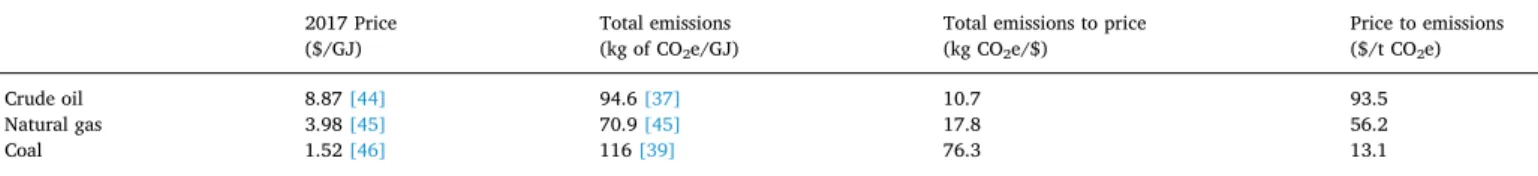
BIG is initially funded by a fixed percentage of revenues from the sale of hydrocarbons. BIG’s ability to offset GHG emissions, therefore, depends on the ratio of total GHG emissions to price for each hydro-carbon (Table 2). In an extreme example, if offsetting GHG emissions costs more than the price of a hydrocarbon, it becomes cheaper to forgo burning the hydrocarbon (this occurs at $13.1/ton of CO2e for coal;
Table 2). Coal emits seven times more GHGs than oil on an equal-price basis (Table 2). Natural gas emits four times less than coal, but 67% more than oil, again on an equal-price basis (Table 2).
BIG models of each hydrocarbon individually showed that BIG was only viable for ND’s oil and gas industries (coal required an investment rate of 43% to offset its total emissions,Section SM-4). Accordingly, the results that follow model a combined BIG scenario that offsets ND’s oil and gas (but not coal) emissions.
3.2. Cumulative efficacy and financial feasibility
If wind turbine installations are limited to oil-producing counties (39% of ND’s area), area is a limiting constraint and only 69% of the total emissions from ND's oil and gas can be offset (Section SM-5 and SM-Fig. 1). However, if the area allowed for the wind farm is increased to the whole state of ND (still assuming only half is viable for siting a wind turbine), offsetting 100% of the total emissions from oil and gas is feasible with different combinations of investment and reinvestment rates. Minimum combinations of investment and reinvestment rates
form the curves plotted inFig. 2, which depend on the capacity factor and if BIG’s goal is to offset 100% of oil and gas’ production emissions or 100% of their total emissions.
With a capacity factor of 50.5% (results assuming a 42.7% capacity factor are shown in parentheses) and without reinvestment, offsetting 100% of total emissions would require an investment rate of at least 44% (51%) (Fig. 3). With a reinvestment rate of $0.03/kWhwind, investment
rates could be as low as 9.7% (15%) (Fig. 3). An intermediate reinvest-ment rate of $0.015/kWhwindwould require an investment of at least
23% (30%). Promisingly, therefore, with an investment of less than 10% of the revenues from ND’s oil and natural gas production, the total GHG
Fig. 1. The GHG intensity of eGRID subregions across the contiguous U.S. Data from[29]and figure modified from[60].
Table 2
The 2017 price, total emissions, and the ratio of total emissions to price for crude oil, natural gas, and coal. 2017 Price
($/GJ) Total emissions(kg of CO2e/GJ)
Total emissions to price (kg CO2e/$) Price to emissions ($/t CO2e) Crude oil 8.87[44] 94.6[37] 10.7 93.5 Natural gas 3.98[45] 70.9[45] 17.8 56.2 Coal 1.52[46] 116[39] 76.3 13.1 0 10 20 30 40 50 60 0 0.005 0.01 0.015 0.02 0.025 0.03 In ve st m ent rate (% o f p rice )
Reinvestment rate ($/kWhwind)
Offset 100% of total emissions, 42.7% CF Offset 100% of total emissions, 50.5% CF Offset 100% of production emissions, 42.7% CF Offset 100% of production emissions, 50.5% CF
Fig. 2. Combinations of investment (y-axis) and reinvestment (x-axis) rates
required to offset 100% of production emissions (solid lines) and 100% of total emissions (dashed lines), with capacity factors (CF) of 50.5% (grey lines) and 42.7% (black lines). The wind farm was allowed to span ND.
-10 10 30 50 70 90 0 10 20 30 40 50 0 5 10 15 20 25 30 35 40 Turb ines (tho usand s) Annu al expendi tur es ($ Bi llions)
Years into project Transmission Line Construction Newly Built Turbines Replaced Turbines Maintenance
Active Turbines (Right Axis)
Fig. 3. The annual expenditures [left axis] and the number of active wind
turbines [right axis] for the suggested BIG scenario (50.5% capacity factor, 9.7% investment, and $0.03/kWhwindreinvestment).
D.D.J. Taylor, et al. Applied Energy 242 (2019) 1189–1197
emissions (production and end use) of ND’s oil and gas can be offset. Reinvestment plays a critical role in BIG’s viability because it in-duces an exponential growth mechanism, creating a reinforcing feed-back loop between the number of installed wind turbines and funds to build new turbines. For example, under a fixed investment rate of 9.7% and capacity factor of 50.5%, the number of turbines after 40 years of the project increases eight times when the reinvestment is raised from $0 (10,806 turbines) to $0.03/kWhwind(89,056 turbines) (SM-Fig. 2).
The minimum possible investment rate that can offset 100% of the total emissions of ND’s oil and gas is 9.7% with $0.03/kWhwind
re-investment (assuming $0.03/kWhwindis the maximum reasonable
re-investment rate, assuming a 50.5% capacity factor, and allowing the wind farm to span ND). This scenario will be denoted as the suggested BIG scenario.
To contextualize the scale of the suggested BIG scenario, the number of active turbines and the required expenditures over time are plotted in Fig. 3. In this scenario, investment and reinvestment revenues are al-located towards four substantial costs: newly built turbines, transmis-sion line construction, maintenance, and replaced turbines (Fig. 3). The majority of revenues go to building new turbines, despite the replace-ment costs that appear after 20 years (the assumed lifespan of the tur-bines; Fig. 3). Spending decreases (and unused income is generated) when the wind farm reaches its maximum allowable size going into year 38 (Fig. 3). In year 40, the suggested BIG scenario generates 155 GW (GW) of average power (i.e., not nameplate capacity); this power is dispatched to 14 of the 26 eGRID regions in the contiguous U.S. (Fig. 4).
3.3. Financial efficiency of BIG
The financial efficiency of the suggested BIG scenario is assessed in contrast to the scenario whereby investment is held constant (at 9.7%), but reinvestment is halved (to $0.015/kWhwind). If the reinvestment rate
is halved, the total offset emissions are reduced from 100% to 47% (Table 3). If reinvestment is not included in the total costs (i.e., only the investment costs are considered), doubling the reinvestment rate (from $0.015 to $0.03/kWhwind) more than doubles BIG’s financial efficiency
(Table 3). When reinvestment costs are included, the reinvestment rate had a slightly negative effect on BIG’s financial efficiency because tur-bines installed at the end of the project are not used for their whole lifespan.
Most costs associated with BIG are negative cash flows in the future. Accordingly, a higher discount rate makes the suggested BIG scenario more favorable. The suggested BIG scenario, produces 89 thousand wind turbines and offsets 100% of ND’s total oil and gas emissions for a cost of only $36 billion without reinvestment ($132 billion with re-investment; using the industry-average cost of capital, 7%[68], as the discount factor;Table 3). The efficiency of this suggested scenario is, therefore, $2.7 and $9.9/t of CO2e without and with reinvestment costs,
Fig. 4. Average wind power dispatched to each eGRID subregion in the 40th year of the suggested BIG scenario (50.5% capacity factor, 9.7% investment, and $0.03/
kWhwindreinvestment). Data is superimposed on a base map from[60]. Map changes over BIG’s 40 years are depicted in SM-Video 1.
Table 3
The financial efficiency of offsetting GHG emissions through BIG. The offset GHG emissions are compared to the net present cost (negative net present value). Costs depend on the financial discount rate used (3% or 7%) and if reinvestment costs are included in the calculation of cost.
Investment rate 9.7% 9.7%
Reinvestment rate $0.015/kWhwind $0.03/kWhwind
Offset GHG emissions
% of total emissions (109t CO 2e)
47% (6.4) 100% (13.4)
Financial discount rate 3% 7% 3% 7%
Net present cost, excluding reinvestment
Billions $ 63 36 63 36
Net present cost, including reinvestment1
Billions $ 125 62 309 132
Efficiency, excluding reinvestment $/t CO2e
10 5.7 4.7 2.7
Efficiency, including reinvestment $/t CO2e
20 9.8 23 9.9
1 Unused income is generated by reinvestment and is accounted for in the net
respectively (Table 3).
If reinvestment costs are not included, BIG’s efficiency ($2.7/t of CO2e) is better than the average price of voluntary carbon offsets in
North America ($2.9/t of CO2e[32];Fig. 5). Even when reinvestment is
included in the cost, BIG’s efficiency ($9.9/t of CO2e) is still better than
California’s average cap-and-trade prices ($13/t of CO2e[31];Fig. 5).
Capital costs of the wind turbines account for 68% of BIG’s equivalent cost (Fig. 5).
3.4. Sensitivity of the BIG model
The sensitivity of the developed model was assessed by increasing and decreasing each of the input assumptions by 10% and recording the resultant required investment rate. Only three of the 23 factors con-sidered affected the investment rate by more than 10% (Fig. 6). Capa-city factor and turbine capital costs were the most influential para-meters, as they changed how much revenue could be generated by the wind farm and how much it cost to expandthe wind farm; both factors slowed the exponential growth of the wind farm. Oil emissions had a disproportionate effect because they increased the total emissions re-quired to be offset. Given the land-area constraint, the maximum size of the wind farm must be reached sooner to offset the higher emissions and therefore a disproportionate investment increase is required to achieve this growth.
Reducing the life expectancy of the transmission components by 10% (to 36 years) had no effect because during the 37th year of the project, the unused income (in the baseline case) was sufficient to cover the replacement transmission costs without changing the investment rate. The effects of increased transmission lifespan were not observable during the 40-year time horizon of this study.
4. Discussion
Major carbon producers are likely to use their resources to resist typical proposals for emissions pricing [12–14]. Our BIG proposal suggests a way to leverage the resources of such corporations to ac-celerate decarbonization rather than resist it, all while increasing the short- and long-term health of corporations, their surrounding com-munities, and our climate.
Because of BIG’s scale, BIG has potential to transform ND’s oil and natural gas industries and mitigate their GHG emissions. The suggested BIG scenario would result in wind farms that would span ND and generate 155 GW in the project’s final year, which is equivalent to 11.5% of the electricity generation capacity within the contiguous U.S. [60]. A wind farm of this scale would increase the world’s existing wind power production by 30%[70], yet is comparable to other proposals to substantially decarbonize the U.S.’ energy mix (e.g.,[71]).
The electricity from this wind farm would saturate 13 of 26
0
2
4
6
8
10
12
14
BIG (all costs)
BIG (investment only)
Cap-and-trade (CA)
Voluntary GHG-offsets
Equivalent cost of GHG reduction ($/ton CO2e)
Reference costs NPV turbine CapX NPV turbine maintenance NPV intra-MRO West transmission NPV extra-MRO West transmission
Fig. 5. Equivalent cost of GHG reduction in the
suggested BIG scenario, using the net present value (NPV) of future expenditures and separating costs into capital expenditures (CapX), turbine main-tenance, transmission line construction within MRO-West subregion (intra-MRO West transmis-sion), and all other transmission line construction costs (extra-MRO West transmission). Reference costs are for the average 2014–2017 cap-and-trade pricing in California (CA) [69], and the 2016-average price of voluntary carbon offsets in North America[32].
7%
8%
9%
10%
11%
12%
13%
Transmission line life expectancy
Turbine GHG emissions
Shale gas production growth rate
Transmission conversion losses
Transmission distance losses
Shale gas well-to-tank emissions
Industrial gas price
Gas production
Shale oil production growth rate
Maximum turbine density
Area for wind farms
Oil well-to-tank emissions
Gas total emissions
Transmission line cost
Grid's capacity for wind
Turbine maintenance costs
Oil production
Turbine size
Turbine life expectancy
Crude oil price
Oil well-to-wheel emissions
Turbine capital costs
Capacity factor
Investment rate required for 100% offset of cumulative total emissions
+10%
-10%
Fig. 6. Sensitivity study. This tornado plot shows the investment rate required to offset 100% of the cumulative emissions from producing and consuming ND’s oil
and natural gas. Factors are listed from most to least influential.
D.D.J. Taylor, et al. Applied Energy 242 (2019) 1189–1197
subregions in the grid with 20% wind-generated power (i.e., increase their current fraction of wind-generated power to 20%) and thereby limit the ability of other projects to produce useful wind-generated power. Accordingly, BIG cannot simply be simultaneously applied to other locations at the same scale until the transmission grid evolves to be able to handle a larger fraction of wind power. A complementary BIG option might thus include investing in electricity grids (e.g., under-ground high-voltage DC lines and energy storage systems) that will be able to handle larger fractions of intermittent, renewable energy sup-plies. BIG could then be replicated at scale in other areas.
Only 13% of capital costs in the suggested BIG scenario were due to transmission, despite power being transmitted to 14 of 26 eGRID sub-regions across the contiguous U.S. (Fig. 4). Similarly, only 3.2% of the total generated electricity was lost to transmission and conversion. These relatively small transmission costs emphasize that wind avail-ability (not electricity demand) should drive wind farm siting decisions. This paper focused on applying BIG in ND, but BIG could instead (or additionally, if grid issues are addressed) be implemented in other windy states such as Nebraska or Wyoming (with capacity factors of 54.8% and 45.4%, respectively; Section SM-3). BIG lessons learned might then be applied to other regions and industries.
While this BIG solution provides a meaningful way to reduce oil and gas emissions, a different solution for ND’s coal emissions is urgently required. More than two-thirds of the world's committed power gen-eration emissions are from coal [67]. Fortunately, there are efforts underway to seek more valuable uses for coal than simply burning it (e.g., coal as a source for carbon nanomaterials[72,73]).
BIG has been framed as a transitional pathway for hydrocarbon producers. However, the BIG opportunity could apply equally well to electricity utilities in the U.S., whose autonomy makes their firm-level choices about GHG intensity critical to reducing country-wide GHG emissions [74]. The BIG proposal could be of particular interest to utilities with regulated maximum margins in years when margins ex-ceed the maximum, thereby requiring utilities to return profits to shareholders or to find new opportunities to invest. Similarly, BIG thinking could also transform other carbon-intensive industries (e.g., cement producers who invested in green energy would reduce their net GHG emissions and thereby reduce or avoid carbon-induced liabilities). The recent leases of U.S. federal lands for hydrocarbon extraction[30] present another BIG opportunity. Hydrocarbon extraction on federal lands requires the payment of a royalty of 12.5%[30]. This example from ND demonstrates that, if used correctly, this royalty would be sufficient to offset 100% of the total emissions associated with this extraction in ND, providing quantitative support for the hypothesis of[28]. Extending the BIG model to such leases, perhaps hydrocarbon companies should be of-fered a reduced royalty rate if they offset their GHG emissions.
The BIG idea presented in this paper has several limitations. First, fundamental limitations must be placed on the total amount of hydro-carbons that can be produced and consumed if climate change is to be mitigated[8–10]; BIG does not change this fact. Second, the presented analysis assumes that hydrocarbons are burned. Yet hydrocarbons can provide sources for non-combusted high-value products (e.g.,[72,73]). Third, while our BIG proposal is compatible with a carbon tax or a cap-and-trade system, complimentary programs like BIG can decrease the efficacy of a cap-and-trade system if its cap has not anticipated the program and if the trading system does not have exogenous bounds on the trading price [23,75]. And fourth, while hydrocarbon producers may be able to avoid paying GHG-induced liabilities to the government through BIG, producers still incur the investment costs associated with BIG. These producers are likely to pass these costs on to their customers and such carbon-specific costs are likely to be regressive[17,25]. Under BIG, as compared to a traditional carbon tax, there are less options for mitigating these potentially-regressive outcomes since the investment costs do not flow through the government. Nevertheless, as the po-tentially-regressive investment costs (i.e., not including reinvestment) are minor ($2.7/t CO2e) when compared to other GHG-mitigation
options, more detailed models of BIG should nevertheless be pursued. Moreover, our BIG proposal, to foster decarbonization within existing energy firms and within the same regions as fossil fuel extraction, mi-tigates many distributional justice concerns associated with other en-ergy transition proposals[8,15–17].
The first-order model used to demonstrate BIG’s potential is in-tentionally coarse and leaves room for improvement in several domains. First, the presented model does not account for changes in GHG emis-sions associated with changing economic activity, weather, policy, or technology. Accounting for such changes could be improved in future work. Second, carbon management schemes can induce unexpected secondary effects[24,29]. Accounting for such effects of BIG will be an important next step in assessing its feasibility. Third, the BIG model uses the average electricity production of wind turbines, the average elec-tricity demand of each eGRID subregion, and the average GHG intensity of each eGRID subregion. Accounting for hourly, daily, seasonally, and yearly variations in these averages will be important in future, more detailed BIG models. And fourth, the model of BIG did not capture the additional benefits of job creation due to BIG’s effect on the wind turbine industry; such benefits should be included in future models. In addition to addressing these limitations in future models, the viability of BIG could be efficiently explored through pilot projects, which would eval-uate and evolve the BIG idea and its associated policies.
5. Conclusions
We present a hypothesis that oil and gas companies can profitably invest in renewables, while offsetting the carbon they produce, thereby achieving an economic Black Into Green transition. The hypothesis is tested with an example of BIG in ND and demonstrates that, over a period of 40 years, by investing a reasonable fraction (< 10%) of the revenue from ND’s oil and gas production, the GHG emissions from ND’s oil and gas production and consumption can be completely offset for only $9.9/ton of CO2e. Reinvesting $0.03/kWhwindproved key to
funding BIG with a reasonable fraction of hydrocarbon revenues. Should either a carbon tax or a cap-and-trade system be implemented with an equivalent liability of at least $9.9/ton of CO2e, ND’s oil and
gas companies should invest BIG.
More broadly, this example from ND demonstrates that the collo-cation of abundant wind, oil, and gas resources can allow for the ex-traction of all three resources in a carbon-neutral way, all while miti-gating distributional injustices traditionally associated with green energy transitions[8,15–17]. Accordingly, BIG should be evaluated in more detail and applied to other locations. Specifically, follow-on stu-dies of BIG’s feasibility in Nebraska and Wyoming are recommended. Additionally, where hydrocarbons are extracted on federal lands, a unique policy opportunity exists to leverage the existing royalty struc-ture to render such resource extraction carbon neutral and to encourage carbon producers to decarbonize their business.
The presented BIG example demonstrates that by investing in re-newables directly, companies can keep the avoided liabilities as assets on their balance sheets, evolve into thriving green energy producers, and support ‘jobs & environment’ in a BIG way.
Acknowledgements
The authors gratefully acknowledge the support of VoLo Foundation which paid the Open Access fee for this paper. M.L. received funding from the Department of Mechanical Engineering at MIT as part of the Undergraduate Research Opportunities Program. Apart from these, this research did not receive any specific grant from funding agencies in the public, commercial, or not-for-profit sectors. D.T. received general funding from the MIT Tata Center for Technology and Design and from the Natural Sciences and Engineering Research Council of Canada (NSERC).
Declaration of interest: D.V. manages an investment firm whose investments often include publicly traded companies from the energy
and utility sectors. The authors declare that these interests have not influenced our results.
Appendix A. Supplementary material
Supplementary data to this article can be found online athttps:// doi.org/10.1016/j.apenergy.2019.03.158.
References
[1] Dietz S, Bowen A, Dixon C, Gradwell P. ‘Climate value at risk’ of global financial assets. Nat Clim Change 2016;6:676–9.https://doi.org/10/bd4s.
[2] Luderer G, Bertram C, Calvin K, De Cian E, Kriegler E. Implications of weak near-term climate policies on long-near-term mitigation pathways. Clim Change
2016;136:127–40.https://doi.org/10/f8m8wc.
[3] Luderer G, Pietzcker RC, Bertram C, Kriegler E, Meinshausen M, Edenhofer O. Economic mitigation challenges: How further delay closes the door for achieving climate targets. Environ Res Lett 2013;8.https://doi.org/10/gc3ftf.
[4] Allen MR, Stocker TF. Impact of delay in reducing carbon dioxide emissions. Nat Clim Change 2014;4:23–6.https://doi.org/10/gc3fth.
[5] UNFCCC. Paris Agreement; 2015.https://unfccc.int/sites/default/files/english_
paris_agreement.pdf.
[6] Rogelj J, Popp A, Calvin KV, Luderer G, Emmerling J, Gernaat D, et al. Scenarios towards limiting global mean temperature increase below 1.5 °C. Nat. Clim Change 2018;8:325.https://doi.org/10/gdcsz6.
[7] Schleussner C-F, Rogelj J, Schaeffer M, Lissner T, Licker R, Fischer EM, et al. Science and policy characteristics of the Paris Agreement temperature goal. Nat Clim Change 2016;6:827–35.https://doi.org/10/f83nmh.
[8] McGlade C, Ekins P. The geographical distribution of fossil fuels unused when limiting global warming to 2 °C. Nature 2015;517:187–90.https://doi.org/10/
f6tcw3.
[9] Meinshausen M, Meinshausen N, Hare W, Raper SCB, Frieler K, Knutti R, et al. Greenhouse-gas emission targets for limiting global warming to 2 °C. Nature 2009;458:1158–62.https://doi.org/10/b9j8fj.
[10] van der Ploeg F, Rezai A. Cumulative emissions, unburnable fossil fuel, and the optimal carbon tax. Technol Forecast Soc Change 2017;116:216–22.https://doi.
org/10/bv6r.
[11] Heede R. Tracing anthropogenic carbon dioxide and methane emissions to fossil fuel and cement producers, 1854–2010. Clim Change 2014;122:229–41.https://
doi.org/10/gfvspm.
[12] Unruh GC. Understanding carbon lock-in. Energy Policy 2000;28:817–30.https://
doi.org/10/fj28sw.
[13] Fischer C, Salant SW. Balancing the carbon budget for oil: The distributive effects of alternative policies. Eur Econ Rev 2017;99:191–215.https://doi.org/10/gcf9sz. [14] Hughes L, Urpelainen J. Interests, institutions, and climate policy: Explaining the
choice of policy instruments for the energy sector. Environ Sci Policy 2015;54:52–63.https://doi.org/10/gfvsnc.
[15] Goddard G, Farrelly MA. Just transition management: Balancing just outcomes with just processes in Australian renewable energy transitions. Appl Energy
2018;225:110–23.https://doi.org/10/gdxkhj.
[16] Burrows M. Just Transition: Moving to a green economy will be more attractive
when programs are designed to remove job loss fears, and focus on transition to a
more sustainable future. Altern J Waterloo 2001;27:29–32.
[17] Jenkins K, McCauley D, Heffron R, Stephan H, Rehner R. Energy justice: a con-ceptual review. Energy Res Soc Sci 2016;11:174–82.https://doi.org/10/gftt5d. [18] Taylor DDJ, Paiva S, Slocum AH. An alternative to carbon taxes to finance
re-newable energy systems and offset hydrocarbon based greenhouse gas emissions. Sustain Energy Technol Assess 2017;19:136–45.https://doi.org/10.1016/j.seta.
2017.01.003.
[19] Geels FW, Sovacool BK, Schwanen T, Sorrell S. Sociotechnical transitions for deep decarbonization. Science 2017;357:1242–4.https://doi.org/10/gfvshk. [20] Shahnazari M, McHugh A, Maybee B, Whale J. Overlapping carbon pricing and
renewable support schemes under political uncertainty: Global lessons from an Australian case study. Appl Energy 2017;200:237–48.https://doi.org/10/gbkc9v. [21] Polzin F. Mobilizing private finance for low-carbon innovation – a systematic
re-view of barriers and solutions. Renew Sustain Energy Rev 2017;77:525–35.https://
doi.org/10/gbf853.
[22] Campiglio E, Dafermos Y, Monnin P, Ryan-Collins J, Schotten G, Tanaka M. Climate change challenges for central banks and financial regulators. Nat Clim Change 2018;8:462.https://doi.org/10/gdj59h.
[23] Goulder LH, Schein A. Carbon taxes vs. cap and trade: a critical review. Nat Bureau Econ Res 2013.https://doi.org/10.3386/w19338.
[24] Edenhofer O, Kalkuhl M. When do increasing carbon taxes accelerate global warming? A note on the green paradox. Energy Policy 2011;39:2208–12.https://
doi.org/10/bvnbdj.
[25] Wang Q, Hubacek K, Feng K, Wei Y-M, Liang Q-M. Distributional effects of carbon taxation. Appl Energy 2016;184:1123–31.https://doi.org/10/f9f8jc.
[26] North Dakota – State energy profile analysis. US Energy Inf Adm; 2017.https://
www.eia.gov/state/analysis.php?sid=ND[accessed June 23, 2017].
[27] Comprehensive resource summary: conventional, continuous, coal-bed gas; 2007.
https://certmapper.cr.usgs.gov/data/noga00/natl/tabular/2007/summary_07.pdf.
[28] Ratledge N, Davis SJ, Zachary L. Public lands fly under climate radar. Nat Clim Change 2019;9:92.https://doi.org/10/gfvq34.
[29] Erickson P, Lazarus M, Piggot G. Limiting fossil fuel production as the next big step in climate policy. Nat Clim Change 2018;8:1037.https://doi.org/10/gfkfkd. [30] Lipton E, Tabuchi H. Driven by Trump policy changes, fracking booms on public
lands. N Y Times 2018.
https://www.nytimes.com/2018/10/27/climate/trump-fracking-drilling-oil-gas.html.
[31] California carbon dashboard. Calif Carbon Dashboard Clim Policy Initiat n.d.
calcarbondash.org[accessed November 25, 2017].
[32] Hamrick K, Gallant M. Unlocking potential: State of the voluntary carbon markets 2017. Ecosystem Marketplace 2017.https://www.forest-trends.org/wp-content/
uploads/2017/07/doc_5591.pdf.
[33] Horschig T, Thrän D. Are decisions well supported for the energy transition? A review on modeling approaches for renewable energy policy evaluation. Energy Sustain Soc 2017;7:5.https://doi.org/10/gftt4x.
[34] Geels FW, Berkhout F, van Vuuren DP. Bridging analytical approaches for low-carbon transitions. Nat Clim Change 2016;6:576–83.https://doi.org/10/f8pfn2. [35] Cleveland CJ, Morris C, editors. Dictionary of Energy Second. Boston: Elsevier;
2015.https://doi.org/10/c3m6.
[36] Lucas TW, McGunnigle JE. When is model complexity too much? Illustrating the benefits of simple models with Hughes’ salvo equations. Nav Res Logist NRL 2003;50:197–217.https://doi.org/10/bvv99f.
[37] Brandt A, Yeskoo T, McNally S, Vafi K, Cai H, Wang. Energy intensity and green-house gas emissions from crude oil production in the Bakken Formation: Input data and analysis methods. Energy Systems Division: Argonne National Laboratory; 2015.https://greet.es.anl.gov/files/bakken-oil.
[38] Weber CL, Clavin C. Life cycle carbon footprint of shale gas: review of evidence and implications. Environ Sci Technol 2012;46:5688–95.https://doi.org/10/f32nc9. [39] Turconi R, Boldrin A, Astrup T. Life cycle assessment (LCA) of electricity generation
technologies: overview, comparability and limitations. Renew Sustain Energy Rev 2013;28:555–65.https://doi.org/10/f5mqmp.
[40] Spath P, Mann M, Kerr D. Life cycle assessment of coal-fired power production. Nat Renew Energy Lab 1999.https://doi.org/10.2172/12100.
[41] North Dakota field production of crude oil. US Energy Inf Adm n.d.https://www.
eia.gov/dnav/pet/hist/LeafHandler.ashx?f=M&n=PET&s=MCRFPND1[accessed
November 10, 2016].
[42] North Dakota natural gas gross withdrawals. US Energy Inf Adm; 2016.https://
www.eia.gov/dnav/ng/hist/n9010nd2A.htm[accessed April 15, 2016].
[43] North Dakota - State profile and energy estimates. US Energy Inf Adm; 2016.http://
www.eia.gov/state/?sid=ND#tabs-3[accessed March 6, 2016].
[44] Petroleum and other liquids. Spot prices. US Energy Inf Adm; 2017.https://www.
eia.gov/dnav/pet/pet_pri_spt_s1_a.htm.
[45] Natural gas prices. US Energy Inf Adm n.d.https://www.eia.gov/dnav/ng/ng_pri_
fut_s1_d.htm[accessed January 22, 2017].
[46] Electric power monthly - average cost of coal delivered for electricity generation by state. US Energy Inf Adm n.d.https://www.eia.gov/electricity/monthly/epm_table_
grapher.php?t=epmt_4_10_a[accessed January 23, 2017].
[47] State area measurements and internal point coordinates. U S Census Bur n.d.
https://web.archive.org/web/20190404003424/https://www.census.gov/geo/
reference/state-area.html.
[48] QuickFacts, United States. US Census Bur n.d. //www.census.gov/quickfacts/table/
PST045215/00[accessed November 10, 2016].
[49] WINDExchange: North Dakota wind resource map and potential wind capacity. US Dep Energy; 2015.http://apps2.eere.energy.gov/wind/windexchange/wind_
resource_maps.asp?stateab=nd[accessed April 12, 2016].
[50] ImageJ: image procession and analysis in Java n.d.https://imagej.nih.gov/ij/. [51] RETScreen. Nat Resour Can; 2016.
https://www.nrcan.gc.ca/energy/software-tools/7465.
[52] Schwartz M, Elliott D. Wind shear characteristics at central plains tall towers. Pittsburgh, Pennsylvania: National Renewable Energy Laboratory; 2006. p. 7.
https://www.osti.gov/servlets/purl/885328.
[53] Wiser R, Bolinger M. 2016 wind technologies market report. U.S Dep. Energy 2016.
https://doi.org/10.2172/1393638.
[54] Nugent D, Sovacool BK. Assessing the lifecycle greenhouse gas emissions from solar PV and wind energy: a critical meta-survey. Energy Policy 2014;65:229–44.
https://doi.org/10/gd3z7b.
[55] Wiser R, Bolinger M. 2014 wind technologies market report. U.S Dep. Energy 2015.
https://doi.org/10.2172/1220532.
[56] Assumption to the annual outlook 2010 with projections to 2035. U.S. Energy Information Administration; 2010.https://www.eia.gov/outlooks/archive/aeo10/
assumption/pdf/0554(2010).pdf.
[57] Raadal HL, Gagnon L, Modahl IS, Hanssen OJ. Life cycle greenhouse gas (GHG) emissions from the generation of wind and hydro power. Renew Sustain Energy Rev 2011;15:3417–22.https://doi.org/10/fs49pz.
[58] Delucchi MA, Jacobson MZ. Providing all global energy with wind, water, and solar power, Part II: reliability, system and transmission costs, and policies. Energy Policy 2011;39:1170–90.https://doi.org/10/d368ch.
[59] Emissions and generation resource integrated database summary tables.https://
www.epa.gov/energy/emissions-generation-resource-integrated-database-egrid: U.
S. Environmental Protection Agency; n.d.
[60] eGRID subregion representational map. US Environ Prot Agency; 2011.https://
www.epa.gov/sites/production/files/2018-12/egrid2016_subregions_2.jpg.
[61] Georgilakis PS. Technical challenges associated with the integration of wind power into power systems. Renew Sustain Energy Rev 2008;12:852–63.https://doi.org/
10/bk69w3.
[62] Makita J. A comparative study of representative electric utility companies taking community-based strategy in the United Kingdom and the United States. Tokyo, Japan: Institute of Energy Economics, Japan; 2017.https://eneken.ieej.or.jp/data/
D.D.J. Taylor, et al. Applied Energy 242 (2019) 1189–1197
7381.pdf.
[63] Electricity data. US Energy Inf Adm 2017.https://www.eia.gov/electricity/
monthly/epm_table_grapher.php?t=epmt_5_6_a[accessed December 15, 2017].
[64] Allen MR, Frame DJ, Huntingford C, Jones CD, Lowe JA, Meinshausen M, et al. Warming caused by cumulative carbon emissions towards the trillionth tonne. Nature 2009;458:1163–6http://doi.org/10/c8j665.
[65] Matthews HD. A growing commitment to future CO2 emissions. Environ Res Lett 2014;9.http://doi.org/10/gfvsnf.
[66] Davis SJ, Caldeira K, Matthews HD. Future CO₂ emissions and climate change from existing energy infrastructure. Science 2010;329:1330–3.http://doi.org/10/
d3sc2r.
[67] Davis SJ, Socolow RH. Commitment accounting of CO2 emissions. Environ Res Lett 2014;9.http://doi.org/10/gfvsng.
[68] Castedello M, Schöniger S. Cost of capital study 2015. KPMG AG
Wirtschaftsprüfungsgesellschaft; 2015.https://assets.kpmg/content/dam/kpmg/
pdf/2016/01/kpmg-cost-of-capital-study-2015.pdf.
[69] Climate policy initiative. Calif Carbon Dashboard 2015 n.d.calcarbondash.org
[accessed December 4, 2015].
[70] Wind in numbers. Glob Wind Energy Counc GWEC 2016.
http://gwec.net/global-figures/wind-in-numbers/[accessed June 6, 2018].
[71] Arent D, Pless J, Mai T, Wiser R, Hand M, Baldwin S, et al. Implications of high renewable electricity penetration in the U.S. for water use, greenhouse gas emis-sions, land-use, and materials supply. Appl Energy 2014;123:368–77.https://doi.
org/10/f53c2h.
[72] Hoang VC, Hassan M, Gomes VG. Coal derived carbon nanomaterials – Recent advances in synthesis and applications. Appl Mater Today 2018;12:342–58.https://
doi.org/10/gd6hpp.
[73] Moothi K, Iyuke SE, Meyyappan M, Falcon R. Coal as a carbon source for carbon
nanotube synthesis. Carbon 2012;50:2679–90.https://doi.org/10/f3x55b. [74] Chen H, Wang C, Cai W, Wang J. Simulating the impact of investment preference on
low-carbon transition in power sector. Appl Energy 2018;217:440–55.https://doi.
org/10/gdfhwr.
[75] Bertram C, Luderer G, Pietzcker RC, Schmid E, Kriegler E, Edenhofer O. Complementing carbon prices with technology policies to keep climate targets within reach. Nat Clim Change 2015;5:235–9.https://doi.org/10/brbq. Glossary
BIG: ‘black into green’ Btu: British thermal units CapX: capital expenditures CO2e: carbon dioxide equivalent
EPA: Environmental Protection Agency GHG: greenhouse gas
GJ: gigajoules kWh: kilowatt hour
kWhwind: kilowatt hour of wind-generated electricity
MW: megawatts ND: North Dakota NPV: net present value SM: supplemental materials t: ton