Automated planning and optimization of machining processes: a systems approach

LIBRARY OFTHE MASSACHUSETTSINSTITUTE

iDZ2

AUTOMATED PLANNING ANDOPTIMIZATION OF MACHINING PROCESSES: A SYSTEMS APPROACH

by

November 1973 683-73

1973

* Sloan School of Management, Massachusetts Institute of Technology

** Department of Industrial Engineering and Operations Research, Syracuse University.

ABSTRACT

A system Is presented that combines the automated planning

and.optimization functions inmachining processes. The planning

function is performed by a systematic analysis of the stated

require-ments of the finished part in the light of informationon available

machining facilities and raw materials. The optimization phase

utilizes amathematical programming model to take into account

various costs and constraints under alternativemachining conditions.

A gradient or 'hill-climbing' algorithm is shown to be aconvenient

optimization technique for this class of problems. Implementation of

the system is Illustrated in some detailfor the specific case of

•the face millingprocess.

INTRODUCTION

In conjunction with the recent advances in computer

technology, modern industry is rapidly moving toward a cor.pletcly

automated factory. There has been considerable progress in the

areas of computer-aided design as well as conputer controlled

manufacture. The field between the design and manufacturing stages

'that Is receiving increased research attention is the area of

automated planning and optimization of manufacturing processes.

Automated Manufacturing-Planning (AMP) is a relatively new concept

and most of its development nas taken place in the sixties. In AMP

design data areconverted into manufacturing instructions that can

"be used to make the required finished component on the selected

machine tool. The advantages ofAMP are many. A uniformly high

level of planning and optimization can be obtained regardless of

work load. This in turn leads to shorter manufacturing cycles and

better utilization of the available facilities and labor. Automated

planning can also incorporate automated updating which takes into

con-sideration day to day changes in available facilities, time standards,

planning logic, etc. ' •

The MILVAP systen 115] and the AUTOPIT system Il6j

are among tp.e first attempts for develop-ent of automated planning

systems for machining problems. These systems achieve automated selectior

of speeds, feeds and otlicr machining parameters, selection of

preparation functions such as control of tool paths. Researchers at

IBM [26] also developed their ovm "Automated Manufacturing Planning

System" built on similar lines. The "Regenerative Shop Planning"

proposed by Scott 118] may also be considered aA2IP system, \;ith

the qualification that it is -usable only when a number of geometrically

similar parts are encountered so that the planning logic used in

the manufacture of one part can be preserved and reused in planning

of other parts.

Several German'Universities and Industrial Organizations are

developing the EXAPT system I19]. It is divided into three parts,

the first for point to point drilling and milling, the second for

straight cutting and contouring on lathes and the third formilling

straight cuts and contours. The first two parts are commercially

The above systems do not. In general, consider the constraints

on the selection of machining parameters that may be dictated by a

varietyof physical considerations in the machining process. Moreover,

these systems focus on the planning phase, paying relatively little

attention to optimization. They do not incorporate subsystems

that explicitly optimize the various machining parameters. On the

other hand, optimization of machining parameters has been attacked

many times as a separate problem by a number of researchers including

Taylor [20], Gilbert [9], Weill [25], Colding [8], Brewer and Reuda [5],

and Okushima and Hitomi [13]. They all utilize empirical formulas

for expressing tool life as a function of various machining parameters

such as cutting speed, feed and depth of cut and most of them

differentiate these expressions to obtain the optimum values of the

parameters. However, there are difficulties in Incorporating these

analytical procedures into an automated planning system. Machining

processes typically involve a large number of variableswhich change

fromone job to another and from one stage of machining to another.

This makes the purely analytical methods, even in their simplest form,

impractical for applications involving complexmachining sequences

Involving large numbers of machines, tools and types of machining.

Besides, most of these analytical procedures ignore the physical

constraints on the process as well as the probabilistic nature of tool

The present paper is an attempt at a systems synthesis of

the planning and optimization phases. The goal is to arrive at a

physically Implementablemanufacturing planning system that is

'self-optimizing'. This idea is not completely new. Berra and

Barash [3,4] havedeveloped an automated planning system for rough

turning operations and optimized itusing an empirical search

procedure. A special feature of their workwas the explicit

consider-ation of the probabilistic nature of cutting tool failures. In follow

on research, Batra and Barash [2] extended the work to consider

multi-tool set-ups in turning operations. In the presentwork, it is shown

that several features peculiar to machining processes make it

particularly convenient to model the optimization phase as amathematical

programming problem. This optimization procedure overcomesmost of the

difficulties present in other analytical procedures, and at the same

SCOPE OF THE PRESENT WORK

Acomprehensive system of automated manufacturing planning

must Include several different phases of planningand optimization

such as: selection of jobs to be undertaken, determination of

optimum quantities of manufacture, selection of broad machining

sequence and then the detailed machining sequence at each stage,

optimization ofmachining loading, routing and optimum combination

of job schedules for the different jobs in the shop. In the present

work, the main emphasis is on the phase of planning and optimization

of machining sequences. The system suggested herein would thus be

subsystemof a more comprehensive manufacturing planning system.

However, in practical situations, this subsystemalone can be

extremely complex. Moreover, it is this part of a manufacturing

planning system that ismost amenable to being run as automated

'self-optimizing' system. There is, of course, no ban on using this

subsystem by Itself in the absence of a comprehensive manufacturing

The system presented here accepts data on the specifications

of the finished workpiece, selects the best raw material out of the

available ones, determines the finishing and grinding allowances

needed to achieve the required specifications, and hence the overall

machining requirements and the exact amount of material (both shape

and size) to be removed in each stage of the machining. It then

optimizes the sequence of machiningas well as values of the machining

parameters at each stage. A detailed descriptionof all machines,

cutting tools and raw materials available for machining is assumed

• • -The output of the system consists of _a print out _{of tlie}

details of the selected raw material, machine, cutter, selected

values of the machining parameters such as speed, feed, depth of

cut and v/idth of cut and a print out of the size of the machined

piece after each stage of machining. It also provides an estimate

of the total time required for the machining and the total cost

of machining per piece. "

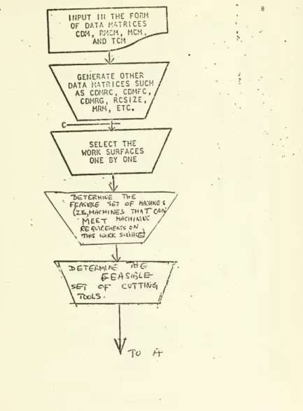
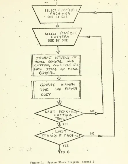
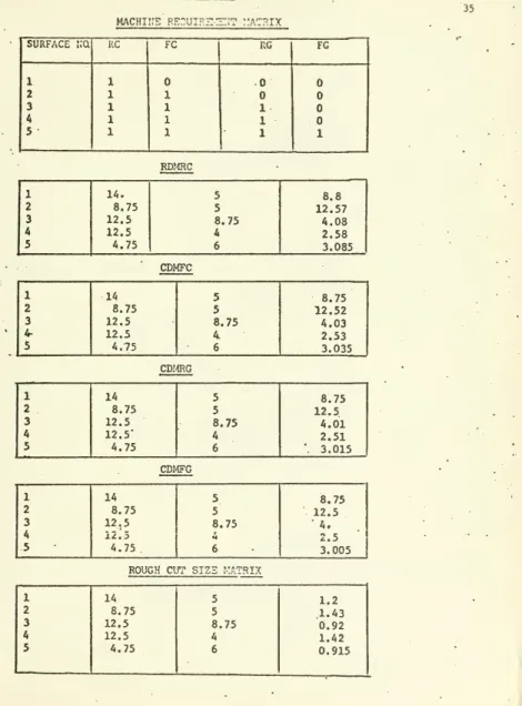
A system block diagram for the planning procedure is

given in Figure %. The following abbreviations have been used

for denoting the various data and output matrices.

CDM Component Data Matrix

CDMFC Finish Cut Component Data Matrix

CDMFG * _{Finish Grind Component Data Matrix}

CDMRC Rough Cut Component Data Matrix CDMRG Rough Grind Component Data Matrix MCM Machine Characteristics Matrix MRM Machine Rcquire^.ent Matrix

RCSIZE Rough Cut Size Matrix

RMCM RawMaterial Characteristics Matrix

INPUT Itl THE FORM OF DATA

MATRICES

MCM

31

MATRICES

AS CDHRC, CDMFC,

_/

RCSIZE

7

/

zr^ti

WORK

_/

^

\s&T

op

ATboLS.

NA

Zi

7

/

IL

hEASiSLe

CUTT^P>6

\

Corr

10

Select best

machine

and cutter

PRINT ALL

RECOM-MENDATIONS,

COR-RESPONDING,

COST & TIME

P*-TO

C

[

END

")

.

.

The input to the systcn consists of the data matrices

CDM, RMCM, MCM and TCM. The CDM describes all the specifications

of theworkpieces to be machined including all dimensions, tolerances

and surface finish grades needed. In the present systen it is

...-issuned that the machining of the part can be subdivided into the

nllling of'a number of plain surfaces and hence each row in the CDM

describes exactly one such plain surface. The RI-'CM gives a complete

description of the size, shape and the material of the blank (or raw

material). The MCM and TCM descritie the various characteristics of the

machines and tools to be considered. The specifications given .

' _{in MCM include the maaimum and minimum limits for spindle speed}

and feed rate on the machine, horsepower of the driving motor,

efficiencies of the transmission of the mach"Jnc and the driving

motor, static stiffness and the cost rates for operators, setters

and overheads. The TCM gives for each cutter, the number of teeth

on the cutter, diameter of the cutter, length of the cutting edge,

maximum force that can be resisted by the tooth tip and values

of average change tine and average regrinding tine for each cutter.

The first matrix generated by the system is the Machine

pprtulrer'enf Matrix. Thp surface finish de«?lp;natiop and th«?

tolerance specification for the three dimensions of the work surface

are considered jointly to determine the requirements of each

surface i.e., whether each of the surfaces requires some or all of

the operations; rough billing, finish milling, rough grinding and

• - . • . !

•

12

The decision on the r.achine rcqulrer.cnts is nade based on the

dimension which has the tightest tolerance specification or finest

surface finish designation. The Machine Requirements Matrix is

a pattern of I's and O's such that a '1* in the column opposite

a surface number indicates that the particular machining

operation must be performed on that surface. Appropriate machining

allowances are then added to each of the dimensions of the work

surface to generate the matrices CDMRC, CDMFC and CDMRG which describe

the siZ3 and shape of the component after the rough milling, finish

? milling and rough grinding operations respectively. The system then checks if the raw material size specified in the RMCM is

smaller or larger than that specified by the CDMRC. If it is

smaller, it prints out an errormessage and goes to the next raw

material specification. If larger, the system determines the amount

of material to be removed from the given raw material to bring it

to the size specified by CDMRC and stores it in the matrix

RCSiZE. The system repeats this process for each of the

acceptable rawmaterials. Thus, RCSIZE is actually a three dimensional

•_{'array of} numbers; each layer _{of the array corresponding}

to one

raw material. The numbers in the array are the dimensions of the

material to be removed in the milling operation for each »7ork

Surf ace. Out of all acceptable raw materials, the best is chosen by

13

The system then selects the work surfaces one at a time and determines

the set of 'feasible' machines and 'feasible' cutting tools for the

work surface picked. (By 'feasible' machines, wemean machines that

canmeet the machining requirements of the chosen work surface; the

definition of 'feasible' cutting tools is similar). Next, it chooses

combinations of feasible machines and feasible cutting tools one by

one, determines the optimum cutting conditions in each case and

selects the combination that yields the minimum optimized cost. It

then prints out the best machine, best cutter and the optimum machining

parameters for that combination along with estimates of total cost and

total time per machined piece.

The system concept suggested here is quite general and maybe

used for awide varietyof machining processes such as turning, milling,

shaping, etc. Fortunately too, the similarities in physical

character-istics of different machining processes are strong enough to permit

use of the same optimization methodology. For instance, the functional

relations between dependent variables (such as tool life and cutting

forces) and independent variables (such as machiningparameters) have

the same general form for all machining processes. Specific formulations

will indeed be needed for each type of machiningand job environment,

but the general operation andmethodologyof the systemwill be the

same

THE FACE MILLING PROCESS

Since the optimization phase requires consideration of

certain physical details of themachining process, this phase will

be illustrated for the specific case of a face milling process.

[-*

Lx

15

For the benefit of the unfamiliar reader, Figure "Ogives

averybrief description of the face millingprocess. The facemilling

cutter has its cutting teeth on the end and is rotated bymeans of

the spindle of themilling machine. Simultaneously, the work table

moves In a longitudinal direction, thus removing a thickness of

metal equal to the depth of cut given. At the end of each longitudinal

stroke, a transverse 'feed' may be given to remove an adjacent

longitudinal strip. The machining parameters of this process are

therefore the depthof cut, feed rate, cutting speed and the widthof

cut. (There are also other parameters such as the rake angle of the

teeth which havebeen left out of this illustration for simplicity.)

The cutting forces generated at the tooth tip maybe resolved into

three components, viz. the radial force P , axial force P and the

16

OPTIMIZATION METHODOLOGY

The mathematical model for optimization essentially consists

of a cost objective: function subject to a numberof constraints that

arise from the nature of thephysical process of machining. IjoJ

The total unit cost of the milling operation consistsmainly

of three parts: machining and operating costs, tool costs and

non-productive costs. The machining cost per unit Is the cost of running

themachine, cost of operator and overhead computed over the time taken

for themachiningof a single piece. The tool cost is made up of tool

setting cost, tool regrlndlng cost and tool changing cost including

cost of depreciation. Finally, the non-productive cost includes the

cost of non-cutting time forced by thenature of themachining

operationand is equal to the cost of operator labor and overhead

17 In the case of the face millinc operation, the machining

time per piece t. andthe non-cuttinc tice t. are given by

dep wid T

*-i

^-''ij "ij "ij

and

fn,

n .,

dep wid

iJ if a idle return

f-< f-i t; stroke is needed

^-^ "J-^

. ^rapid

P . otherwise

where f is the feed per tooth (inches per tooth); rapid is the feed

rate of the work table for rapid traverse in the return stroke (inches

per minute); i,J are the subscripts used to denote the i'th pass in

the depth direction and the J'th pass in the width direction; L is the length

of travel of the cutter relative to the workpiece in each longitudinal

stroke (inches); N is the number of Revolutions per minute of the

cutter; n is the number of teeth on the cutterbeing used; n ., is the

number of passes required in thewidth direction; and n^ is the dep

number of'^ccccs in the dc^th dirccticr. Tt tt""' be nctcd th—t L ''s

determined by the longitudinal dimension of the surface to be milled and

the allowance needed for the cutter approach; n, is determined by the

total thickness of material to be removed and the depth of cut given in

each pass*^ in the deoth direction;- ' and n_wid., is determined by the width''

18

width direction. The total cost of machining can be determined from

a knowledge of t-.t^ and the relevant cost rates and the number of

tool resettings and regrindings required for the machining of a

single piece. It should be mentioned that the expected number of

times the cutter is to be regrounded and reset during themachining

of a single piece is givenby E[t^/T] where T is a stochastic variable

devoting the life of the cutter (i.e., the time it can be used for

machining before failure occurs), and E[ ] stands for the expectation

operator. Empirical formulas expressing E(T) as a function of the

machining parameters are available in literature [10] and are

generally of the form E(T)" ^

—

jX^yj^z y

constants determined by the tool and work materials being used. For

thepresent purposes, we shall approximate the expected number of tool

failures (in a period of length t^^) by t,/E(T).

The total unit cost of machiningcan bewritten as:

+ (tj/I) [(C3« ^)t^^+

_(S^chg^chgl

The approximation holds very well for the case where tool failures are Poissori distributed and t^ is fairly large relative to E(T). Both of these are very reasonable assumptions for most machining situations.

X9

•where C..C-.C- are the rates for direct labor, operating overhead

and fixed overhead respectively, t ,t ,t . are respectively the

times required for initial tool setting, tool regrinding and tool

changing (including resetting) and C ^,C ,C , are the wage rates for

set gr cng tool setting, regrinding and changing.

The total unit cost of machining should be optimized with

respect to the machining parameters such as the cutting speeds, feeds,

depths andwidths of cut. However, the choice of these machining

parameters is restricted by anumber of constraints that result from

considerationof the physical process of milling and the limitation

of the available facilities. For example, the spindle speed and feed

used must liewithin the range of maximum speeds and feeds available

on themachine tool; the cutting forces should not exceed the maximum

forces that can be resisted by the work and tool holding devices; the

cuttingpower required should be less than the net power available

from the driving motor of themachine and so on. Certain restrictions

are also to be Imposed to Insure chatterless machining and to limit

theprobability of cutter failure during the machining of a single

surface to a specified maximum.

The major constraints for the case of face milling are stated 2

below. For notatlonal simplicity, the subscripts l,j (denoting the

sequential number of the pass in the depth and vd.dth directions) are

This restriction is imposed because failure of the cutter during the machining of a single workpiece is extremely inconvenient and expensive in terns of tine loss in resetting the machine and cutter in the middle of a pass.

Once again, it should be noted that the constraints may look somewhat different for other machiningprocesses, butwill be of the same general forms.

20

omitted. Except when explicitly specified, the following constraints

apply to each Individual pass.

Speed Restrictions;

where N . and N are the minimum andmaximum available spindle speed:

mln max

on the machine, respectively. There are, in addition, restrictions

on the surface speed of the cutting edge relative to the workplece.

The peripheral speed is given byV» (ttDN/12), The surface speed

constraints can then bewritten as:

12 V . 12 V

Si2.< N < ES2L

i:D ~ irD

where V is the minimum cutting speed to avoid the formation of

built up edge on the tool tip. V is themaximum cutting speed for

theprevention of excessive heating of the tool tip, and D is the

21

Feed Restrictions;

F . < fnN < F

mln - ~ max

where F . and F are theminimum andmaximum feed rates available

mln max

on the machine.

Depth of Cut Restrictions;

d < H

1 d < d

- max

where H Is the total depth of material to be removed after correcting

for finishing allowances and d Is the length of thecutting edge max

of each tooth of the cutter.

In addition, the total depth of material removed in the n.

layers should equal H. i.e..

E d.» H i-1 ^

22

Width of Cut Restrictions;

The width of cut w Is limited to aicaxlmum value w .

max Formost face millingapplications, w j^" D so that

w < D

In addition, the total widthof metal removed should equal

W, the widthof the workpiece. Hence,

r „ -W J-1 J

Force Restriction:

The maximum resultant cutting force, P , at any tool tip

must not exceed the maximum force that can be resisted by the tool tip,

P . In the case of face milling,

max

P

-res

/P^T7<

where P and P are the tangential and radial cutting forces at the

tool tip, respectively. The radial force in the case of facemilling

23

force [4,12]. The tangential cutting force is generally computed by

.empirical fomulas expressing it as a function of each of the machining

parameters. One such formula knovm as the extended cutting force law

la given byKronenberg [10] and is of the form

P^- C Af G^N^

t p 1

%ifaere k. is the modified area of the chip cross section and is given

by A."df, G is the slenderness ratio and is givenby G= d/f, and

g, h, and kare indices which depend upon the particular toolwork combination being used.

If P - C-P , the cutting force restrictionbecomes.

(^)

p I

where x-, y. and z. are indices determinedby the values of g, h, and k.

Horsepower Restriction; -, - _

The total power available at the cutter must be enough to resist

thecutting forces at the speeds being used. This requires that

P V

t-tot ^ . ,

24

where HP is the horsepower of the driving motor, P-^_^ ^ is the total

of the tangential force components with all the teeth in contact with

the workpiece, n >, is the efficiency of power transmission in the

machine, n ^ is the efficiency of the drivingmotor, and V is the mot

peripheral velocity of cutting. P^_,^

f.

assumes itsmaximum value

when all the teeth of the cutter are in contact with the work surface,

and, in this case, it is givenby

t-tot 2 ""t

Substituting this and the expression for peripheral speed V, the

power constraint

becomes-C _„ X- y- z.+l

-E^C^nd^fHl^

)<HPn.

33,000 ^24 "" / ^ •- -jjj^^^..jjj^^

Restrictions to Avoid Excessive Vibrations and Chatter;

Chatter is a function of both the cutting conditions and the

machine structure; thus it is not easy to form constraints that will

positively insure chatterless operation. Based upon experimental and

.25

Long [11], and others, the following constraint"is applied

=^-v

where n is the number of edges cutting simultaneously, X is the c

directional static stiffness of the machine frame (Ibf/in.), k^. is

theslope of cutting speed-cutting force curve, and k^ isa constant

parameter indicating the safe regionwith respect to vibrations.

(A typical value of k Is 0.2). Themaximum value ofn^ Is n/2 and

^t ^1 ^1 ^1'^ k-

_-f--

^

c d p 1

so that the chatter constraint becomes

/i/i/r^

p

Other researchers like Barash [2] suggest consideration of

the chatter problem by a constraint on the chip slenderness ratio. In

this work, the constraint used is

d/f < 50

Hopefully, these two constraints used together will keep the machining

26

Restriction of Tool Life;

It ishighly desirable that a freshly reground cutter

last for at least the time required to machinea single workpiece.

Failure of the cutting tool in the middle of machining is extremely

Inconvenient and expensive in terms of time lost in resetting the

machineand cutter in the middle of a pass. However, since tool

failure is inherently probabilistic in nature, this constraint can

never be satisfied with absolute certainty. Hence, it is converted to

a *chance constraint' of the form

PrfT> tj^} 2 a.

wherea is chosen depending on the degree of assurance with which the

tool life constraint is desired to be satisfied. It is obviously

in-convenient to handle the tool life constraint in its probabilistic form

directly. If the probability distribution of the tool life is known,

the constraint can be transformed into a more convenient formby

using the properties of the distribution. The foregoing inequality can

berewritten as

27

vhere E(T) and a_ are themean and standard deviation of the tool life

respectively. Let K be <

whichT belongs such that

respectively. Let K be a constant defined for the distribution to

Pr{e > K }- a a

where e is the standardizedvariate of the distribution. Using this

notation,

Pr{i^-Effl->K

_.>»

life constraint can thus be expressed as

t, - E(T)

o^

-^«

T

Substituting for t- and transforming,

^dep'^wid L C'

TV

\'T

Very little experimental work has been done to establish the natureof

the probability distribution of tool life. It is known, however [21],

.28

carbide tools, failure due to excess flank wear, and failure due to

chipping. It can be expected that the probability distributions of

life of the tool would be different for the two different modes of

failure. The Poisson distributionhas been suggested for tool

failures bychipping [1] and some form of modified normal distribution

for the tool failure by flankwear. The actual distribution of tool

lifewould, therefore, be the composite distribution obtained by

taking theweighted mean of the distributions in the case of the two

different modes of failure, welghtages being assigned on thebasis of

relative dominance of eachmode of failure. Moreover, the failure of

amilling cutter is governed by the failure of any one of its teeth

and so the appropriate distribution is the distribution of the minimum

of the lives of the individual teethof the cutter. Therefore, the

probability distribution of the life of a cutter has beenderived from

that of an Individual toothwhich in turn is obtained from the

distributions of failures by chipping and failures by flank wear. With

the distribution of T known, one can easily read off the value of K

29

FINAL FORM OF THE OPTIMIZATION MODEL

The optimization problem as stated above is quite a formidable

one, one withnon-linear objective function and many non-linear constraints.

By a detailed consideration of the natureof the objective function, nature

of the constraints and the physical process of milling the reasonable

modifications and simplifications of the above mathematical mod^lhave

been made. It is also found convenient to define the transformedvariables

V

Expressed in terms of those transformed variables, the above

mathematical model can be shown to reduce to a convex objective function

with a set of linear constraints. It reduces to the form

„, , , , *=10^1lV^12'^2-'^13^3 ^ «=20-^2lV*=22'^2+'^23'^3

nlnlnlze Z" e + e

subject to a number of constraints

ax

where the b. s and c.. s are functions of the constants and parameters of

3D

The technique of optinlzatlon employed is a version of the

gradient projection method very similar to that suggested by Rosen [17],

This method belongs to the general class of 'hill-climbing' methods

for optimization of non-linear functions. It always attempts to travel

In the locally steepest direction of ascent (or descent) while not

allowing the point to leave the constrained set. The optimum size of

the step is then determined. Once the optimum Is found on the line

of steepest ascent, anew gradient evaluation is carried out and the

procedure repeats itself until a point sufficiently close to the global

optimum is reached.

Notice that theobjective function we are encountered with is

very smooth, convex and 'well-behaved' and satisfies all. the regularity

conditions needed for convergence. It is-therefore reasonable to

expect the procedure to converge in a relatively small number of

iterations. Moreover, theobjective function is composed of the sum

of two exponential terms which makes it extremely easy to analytically

compute the gradient vector at any stage of the iterative procedure.

It is precisely these features that make the gradient methods so

convenient for this class of problems.

The optimization procedure is carriedout by means of the

computer program OPTIMIZEwhich is part of the software that comprises

the planning and optimization system.

This is by nomeans an accident; nor is it peculiar to the face milling process. It can be shown that the model will reduce to a similar form for most machining processes.

AN ILLlI3TRATT0:i OF USE OF THE SYSTE:-! ₃₁

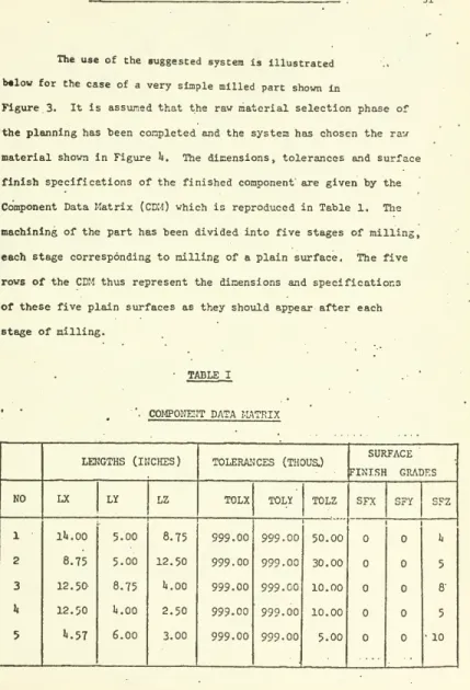
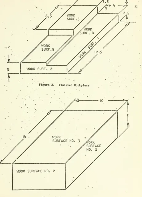
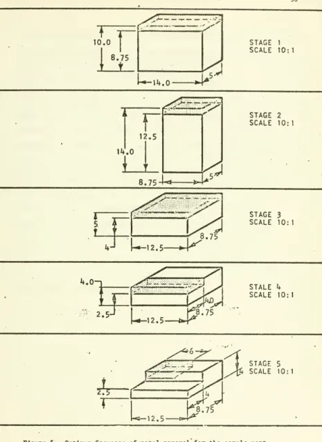
The useof the _{suggested system is illustrated} !.

b«lowfor the caseof a very _{simple milled part shown in}

Figure 3. It is asstimed that the rawmaterial selection phase of

the planninghas been conpletedajid the system has chosen the rav

material shovn in Figure h. The dimensions, tolerances and surface

finish specifications of the finished component'are given by the

Component DataiMatrix (CDM) which is reproducedin Table 1. The

machining of the part has been divided into five stages of milling,

each stage corresponding to milling of a plain surface. The five

rows ofthe CDM thus represent the dimensions and specifications

of these five plain surfaces as they should appear after each

stage of milling.

TABLE I

Plgurc 3. . Finished Workpiece

33

The. dincnclonc of the raw natarial for each stage of

milling are given by the Raw Material CharacterisCics Matri:: (KMCM)

shown In Table II.

•_{TABLE II}

. .

RAW MATERIAL CHARACTERISTICS

MTRIX

In the case of the Tool Characteristics Matrix, the coliu?.ns read respectively, cutter number, nur.ber of teeth, diameter of the cutter,.

length of the cutting edge, naxir.iun force that can be resisted by

the tooth tip, tine for regrinding and tin-.e for changing the cutter. 34

TABLE III

f4AC}{INE CHAR.'VCTKRISTICS MATRIX

NO. NMIN NMAX FMIN FMAX HP EFFYl JJ'FY2 LA>II5DA CI C2 C3 TSI

30.0 AO.O 800.0 500.0 0.2 0.3 5.0 3.0 20.0 15.0 0.7 0.7 1.0 0.9 210000.0 1]0000.0 0'.2 0.3 0.2 0.2 1.1 20. 0.1 AO.

TOOL CHAR/\CTERISTICS Il.^TRIX

TABLE IV

machii:e'reouipz:z:jt ^ix SURFACE i;a

STAGE 1 SCALE 10:1 8,75 STAGE 2 SCALE 10:1

cp

Ui

^xO^^^.-^

7^

<

^.75

37

The progran CALCULATE then uses the "data generated by MODIFY

to calculate the values of the various coefficients and constants

In the constraint matrix and the objective function. The

program CHOOSE considers all the available machine-cutter

combinations (4 in this case) one after the other and uses the

programs MODIFY, CALCULATE and OPTIMIZE to determine tlie optimum

conditions for each combination. It then chooses the best

combination of machine and cutter and the corresponding optimized

machining parameters. These results^, along with the nuriber

of passes required in the depth and width directions and estimates

of total machining time and machining cost per piece are printed

out by the system. For purpose ofmaking comparisons and any

necessary compromises, the optimized costs of machining with all

other possible machine-cutter combinations also are printed out

*_as supplementary data. The reconunendations of the machines,

cutters and machining parameters for each of the five work surfaces

TABLE V

RECo:rinr:D MAC!iT:;ns, cutters ,v:n yu.\cHTNiNr. parameters

38

39

other criteria such as maximum production rate [1] maximum profit [13],

minimum time [3], etc. Similarly, while working on automatics

employing several tools simultaneously, fixed tool servicing schedules

might bepreferable to changing the individual tools when failure is

expected.

The authors believe that systems for automated manufacturing

planning such as the one suggested in this article are likely to find

wide practical utility in the near future. Manufacturing systems are

typically complex and extremely djmamic. Development of such '

self-optlmizing' units should prove to be amajor technological advance for

•40

refere:,'ces

1. Armerago, E.J. A., and Russell, J.K., "Maximum Production Rate as a Criterion for the Selection of Machining Conditions", International Journal of Production Research, Vol. 16, pp. 15-23, 1966.

2. Batra, J.L., and Barash, M.M., "Computer-Aided Planning of Optimal Machining Operations for Multi-Tool Set-ups with Probabilistic Tool Life", Report No. 49, Purdue Laboratory forApplied Industrial Control, Lafayette, Indiana, January 1972.

3. Berra, P.B., and Barash, M.M., "Automated Process Planning and

Optimization for a Turning Operation", International Journal of Production Research, V. 7, No. 2, pp. 93-103, 1968.

4. Berra, P.B., and Barash, M.M., "Investigation of Automated Planning and Optimization of Metal Working Processes," Report No. 14, PurdueLaboratory for Applied Industrial Control, Lafayette, Indiana, July 1968.

5. Brewer, R.C.,and Reuda, R., "A Simplified Approach to Optimum Machining", Engineer's Digest. V. 24, No. 9, pp. 133-151, September 9, 1963.

6. Challa, Krishna "An Investigation into the Automated Planning and Optimization of the Milling Process", Unpublished

Master's Thesis, Syracuse University, Syracuse, NewYork, 1971.

7. Cincinnati Milling Machine Company, "_{A Treatise} on Milling and MillingMachines", 1948.

8. Colding, B.N., "A Three Dimensional Tool Life Equation - Machining Economics", Journal of Engineering for Industry (Trans, of ASME), pp. 239-249, August 1959.

9. Gilbert, W.W., "Economics of Machining", Chapter in Machining Theory

4;

10. Kronenberg, M., "Machining Science and Application", Permagon

Press, NewYork, 1966.

11. Lemon, J.R., and Long, G.W., "Survey of ChatterResearch at Cincinnati Milling Machine Company", International Journal of MachineTool Design and Research, 1966, pp. 5A5-586.

12. Maslov, P., Danllevsky, V., and Sasov, V., "_{Engineering Manufacturing}

Processes, Foreign Languages, PublishingHouse, Moscow, USSR,

1963.

13. Okushlma, K., and Hltomi, K., "A Study of Economical Machining

(AnAnalysis of Maximum Profit Cutting Speed)", Memoirs of Kyoto University, V^ 25, pp. 377-383, October 4, 1963.

14. Opltz, H., and Simon, W., "EXAPT 1 and EXAPT 2 Part Programmer

Reference Manuals", EXAPT -Association, 51 Aachen, P.O. Box 587,

Germany.

15. Peters, F.A., "Computer Assistance In Programming for Numerical

Control", Machinery and Production Engineering (London), V. 108, pp. 572, March 16, 1966.

16. Rlchter, G., and Frankfurt, L.B., "Design and Practical Application

of theAUTOPIT System", MachineTool Engineering and ProductionNews, English translation from Werkstatt und

Betrleb (German), V. 99, pp. 98-104, April 1966.

17. Rosen, J.B., "The Gradient Projection Method for Non-linear Programming; Part I", Journal of the Society of Industrial Mathematics. V. 8, No. 1, pp. 181-217, March 1960.

18. Scott, R.B., "Regenerative Shop Planning", SpecialReport No. 586, American Machinist, pp. 89-94, March 28, 1966.

19. Spur, G., "Automatic Programming of Numerically Controlled Lathes", Proceedings of the International Machine Tool Design and Research Society. September 25-28, 1967.

20. Taylor, F.W., Proceedings of Institutionof Engineers (London)

pp. 258-289, 1946.

21. Taylor, J., "Carbide Tool Variance and Breakage -Unknown factors InMachining Economics", Proceedings of International Machine Tool Design and Research Society, 1967, pp. 487-504.

42

22. Tobias, S.A.."Machine Tool Vibration," Wiley, 1965.

23. Tobias, S.A., and Sadek, M.M., Personal Conmunication, dated

August 5, 1969.

24. Wagner, J.G., and Barash, M.M., "The Nature of the Distribution

of Life of High Speed Steel Tools and the Significance inManufacturing", ResearchMemorandumNo. 69-2, School of Industrial Engineering, PurdueUniversity, Lafayette, Indiana, May 1969.

25. Weill, R., "Optimizing Machining Conditions in Numerical and Adaptive Control", Proceedings of the 7th International Conference on Manufacturing Technology, Ann Arbor,

pp. 569-580.

26. I.B.M., "Automated Manufacturing Planning," Manual No. E20-0146-0, I.B.M. Technical Publications. NewYork, 1967.