Comparing Optimal Relocation Operations With Simulated Relocation Policies in One-Way Carsharing Systems

(1)

Relocation Policies in One-Way Carsharing Systems

The MIT Faculty has made this article openly available.

Please share

how this access benefits you. Your story matters.

Citation

Jorge, Diana et al. “Comparing Optimal Relocation Operations With

Simulated Relocation Policies in One-Way Carsharing Systems.”

IEEE Transactions on Intelligent Transportation Systems 15,

4 (August 2014): 1667–1675 © 2014 Institute of Electrical and

Electronics Engineers (IEEE)

As Published

http://dx.doi.org/10.1109/TITS.2014.2304358

Publisher

Institute of Electrical and Electronics Engineers (IEEE)

Version

Author's final manuscript

Citable link

http://hdl.handle.net/1721.1/112401

Terms of Use

Creative Commons Attribution-Noncommercial-Share Alike

(2)

Comparing optimal relocation operations with

simulated relocation policies in one-way

carsharing systems

Diana Jorge, Gon�alo Correia, and Cynthia Barnhart

Abstract-One-way carsharing systems allow travelers to pick up a car at one station and return it to a different station, thereby causing vehicle imbalances across the stations. In this paper, realistic ways to mitigate that imbalance by relocating vehicles are discussed. Also presented are a new mathematical model to optimize relocation operations that maximize the profitability of the carsharing service and a simulation model to study different real-time relocation policies. Both methods were applied to networks of stations in Lisbon Portugal. Results show that real time relocation policies, and these policies when combined with optimization techniques, can produce significant increases in profit. In the case where the carsharing system provides maximum coverage of the city area, imbalances in the network resulted in an operating loss of 1160 €/day when no relocation operations were performed. When relocation policies were applied, however, the simulation results indicate that profits of 854 €/day could be achieved, even with increased costs due to relocations. This improvement was achieved through reductions in the number of vehicles needed to satisfy demand and the number of parking spaces needed at stations. This is a key result that demonstrates the importance of relocation operations for sustainably providing a more comprehensive network of stations in one-way carsharing systems, thus reaching a higher number of users in a city.

Index

Terms-Mathematical programming, one-way carsharing, relocation operations, simulation.

I. INTRODUCTION

T

HROUGH the last decades, changes have occurred in urban transport. Despite greater accessibility provided by private transport, the result has been increases in levels of congestion, pollution, and non-productive time for travelers, particularly in peak hours [ 1]. There are also opportunity costs associated with using urban land for parking spaces instead of other more productive activities. In America, for example, automobiles spend around 90% of their time parked [2]. These issues are mitigated by ·public transport, but it has other disadvantages, for example, poor service coverage, schedule inflexibility and lack of personalization. In addition, providing public transport for peak hour demand can result in idle vehicles for much of the day, resulting in inefficiencies and high cost of service.

Strategies are needed to address these issues and simultaneously provide people the mobility they need and desire. One strategy considered is that of carsharing. Carsharing systems involve a small to medium fleet of

vehicles, available at several stations, to be used by a relatively large group of members [3].

The origins of carsharing can be traced back to 1948, when a cooperative known as

Se/age

initiated services in Zurich,

Switzerland. In the US, carsharing programs only appeared later in the 1980s, within the

Mobility Enterprise

program [3].

In Asian countries, such as Japan and Singapore, these systems appeared more recently.

Carsharing has been observed to have a positive impact on urban mobility, mainly by using each car more efficiently [4], [5]. The use of carsharing systems generally leads to a fall in car ownership rates and thus to lower car use, according to Celsor and Millard-Ball [6]. More recently, Schure et al. [7] conducted a survey in 13 buildings in downtown San Francisco and concluded that the average vehicle ownership for households that use carsharing systems is 0.47 vehicles/household compared to 1.22 vehicles/household for households that do not use carsharing systems. Moreover, a study by Sioui et al. [8] surveyed the users of

Communauto,

a

Montreal carsharing company, and concluded that a person who does not own a vehicle and uses carsharing systems frequently (more than 1.5 times per week) never reaches the car-use level of a person who owns a vehicle: there was a 30% difference between them. This idea is reinforced by Martin and Shaheen [9] who concluded through a survey in US and Canada that the average observed vehicle-kilometers traveled (VKT) of respondents before joining carsharing was 6468 km/year, while the average observed VKT after joining carsharing was 4729 km/year, which constitutes a decrease of 27% (1749 km/year).

Furthermore, some recent studies concluded that carsharing systems also have positive environmental effects. For instance, Martin and Shaheen [9] noted from the VKT estimations presented before that greenhouse gas (GHG) emissions of the major carsharing organizations in the US and Canada can be reduced by -0.84 t GHQ/year/household. While most members increase their emissions; there are compensatingly larger reductions for other members who decrease their emissions. Moreover, Fimkom and MUiier [10], through a survey of a German carsharing company, concluded that the CO2 emissions are decreased between 312 to 146 Kg CO2/year per average carsharing system user.

(3)

divided into round-trip (two-way) systems and one-way systems. Round-trip carsharing systems require users to return the cars to the same station from where they departed. This simplifies the task of the operators because they can plan vehicle inventories based on the demand for each station. It is, however, less convenient for the users because they have to pay for the time that vehicles are parked. In one-way carsharing systems, users can pick up a car in a station and leave it at a different one [11]. In theory, therefore, one-way carsharing systems are better suited for more trips than round trip services that typically are used for leisure, shopping and sporadic trips - short trips in which vehicles are parked a short duration [12]. This statement is supported by various studies, including that by Costain et al. [13], who studied the behavior of a round-trip carsharing company in Toronto, Canada and concluded that trips are mostly related to grocery or other household shopping purposes. A study performed in Greece by Efthymiou et al. [14] also concluded that the flexibility to return the vehicle to a different station from the one where it was picked up is a critical factor in the decision to join a carsharing service. However, one-way carsharing systems present an operational problem of imbalances in vehicle inventories, or stocks, across the network of stations due to non-uniformity of trip demand between stations. Despite this, a great effort has been made to provide these flexible systems to users in the last years.

Previous research has proposed several approaches to solve this problem, such as: vehicle relocations in order to replenish vehicle stocks where they are needed [15], [16], [17], [18], [19], [20]; pricing incentive policies for the users to relocate the vehicles themselves [21], [22]; operating strategies designed around accepting or refusing a trip based on its impact on vehicle stock balance [23], [24]; and station location selection to achieve a more favorable distribution of vehicles [24]. Correia and Antunes [24] proposed a mixed integer programming model to locate one-way carsharing stations to maximize the profit of a carsharing company, considering the revenues (price paid by the clients) and costs (vehicle maintenance, vehicle depreciation, and maintenance of parking spaces), and assuming that all demand between existing stations must be satisfied. In applying their model to a case study in Lisbon, Portugal, tractability issues resulted and the model was only solvable with time discretization of I 0-minute steps. The model did not allow integrating relocation operations due to the complexity already reached with the location problem.

In this paper, the same case study as the one in [24] is considered and station location outputs are generated using their model, but now with time discretization of I -minute. When a IO minute based model is used, all of the travel times between stations are rounded to the next multiple of 10. So, users are paying for minutes that they are not really using vehicles. Moreover, the vehicles are also considered available only in each multiple of IO minutes, while the reality is that they could be available earlier. Therefore, a 1 minute based model is always more realistic than a 10 minute based model or a model that considers larger time steps.

A new model is presented to optimize relocation operations on a minute-by-minute basis, given those outputs for station locations brought from the previously referred model. Thus, the two problems, station locations and relocation operations, will not be considered at the same time. The objective function is the same, profit maximization, but in the relocat!ons model, a cost for the relocation operations is also added. The vehicle relocation solutions generated with this approach are later compared to those obtained with a simulation model built to evaluate different real-time vehicle relocation policies. With this comparison, the impacts of relocation operations on the profitability of one-way carsharing systems are then analyzed, and insights into how to design and implement real-time rebalancing systems are gained.

The paper is structured as follows. In the next section, a new mathematical model is presented to optimize relocation operations, given an existing network of one-way carsharing stations. Then, a simulation model and a specification of several real-time relocation policies are presented. In the following section the case study used for testing the relocation methodologies is described, as well as the data needed and the main results reached. The paper ends with the main conclusions extracted from the paper.

II. MATHEMATICAL MODEL

The objective of the mathematical programming model presented in this section is to optimize vehicle relocation operations between a given network of stations (using a staff of drivers) in order to maximize the profit of a one-way carsharing company. In this model, all demand between existing stations is assumed to be satisfied. The notation used to formulate the model (sets, decision variables, auxiliary variable, and parameters) is the following:

Sets:

N

=

{1, ... , i ... N}: set of stations;

T

=

{1, ... , t ... T}: set of minutes in the operation period; X

=

{11, ... , it-t, it, it+t, ... , NT}: where it represents

station i at minute t: set of the nodes of a time-space network combining the N stations with the T minutes;

A1

= { ... , (

it, it+6

b) , ... } ,

it E X: set of arcs over which vehicles move between stations i and j, \fi, j E N, i

*

j, between minute t and t + 6fj, where 6fj is the travel time (in number of minutes) between stations i and j when the trip starts at minute t;

A2 ={ ... ,Cit, it+1), ... }, it EX: set of arcs that represent vehicles stocked in station i, \fi EN, from minute t to minute

t

+

1.

Decision variables:

R1d t : number of vehicles relocated from i to j from

t+Bij

minute t tot+ 6fJ, \f (it, jt+6

f

_i

)

E A1;

Z1: size of station i, \fi E N, where size refers to the number of parking spaces;

(4)

a

1t

: number of available vehicles at station i at the start of a

1t

e N

°

\fi

t

e X

minute

t,

\fi

t

EX.

(7)

(8)

Auxiliary variables:

S

itit

+i: number of vehicles stocked at each station i from

minute t to t

+

1, V{i

t

, i

t

+

1)

e A

2

, this is a dependent variable

only used for performance analysis.

Parameters:

D

1t

l

_{t+S j}

_f

: number of customer trips (not including vehicle

relocation trips) from station i to station j from t to t

+

c5f1, \f (i

t

, it+6f1) E A1;

P: carsharing fee per minute driven;

Cmv: cost of maintenance per vehicle per minute driven;

c5f1: travel time, in minutes, between stations i and j when

departure time is t, \fi

t

E X, j E N;

Cmp: cost of maintaining one parking space per day;

Cv: cost of depreciation per vehicle per day;

Cr: cost of relocation and maintenance per vehicle per

minute driven.

Using the notation above, the mathematical model can be

formulated as follows:

(1)

subject to,

The objective function (I) is to maximize total daily profit

(n) of the one-way carsharing service, taking into

consideration the revenues obtained through the trips paid by

customers, relocation costs, vehicle maintenance costs, vehicle

depreciation costs, and station maintenance costs. Constraints

(2) ensure the conservation of vehicle flows at each node of

the time-space network, and Constraints (3) compute the

number of vehicles at each station i at the start of time

t,

assuming that vehicles destined to i at time

t

arrive before

vehicles originating from i at time t depart. Constraints ( 4)

guarantee that the size of the station at location i is greater

than the number of vehicles present there at each minute t. In

practice, size will not be greater than the largest value of a1

t

during the period of operation otherwise the objective function

would not be optimized. Expressions

(5)-(8)

set that the

variables must be integer and positive.

III. SIMULATION MODEL

In order to test real-time relocation policies, a discrete-event

time-driven simulation model has been built using AnyLogic

(xj technologies), which is a simulation environment based on

the Java programming language. It is assumed that a trip will

be performed only if there is simultaneously a station near the

origin of the trip and a station near the trip's destination. The

effects of congestion on the road network are captured with

different link travel times throughout the day.

In each minute, trips and relocation operations are triggered

and the model updates a number of system attributes,

including: number of completed minutes driven by customers

and by vehicle relocation staff; vehicle availability at each

station; total number of vehicles needed; and maximum

vehicle stock (that is, number of parked vehicles) at each

station, which is used to compute the needed capacity of each

station. These updated values are used to compute the

objective function. It includes all revenues (price rate paid by

customers) and costs (vehicle maintenance, vehicle

depreciation, parking space maintenance, and relocation

operations). To satisfy all demand, a vehicle is created (the

fleet size is correspondingly increased) each time a vehicle is

needed in a given station for a trip and there are no vehicles

available. Thus the fleet size is an output of the simulation.

The period of simulation is between 6 a.m. and midnight

which is the same period used in (24]. At the end of the

simulation run, it is possible to obtain the total profit and the

total number of parking spaces needed in each station.

A. Relocation Policies

Two real-time relocation policies (1.0 and 2.0) were tested

in the simulation. For each one, it is determined for each

minute of the day at each station s if the status of s is that of

supplier (with an excess number of vehicles) or demander

(with a shortage of vehicles). For policy 1.0, a stations at time

(5)

t is classified as a supplier if, on a previous day of operations,

the average number of customer trips destined for that station

at instant t + x exceeds or equals the average number of

customer trips that depart that station at the same period. Note

that only customer trips, and not repositioning trips, are

included in this calculation. Each station that is not designated

as a supplier is classified as a demander. In this policy, x is

varied between

5 and 20 minutes in

5 minutes increments to

determine the supplier and the demander stations. If s is

classified as a supplier, its supply is equal to the number of

extra vehicles (those not needed for serving customer demand)

at s at time t, multiplied by a relocation percentage that is a

parameter. Ifs is classified as a demander, its demand for

vehicles is set equal to the number of additional vehicles

needed to serve demand at time t + x. For relocation policy

2.0, the process is the same, but .x is set equal to 1 minute to

determine the set of supplier stations and the associated

supplies are determined as described for policy 1.0. The

demander stations and their demand are determined as in

relocation policy 1.0.

A schematic representation of these policies is shown in

Fig. I.

Fig. 1 Policies 1.0 and 2.0 schematic representation

For each time t, given these calculated values of vehicle

supply or demand at each station, the relocation of vehicles

between stations is determined by solving a classic

transportation problem. The objective is to find the minimum

cost distribution of vehicles from m origin nodes (representing

supplier stations) to n destination nodes (representing

demander stations), with costs equal to total travel time. An

artificial supply node and an artificial demand node are added

to the network, with all supply and demand concentrated at the

respective artificial nodes. The artificial supply node is

connected to the supply nodes, which are linked to the demand

nodes, and finally the demand nodes are linked to the artificial

demand node (as shown Fig. 2). For each arc, the following

three parameters are defined: cost of the arc (travel time);

lower bound on arc flow (minimum number of vehicles); and

upper bound on arc flow (maximum number of vehicles). On

each arc from the artificial supply node to a supply node i, the

lower and upper bounds on flow equal the supply at i and

travel time on the arc is 0. For each arc between a supply node

at station i and a demand node j, the lower bound on flow is

zero and the upper bound is the minimum of the supply of

vehicles at i and the number of vehicles demanded at j. On

each arc between a demand node j and the artificial demand

node, the lower and upper flow bounds equal the demand at j

and travel time on the arc is 0. When there is imbalance

between total supply and total demand either, one extra supply

node or one extra demand node is created.

In the simulation, an optimal relocation is determined using

a minimum cost network flow algorithm that is available in

the simulation programming language Java [25].

Fig. 2 Minimum cost flow algorithm scheme

As it is referred above, for each simulation run, two tuning

parameters, the relocation percentage and x, are defined. The

relocation percentage multiplied by the supply (of vehicles) at

a supplier station represents the value of the supply input to

the transportation algorithm. x represents the time period used

for the minute-by-minute calculation for each station to

determine its status as either a supplier or demander of

vehicles.

Using relocation policies 1.0 and 2.0 as a starting point,

three variants of these two policies were developed for each of

them. The first is that each supplier station is required to keep

at least one vehicle at that station at all time steps, that is, its

supply is equal to the number of extra vehicles minus I at time

t, multiplied by the relocation percentage (policies I .A and

2.A). The second is that the distribution of vehicles at each

station at the start of the day is set to that generated by the

mathematical model defined in the previous section (policies

l .B and 2.8). And the third is the same as the second with

priority given to stations with the greatest demand for vehicles

(policies l .C and 2.C). In practice this is done through

reducing artificially the travel time to those stations that need

a higher number of vehicles, thus making them more attractive

as a destination for the vehicles according to the assignment

method explained before. Travel times to a demander station

are reduced as a function of the relative magnitude of demand

at that station. For example, if demand at station s equals or

exceeds 10% of the total demand for vehicles at all demander

stations, travel times between supplier stations and station s

are decreased by 10% (which is done by multiplying travel

times by 0.9).

A schematic representation of the methodology that is used

in this paper is presented in Fig. 3.

Fig. 3 Schematic representation of the methodology used

IV. LISBON CASE STUDY

The case study used in this paper is the same as in [24]. It is

the municipality of Lisbon, the capital city of Portugal. Lisbon

has been facing several mobility problems, such as traffic

congestion and parking shortages due to the increase in car

ownership and the proliferation of urban expansion areas in

the periphery not served by public transport. Moreover, public

transport, even with the improvements that have been

achieved, was not able to restrain the growth in the use of

private transportation for commuter trips. For these reasons,

the municipality of Lisbon is a good example where different

alternative transportation modes, such as carsharing, may be

implemented.

A. Data

The data needed are the following: a carsharing trip matrix,

a set of candidate sites for locating stations, driving travel

(6)

times, and costs of operating the system. The trip matrix was obtained through a geo-coded survey conducted in the mid-1990s and updated in 2004 in the Lisbon Metropolitan Area (LMA). The survey data contains very detailed information on the mobility patterns of LMA, including origins and destinations, time of the day and transport mode used for each trip. This survey was filtered through some criteria, such as age of the travelers, trip time, trip distance, time of the day in which the trip is performed, and transport mode used, in order to consider only the trips that can be served by this system, resulting in 1777 trips. The candidate station locations were defined by considering a grid of squared cens (with sides of length 1000m) over Lisbon, and associating one location with the center of each cell. The result was a total of 75 possible station locations. This is obviously a simplification. To implement a carsharing system in a city, a detailed study of appropriate locations would be necessary. Travel times were computed using the transportation modeling software VISUM (PTV), considering the Lisbon network and the mobiJity survey referred above, and were expressed in minutes. The carsharing system is available 18 hours per day, between 6:00 a.m. and 12:00 a.m. The morning and afternoon peaks correspond to the periods between 8:00 a.m. and 10 a.m. and 6:00 p.m. and 8 p.m., respectively. To compute the costs related to the vehicles, it is considered an "average" car, whose initial cost is 20000€, and that this car is mainly driven in a city. The costs of running the system were calculated as realistic as possible:

Cm1 (cost of maintaining a vehicle): 0.007 euros per minute. This cost was calculated using a tool available on the internet that was developed by a German company, INTERFILE [26], and includes insurance, fees and taxes, fuel, maintenance and wear of the vehicle;

Cv (cost of depreciation per vehicle): 17 euros per day, calculated using the same tool referred above [26] and considering that the vehicles are used during 3 years. It was also considered that the company needed funy financing for the purchase of the vehicles with an interest rate of 12% and vehicles' residual value equal to 5000€;

Cr (cost of relocating a vehicle): 0.2 euros per minute, since the average hourly wage in Portugal is 12 euros per hour;

Cm2 (cost of maintaining a parking space): 2 euros per day, this cost is smaner than the parking fee in a low price area in Lisbon, considering that the city authorities would be able to give support to these types of initiatives.

The carsharing price per minute, P, was considered to be 0.3 euros per minute, which is based on the rates of

car2go

[27].

The station location model [24) was run for three scenarios, with a minute-by-minute discretization of time (note that this model does not include vehicle relocations). The three

networks used in this work are the three found in [24], as wen as the trip matrix used. In the first, the number of stations was constrained to be just 10 (considered a sman network). In the second scenario, the stations were freely located to maximize profit (any number, any location). In the third scenario, stations were located to satisfy an demand in the city (where there is demand, there is a station). The results, including station locations, number of stations, and associated profits, are presented in Fig. 4.

Fig. 4 Location model solutions

B. Results

The optimum relocation operations were determined using model (I )-(8), and an relocation policies were simulated with an possible parameters' combinations, for each of the three station location solutions (scenarios) generated with the approach of [24]. The value of x was varied between

5

and 20

minutes in

5

minutes increments, as it is referred in Chapter III. This range was selected because most travel times are between these two values. The relocation percentage was varied between 0% (no relocations) and 100% (an available vehicles in the supplier stations can be relocated) in 10% increments. For policies l .C and 2.C, simulation results were generated for the fonowing combinations of parameters: 0.1/0.9 (more that 10% of demand in a station, 90% decreasing of travel time), 0.3/0.7, 0.5/0.5, 0.7/0.3, and 0.9/0.1. In the end, the number of simulation runs was 1920.

For an the scenarios, the mathematical model was run in an i7 processor @ 3.40 GHz, 16 Gb RAM computer under a Windows 7 64 bit operation system using Xpress, an optimization tool that uses branch-and-cut algorithms for solving MIP problems [28]. The solutions found were always optimal. Xpress took about 206min to reach the optimal solution for s_cenario 1, 5min for scenario 2, and 8.3s for scenario 3. The time that the model took to run is reasonable even for the bigger scenario with 69 stations located. The factor that influences how quickly the solutions are achieved is the number of stations doubtless.

With respect to the simulation model, there was the need to run it many more times than the optimization routine, but each time the model took only few seconds to run.

In Table I, the best simulation results for each relocation policy are shown.

TABLEI Station network

(scenarios) Indicators

Results for the Different Relocation Policies Optimization of the station

(7)

x (min) 5 JO 15 5 IO JO JO JO

Best relocation % 50 90 100 60 80 100 40 90

Vehicles 390 264 273 262 264 257 267 318 222

Parking spaces 739 533 490 550 412 409 480 415 334

69 (full demand Time driven (min) 23711 23711 23711 23711 23711 23711 23711 23711 23711 attended) Time of relocations _(min) 0 4008 2921 4800 4346 5169 2967 2661 9051

Demand _0.7/0.3 -proportion/Travel _0.9/0.I 0.1/0.9 time decreasing Profit (€/da�} -1160.7 591.7 742.1 433.3 766.1 726.5 854.9 179.1 695.1 x (min) 5 5 5 5 15 5 5 5 Best relocation % 0 0 10 0 10 0 0 0 Vehicles 121 121 121 121 126 125 121 126 126 Parking spaces 241 241 241 240 195 195 241 195 195

34 (free Time driven (min) 10392 10392 10392 10392 10392 10392 J0392 J0392 10392

optimum) Time of relocations _(min) 0 0 0 4 0 54 0 0 0

Demand

0.1/0.9-proportion/Travel _0.3/0.7 all equal

time decreasing Profit (€/da�} 505.9 505.9 505.9 507.1 512.9{·} 519.1{ .. } 505.9 512.9{·} 512.9(•} x (min) 5 5 5 5 5 5 5 5 Best relocation % 0 0 0 0 0 0 0 0 Vehicles 22 22 22 22 22 22 22 22 22 Parking spaces 42 42 42 42 29 29 42 29 29

Time driven (min) 2125 2125 2125 2125 2125 2125 2125 2125 2125

10 (small network) Time of relocations ₀ ₀ ₀ ₀ ₀ ₀ ₀ ₀ ₀

(min) Demand

proportion/Travel all equal all equal

time decreasing

Objective {€/da�} 164.6 164.6 164.6 164.6 190.W} 190.W} 164.6 190.�·} 190.6{*} (*) no relocations occur, profit achieved only by bringing the initial availability from optimization

( .. ) this profit is achieved using relocations and bringing the initial availability from optimization

Analyzing Table J and comparing to the solution with no relocations, policy 1.0, achieves better results only for the 69 station scenario, increasing from -1160.7€/day (losses) to 591.7€/day (profit). This profit is achieved by setting the x parameter equal to

5

minutes and the relocation percentage equal to 50%. Similar results to policy 1.0 are evident for policy 2.0, but policy 2.0 achieves a greater profit (742.1€/day), with the relocation percentage set to 90%, and x equal to 10 minutes.

Policy I .A achieves better results (a profit of 433.3€/day) when compared to the solution with no relocations only for the 69 station scenario, using a relocation percentage equal to 100% and x equal to 15 minutes. This profit, however, is lower than the profits reached by using policies 1.0 and 2.0.

For policy 1.8, it is possible to improve profits for all scenarios compared to the model with no relocations; however, for the 34 station and 10 station scenarios, profit increases are achieved by using the initial availability of vehicles at each station brought from model (1 )-(8). Profit is 766.1€/day for the 69 station scenario, using a relocation percentage equal to 60% and an x equal to

5

minutes. For the scenarios with 34 stations and 10 stations, however, the increase in profit is very low.

With respect to policy l .C, results are better than the no relocation solution for the 69 station scenario. The best result, 726.5€/day, is achieved for two fraction-of-demand, fraction of travel time scenarios, (0.7/0.3) and (0.9/0.1), a relocation percentage equal to 80%, and x equal to 10 minutes. For the

34 station scenario, the profit is 519.1€/day, which is similar to that obtained with no relocations (512.9€/day).

For policy 2.A, results are similar to those for policy I .A, but with greater profit (854.9€/day), using a relocation percentage equal to 100% and x equal to 10 minutes. The results for policies 2.B and 2.C are similar to those obtained for l.B and l.C.

Policy 2.0 is better than policy 1.0 for the 69 station scenario; policy I .A is worse than policy 2.A; and policies 1.B and l .C are better than policies 2.B and 2.C. For the network with the optimum number of stations located (34 stations), policy 1.C is better than policy 2.C, while policies I .A and 1.B are similar in effectiveness to policies 2.A and 2.B. Finally, for the 1 0 station scenario, the best profit is reached when no relocations occur and the initial availability of vehicles at each station is brought from model ( 1 )-(8). The small network tailored to the demand data makes it difficult to improve profit with relocations.

Although only the best results are presented in Table 1, it is important to note that with variations in the relocation percentage and x parameters, the objective function values fluctuate greatly. This can be seen in Fig.

5

for the 69 station scenario and policy 2.A. With x equal to 10 minutes, variations in the relocation percentage result in variations in the objective function value from -1037.1€/day to 854.9€/day. These parameters must be appropriately calibrated for each city and travel pattern scenario to produce the best results.

(8)

�ig. 5 Evolution of profit for the best relocation policy found with 69 stations located and parameter x equal to l O min

As a general conclusion, with relocations, improvements in profit are achieved through a combination of a reduction in the number of vehicles and/or in the number of parking spaces. These reductions offset the corresponding increases in staff costs and vehicle maintenance costs resulting from the relocations. For the 69 station scenario, the greatest profit is reached with policy 2.A, which allows a reduction of 31.5% in the number of vehicles and a reduction of 35.0% in the number of parking spaces relative to the scenario with no relocations. The time spent with vehicle relocations in this case is 2967 minutes/day (about 50 hours/day). However, policy 2.C allows the greatest reduction in the number of vehicles (43.1%) and in the number of parking spaces (54.8%), but requires about a 3-fold increase in relocation time (9051 m!nutes/day). This illustrates that minimizing vehicles and parkmg spaces does not necessarily maximize profit.

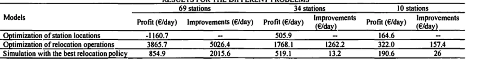
In Table 11, for each of the three network scenarios, results are compared for the solutions to the station location model without relocations [24], the solutions applying the relocation optimization model (1)-(8), and the best performing simulated relocation policiy.

Results for the simulated relocation policies are far from the optimal relocation solutions, showing that it is difficult to design effective real-time strategies based on fixed rules. A case in point is the 34 station scenario in which the optimized relocations contribute to an improvement in profit of about 1262 €/day, while the real-time relocation policies improve profit only to about 13 €/day.

Nevertheless, it is important to observe that the policies evaluated in this work were able to make profitable the 69 station scenario that serves all demand in the city. Relocation policies, then, can help carsharing companies to provide sustainable services to greater numbers of people in expanded geographic areas.

TABLE II

RESULTS FOR THE DIFFERENT PROBLEMS

69 stations 34 stations IO stations

Models _{Profit (€/day) Improvements (€/day) Profit (€/day) Improvements}

(€/day) Profit (€/day) Improvements (€/day) Optimization of station locations

Optimization of relocation operations Simulation with the best relocation policy

-I 160.7 3865.7 854.9 V. CONCLUSIONS 5026.4 2015.6

The most convenient carsharing systems for users are one way systems; however as detailed in the literature, these systems require vehicle repositioning to ensure that vehicles are located where they are needed ( 17], [21 ], [22]. Several approaches have been proposed to try to solve this problem, such as an operator-based approach [15], [16] and a station location approach [24]. With the operator-based approach, the stock of vehicles at stations is adjusted by relocating vehicles to locations where they are needed.

In this paper we present two independent tools that can be combined: a mathematical model for optimal vehicle relocation, and a discrete-event time-driven simulation model with several real-time relocation policies integrated. Kek et al. [15], [16] developed also an optimization model and a simulation model, but in their work only the optimization model allows determining the relocation operations. The simulation model is just used to evaluate the performance of the. sy�te�s when the relocation operations determined by the _{opt1m1zat1on model are performed. Nair and Miller-Hooks} [17] developed a stochastic mixed-integer programming model to optimize vehicle relocations, which has the advantage of considering demand uncertainty. However, they did not develop a simulation model and a way of determining relocation operations in real time. Barth et al. [18] presented a queuing based discrete event simulation model and three ways of deciding when relocations should be performed, one of which, called "Historical predictive relocation", is similar to what is proposed in the relocation policies presented here. Although, there is a higher number of policies and combination of parameters tested in this work than in [18]. Moreover, Barth et al. [18] did not develop an optimization

505.9 1768.1 1262.2 519.1 13.2 164.6 322.0 157.4 190.6 26

model and ways of combining both optimization and simulation. With respect to Barth et al. (19], an aggregated approach was developed. They only studied a measure to determine if the whole system needs relocations or not, while in this paper, each station is treated individually.

The developed optimization model was applied to the case study first introduced by Correia and Antunes [24]. Using the alternative networks of stations that were obtained for the city of Lisbon, the relocation approaches developed in this research were evaluated and compared.

The optimized relocation decisions for these networks indicated significant potential improvements in system profit. For instance, the solution covering all demand for the entire city ( containing 69 stations) has an estimated daily loss of 1160 €, but when operations are expanded to include optimal relocation decisions, this estimated daily loss is transformed into an estimated daily profit of about 3800 €. There are also significant economic improvements in the other networks (containing 34 and 10 stations).

Optimal solutions to the relocation model provide upper bounds on the economic gains achievable with relocations because inputs to the optimization model require a priori knowledge of the full pattern of daily trip demands. To evaluate the impacts of real-time relocation operations in this research, relocation policies were devised and executed in a simulation model. For the largest network of stations these simulated, real-time relocation strategies, are estimated to improve profitability significantly, reaching a profit of about

855

€/day with the best relocation policy. This is far from the optimum; however it is implemented real-time making it more likely to be achieved in the real operation when vehicles are not reserved one day in advance. For the smaller networks, the correspondingly smaller improvement is explained by the fact

(9)

that the station locations in these networks were specifically chosen to reduce the need for repositioning by using the model in [24]. By integrating results of the relocation optimization model with the relocation policies (for example, using in the simulation the optimization's initial vehicle availability at each station), improved results are achieved for the relocation policies.

The main conclusion that is drawn from this work is that relocation operations should be considered when setting up station-based one-way carsharing systems. An important effort must be made into studying more deeply what was defined in this paper as real-time relocation policies to be implemented in the day-to-day operation of these systems, thus allowing the sustainability of full network coverage of this service in a city. The fact that by introducing relocation policies it was possible to transform the worst profitable network (69 stations) into the most profitable encourages research into expanding the methods to estimate when and how many vehicles should be relocated between stations [29].

In what respects to the transferability of both models (mathematical model and simulation model) to another city, it is important to refer that mathematical models always have a computation time that is dependent on the problem dimension. Thus, as the city size increases, that is, the number of carsharing stations', the computation time should also increases due to the increasing number of decision variables. Regarding the simulation model, this problem is non-existent. Therefore, it can be applied to any city independently of its dimension.

Moreover, the results presented in this paper are very sensitive to changes in travel demand. So, the simulation model that was built in this work should be improved in future projects to increase the realism of the day-to-day operation of such transportation system, including stochastic trip variability and travel time.

ACKNOWLEDGMENT

The research in which this article is based was carried out within the framework of a PhD thesis of the MIT Portugal Program. The authors wish to thank the Portuguese Science Foundation for financing this PhD project through scholarship SFRH/BD/51328/2010. The authors would also like to thank the Portuguese Science Foundation for financing the InnoVshare project (PTDC/ECM-TRA/0528/2012).

REFERENCES

[I] D. Schrank, T. Lomax, and S. Turner, "TTl's 2010 Urban Mobility Report," Texas Transportation Institute, 2010.

[2] "National Household Travel Survey: Summary of Travel Trends," U.S. Department of Transportation, 2001.

[3] S. Shaheen, D. Sperling, and C. Wagner, "A Short History of Carsharing in the 90's," Journal of World Transport Policy and Practice, vol. 5, no. 3, pp. 16-37, Sep. 1999.

[4] T. Litman, "Evaluating Carsharing Benefits," Transportation Research Record: Journal of the Transportation Research Board, no. 1702, pp. 31-35, 2000.

[5] T. Schuster, J. Byrne, J. Corbett, and Y. Schreuder, "Assessing the potential extent of carsharing - A new method and its applications," Transportation Research Record: Journal of the Transportation Research Board, no. 1927, pp. 174-181, 2005.

[6] C. Celsor, and A. Millard-Ball, "Where Does Carsharing Work?: Using Geographic Information Systems to Assess Market Potential,"

Transportation Research Record: Journal of the Transportation Research Board, no. 1992, pp. 61-69, 2007.

[7] J. Schure, F. Napolitan, and R. Hutchinson, "Cumulative impacts of carsharing and unbundled parking on vehicle ownership & mode choice," presented at 91st Annual Meeting of the Transportation Research Board, Washington, DC, 2012.

[8] L. Sioui, C. Morency, and M. Trepanier, "How Carsharing Affects the Travel Behavior of Households: A Case Study of Montreal, Canada," International Journal of Sustainable Transportation, vol. 7, no. I, pp. 52-69, 2013.

[9] E. Martin, and S. Shaheen, "Greenhouse gas emission impacts of carsharing in North America," IEEE Transactions on Intelligent Transportation Systems, vol. 12, no. 4, pp. 1074-1086, Dec. 2011. [10] J. Firnkorn, and M. MOiier, "What will be the environmental effects of

new free-floating carsharing systems? The case of car2go in Ulm," Ecological Economics, vol. 70, no. 8, pp. I 519-1528, Jun. 2011. [11] S. Shaheen, A. Cohen, and J. Roberts, "Carsharing in North America:

Market Growth, Current Developments, and Future Potential," Transportation Research Record: Journal of the Transportation Research Board, no. 1986, pp. 116-124, 2006.

[12] M. Barth, and S. Shaheen, "Shared-Use Vehicle Systems: Framework for Classifying Carsharing, Station Cars, and Combined Approaches," Transportation Research Record: Journal of the Transportation Research Board,no. 1791,pp. 105-112,2002.

[13] C. Costain, C. Ardron, and K. Habib, "Synopsis of users' behaviour of a carsharing program: a case study in Toronto," presented at 91st Annual Meeting of the Transportation Research Board, Washington, DC, 2012. [14] D. Efthymiou, C. Antoniou, and P. Waddell, "Which factors affect the

willingness to join vehicle sharing systems? Evidence from young Greek drivers," presented at 91st Annual Meeting of the Transportation Research Board, Washington, DC, 2012.

[15] A. Kek, R. Cheu, and M. Chor, "Relocation Simulation Model for Multiple-Station Shared-Use Vehicle Systems," Transportation Research Record: Journal of the Transportation Research Board, no. 1986, pp. 81-88, 2006.

[16] A. Kek, R. Cheu, Q. Meng, and C. Fung, "A decision support system for vehicle relocation operations in carsharing systems," Transportation Research Part E: Logistics and Transportation Review, vol. 45, no. 1, pp. 149-158, Jan. 2009.

[17] R. Nair, and E. Miller-Hooks, "Fleet management for vehicle sharing operations," Transportation Science, vol. 45, no. 4, pp. 105-112, Nov. 2011.

[18] M. Barth, and M. Todd, "Simulation model performance analysis of a multiple station shared vehicle system," Transportation Research Part C, vol. 7, no. 4, pp. 237-259, Aug. 1999.

[19] M. Barth, J. Han, and M. Todd, "Performance evaluation of a multi station shared vehicle system," presented at IEEE Intelligent Transportation Systems Conference, Oakland, CA, 2001.

[20] D. Jorge, G. Correia, and C. Barnhart, "Testing the validity of the MIP approach for locating carsharing stations in one-way systems," presented at 15th Edition of the Euro Working Group on Transportation, Paris, 2012.

[21] W. Mitchell, C. Borroni-Bird, and L. Burns, "New Mobility Markets," in Reinventing the Automobile: personal urban mobility for the 21st century, Cambridge, MA, MIT Press, 2010, pp. 130-155.

[22] A. Febbraro, N. Sacco, and M. Saeednia, "One-way carsharing: solving the relocation problem," presented at 91st Annual Meeting of the Transportation Research Board, Washington, DC, 2012.

[23] W. Fan, R. Machemehl, and N. Lownes, "Carsharing: Dynamic Decision-Making Problem for Vehicle Allocation," Transportation Research Record: Journal of the Transportation Research Board, no. 2063, pp. 97-104, 2008.

[24] G. Correia, and A. Antunes, "Optimization approach to depot location and trip selection in one-way carsharing systems," Transportation Research Part E: Logistics and Transportation Review, vol. 48, no. I, pp. 233-247, Jan. 2012.

[25] H. Lau, "Network Flow," in A Java Library of Graph Algorithms and Optimiution, Boca Raton, FL, Chapman & Hall/CRC, Taylor & Francis Group,2007,pp. 254-272.

[26] iNTERFILE,

http://www.excel.interfile.de/Autokostenrechner/autokostenrechner.htm, Accessed June 10, 2012.

[27] car2go, http://www.car2go.com/, Accessed July 2, 2012.

[28] FICO, "Getting Started with Xpress ", Release 7. Fair Isaac Corporation, Leamington Spa, UK, 2008.

(10)

(29] D. Jorge, and G. Correia,. " Carsharing systems demand estimation and defined operations: a literature review," European Journal of Transport and Infrastructure Research, vol. 13, no. 3, pp. 201-220, s·ep. 2013.