Balancing a two-wheeled Segway robot

Balancing a Two-Wheeled Segway Robot

by

Maia R. Bageant

Submitted to the Department of Mechanical Engineering

in partial fulfillment of the requirements for the degree ofEiMASSACHUSETTS

OF TECHN!-tros y

Bachelor of Science in Mechanical Engineering

OCT

2 0 2011

at the

-T

U A

i

MASSACHUSETTS INSTITUTE OF TECHNOLOGY

ARCHNES

June 2011

©

Massachusetts Institute of Technology 2011. All rights reserved.

Author . ...

Department of Mechanical Engineering

May 6, 2011

7-v /

Certified by...

Harry Asada

Ford Professor of Engineering

Thesis Supervisor

Accepted

by..

Samuel C. Collins Profei

Balancing a Two-Wheeled Segway Robot

by

Maia R. Bageant

Submitted to the Department of Mechanical Engineering on May 6, 2011, in partial fulfillment of the

requirements for the degree of

Bachelor of Science in Mechanical Engineering

Abstract

In this thesis, I designed and constructed hardware for a two-wheeled balancing Seg-way robot. Because the robot could not be balanced based on a control system derived from the original analytical model, additional system dynamics in the form of frictional losses in the motors were incorporated. A SISO PID compensator and a SISO lead-lag compensator were designed to balance the robot based on the new model; both showed acceptable system responses but were subject to high-frequency oscillation. A SISO state feedback controller was also designed, and it was successful in creating stability in simulation and removing the high-frequency oscillation effects. The robot was rebuilt using new parts that better represented its ideal model, and software was created using National Instruments LabVIEW to control the robot. Thesis Supervisor: Harry Asada

Acknowledgments

The author would like to acknowledge her advisor, Professor Asada, for conceiving of the project and providing guidance during its execution; James Torres, for being readily available to procure hardware and answer questions of any sort; and her family, for supporting her through even the toughest of times.

Contents

1 Motivation ₁₃

2 Introduction and Background ₁₅

2.1 _{The Inverted Pendulum and Two-Wheeled Robots ... 15}

2.2 _{Physical Model of the Robot ... ... 16}

2.3 PID Control . . . . 18

3 Modified Model ₂₁ 3.1 _{Description of Modifications . . . . 21}

3.2 _{Modified Physical Model of the Robot . . . . 22}

3.3 _{Modified System Response . . . . 23}

4 Achieving Stability by Root Locus Shaping 27 4.1 W hy Root Locus? . . . . 27

4.2 _{Necessity of the Integrator . . . . 28}

4.3 _{Lead-Lag Compensator Design . . . . 30}

4.4 PID Compensator Design . . . . 32

5 Achieving Stability by Pole Placement 37 5.1 _{Derivation of the State Space Model . . . . 37}

5.2 Pole Placem ent . . . . 38

5.3 System Performance . . . . 40

6.1 B ody . . . . 43

6.2 D rive System . . . . 43

6.3 Sensors... ... ... . ... .. 44

6.3.1 Inertial Measurement Unit . . . . 44

6.3.2 Encoders . . . . 47 6.4 Processing Unit . . . . 47 7 Software Design 49 8 Conclusion 51 8.1 C onclusion . . . . 51 8.2 Further Study . . . . 52 A Numerical Constants 53

List of Figures

2-1 Diagram showing basic two-wheeled robot, with dimensions. . . . . . 2-2 Root locus for the plant. . . . .

2-3 _{Root locus for the plant with PD control. . . . .}

3-1 _{Modified diagram showing parasitic torques. . . . .} 3-2 Root locus for the modified plant. . . . . 3-3 Effects of single poles or zeroes on the root locus. PD control is shown

to be inadequate. . . . . 4-1 _{Frequency response for the modified plant. . . . .} 4-2 Frequency response for the modified plant with a PD controller. . . .

4-3 Effect of adding an integrator to the plant. 4-4 4-5 4-6 4-7 4-8 4-9 5-1 5-2 5-3

Root locus for lead-lag compensated system. . . . . Response of lead-lag compensated system to pulse signal. Controller effort for lead-lag compensated system... Root locus for closed loop PID compensated system. Response of PID compensated system to pulse signal. . .

Controller effort for PID compensated system. . . . . Pole-zero map of the system with state feedback... Response of state feedback system to pulse signal... Control effort for state feedback system. . . . .

. . . . 3 0 . . . . 32 . . . . 33 . . . . 34 . . . . 35 . . . . 36 . . . . 36 . . . . 39 . . . . 40 . . . . 41

6-2 Neutral voltages for the various orientations of the accelerometer. The

leftmost orientation is the one selected for this application. . . . . 46

List of Tables

A.1 Robot body.. ... 53 A.2 Motor. ... 53 A .3 Sensors. . . . . 53

Chapter 1

Motivation

The motivation for this project stems from a laboratory assignment given in the course 2.12 Introduction to Robotics. In the final lab module of the course, students were given the opportunity to design a control system to balance a two-wheeled Segway-style robot. However, despite the efforts of the course staff during preparation for this assignment, the physical robot on which the students were to test their control systems could not be balanced. During class a simulation was used instead.

For the course in the fall of 2011, it was desired to improve the hardware to allow it to be balanced by the students. The work described in this document was completed with the aim of revising the physical model and improving the hardware and software in order to allow balancing stability of the robot to be achieved by future students.

Chapter 2

Introduction and Background

2.1

The Inverted Pendulum and Two-Wheeled Robots

The inverted pendulum is a system frequently analyzed both inside the classroom and out. It is commonly described as a pendulum, or a rigid rod with a bob on the end, mounted by a hinge to a cart, which can be translated along a track by an input force. The pendulum itself, however, is not actuated; it is free to swing around its point of marginal stability in the vertical position. Only by properly actuating the cart and using the reaction force of the pendulum against the cart can the pendulum be positioned.

In this feature lies the significance of the inverted pendulum. It is an indirectly actuated system-that is, the object of interest, the pendulum, can be controlled only

by exerting a force on the secondary object, the cart. The novelty and challenge of

implementing such a controller in the real world has attracted attention from many parties, not the least Dean Kamen, whose Segway personal transportation device, revealed in 2001, is at its heart a two-wheeled pendulum, designed both to balance upright and to translate the rider and device to a new position [3].

Perhaps because of the fame of the Segway, two-wheeled balancing robots have become a prominent project for students and hobbyists. It is certainly a topic of interest to anyone involved in the study of control systems and their application to robotics.

2.2

Physical Model of the Robot

The two-wheeled robot consists of a long body with two wheels mounted at one end. For the simplicity of this derivation, the two wheels will be treated as a unit, and it will be assumed that the robot travels only in a straight line.

By properly designing the hardware, modeling can be simplified. Thus, the body

can be treated as a point mass, rotating about the axis of the wheels. The set of assumptions made to simplify modeling is as follows:

" The wheels are always in contact with the floor and experience rolling with no

slip;

" The electrical and mechanical losses can be approximated to zero;

* The electrical system response is significantly faster than that of the mechanical system, so the dynamics of the electrical system may be neglected;

* The motion of the robot is constrained to a straight line, so that the system may be analyzed as a 2-dimensional system with only planar motion;

" All bodies are rigid;

" The angle of tilt from the vertical of the upper body is sufficiently small to allow

linearization of the system (sin(62) ? 02);

" And the angular velocity of the tilt of the upper body is sufficiently small

(62 ~ 0) such that the centrifugal force may be neglected.

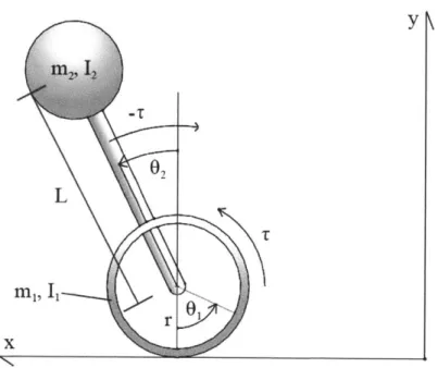
Under these conditions, the robot can be modeled as shown in Figure 2-1. The equations of motion resulting from this case are derived as the following:

T = H101 + H362 - m2rL sin(62)#

- T = H301 + H262 - mgL sin62,

L

i,

Ii-x

Figure 2-1: Diagram showing basic two-wheeled robot, with dimensions.

H

F

I

[

H

H

J

[

m

rLcos

m

L

+ 12

I1 and 12 are the rotational moments of inertia of the wheel and the robot body,

respectively; r is the radius of the wheels; L is the length between the center of mass of the body and the wheel axis; and in and m_{2 are the masses of the wheels and the}

robot body, respectively.

Linearization of these equations, based on the conditions listed above, yields the following equations of motion:

T H01 + HA62

2.3

PID Control

Based on these equations of motion, the input command takes the form of the torque,

T, and the output may be either the position of the wheels, 01, or the tilt angle of the body, 02. In order to achieve balancing stability, the desired output is 02.

The transfer function from r to 02 is thus given by:

_ 02 _ -(H + H3)

T Ds2-aH ₁

where a = m2gL.

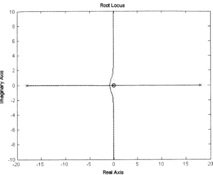
The root locus stemming from this transfer function is shown in Figure 2-2.

Root Locus

-8 -60 -40 -20 0 20 40 60

Real Axis

Figure 2-2: Root locus for the plant.

The controller design for this system is fairly straightforward. The root locus contains two zeroes symmetric about the imaginary axis. A proportional-derivative (PD) controller may be applied, reshaping the root locus and drawing it into the left

half-plane, as shown in Figure 2-3. At this point there is a great degree of freedom to tune the system response in order to achieve the desired balancing performance.

Root L oc u EdIfr opn op. 1 L

-4ii -20

Figure 2-3: Root locus for the plant with PD control.

19 -1610 -140 -120 -10

Chapter 3

Modified Model

3.1

Description of Modifications

Though the model described in Section 2 was applied to the two-wheeled robot in question, stability could not be achieved. A likely source of this instability was losses in the motors. These losses can be attributed to both mechanical and electronic effects.

The mechanical losses were estimated using an expression provided by the bearing manufacturer SKF [4]. According to this equation, the equivalent coefficient of sliding friction for a bearing can be calculated using a weighted sum of coefficients of friction for various types of contact and lubrication. This value was calculated for rotational speeds between 0 and 100 rpm and used to determine the frictional moment at these speeds. A linear fit for rotational speed versus frictional moment was found. The slope of this linear fit gave b, the coefficient of mechanical loss. See Appendix B for more information on how this value was determined.

Electrical losses were neglected, as they cannot be modeled as directly propor-tional to w. Power dissipated is given by the expression

R

Pdw s m can b

curve of the motor:

Pds = R(rst - K2u)2.

Kt

Thus, electrical losses are not a linear function of w, and will be neglected in this model.

The mechanical damping coefficient, then, can be represented as viscous damping, which is proportional to the relative velocity between the wheels and the body. The parasitic torque lost due to frictional damping can thus be modeled by the expression:

,ioss = b(0 2 - 01).

With this knowledge, the equations of motion can be revisited, and these losses worked into the system dynamics.

3.2

Modified Physical Model of the Robot

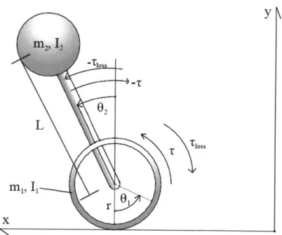
Now, the equations of motion can be revised to incorporate the frictional losses within the motors. The losses appear as a parasitic torque acting in the generalized forces; as such, the revision to the equations is fairly straightforward, as T is replaced byT + 7Ts:

Trevised T r + Toss = r + b(0 2 -

01)-The revised equations of motion are thus:

T +

Z7-N

Tloss

Figure 3-1: Modified diagram showing parasitic torques.

3.3

Modified System Response

As in Section 2.3, the input is the torque T, and the desired output for balancing

control is 02. By taking the Laplace transform, substituting, and rearranging, the

equations can be manipulated to show that the transfer function of interest is:

G2(8) = 02 _ (Hi + H3)s

T (H₁H2 - H2)s 3+b(Hi + H2 + 2H3 )s2 - aH1s - ab

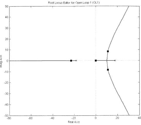
Note in this transfer function that there are now three poles instead of two, and one zero. Thus the system order remains the same, but the parasitic effects of the losses have manifested as a zero at the origin. The open loop system is unstable, as expected.

However, achieving stability in this root locus is more difficult than in the previous case. Due to the presence of the zero at the origin, the section of the root locus in the right half-plane cannot be drawn into the left half-plane in order to achieve stability.

Root Locus

.15 -10 -5 0 5 10 15 2

Real Axis

Figure 3-2: Root locus for the modified plant.

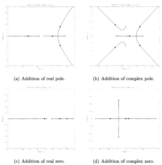
No application of a PD controller can achieve stability; placing the zero in the right half-plane only reinforces the instability, and placing it in the left half-plane has no effect on the unstable region.

(a) Addition of real pole. (b) Addition of complex pole.

(c) Addition of real zero. (d) Addition of complex zero.

Figure 3-3: Effects of single poles or zeroes on the root locus. PD control is shown to be inadequate.

Chapter 4

Achieving Stability by Root Locus

Shaping

4.1

Why Root Locus?

There exist many tools to an engineer designing a control system. Why choose to design for stability using the root locus? There are several reasons that make the root locus apt to selecting the type of controller to be utilized: it is a simple and visual design tool that is quickly and easily generated; the stability of the system is reliably represented; and an idea of how changes to the controller affect the overall stability of the system can be quickly perceived. The root locus has limitations; the numerical computations required to tune system performance to the desired level can require iteration, and it is difficult to numerically optimize the system response via root locus design.

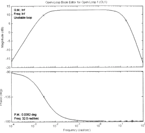
Another reason that design by root locus was chosen for this case is that for this particular system, design by loop shaping using the magnitude and phase frequency response is ambiguous. As shown in Figure 4-1, there are two crossover points; while the first is stable, the second seems to be unstable. Addition of a PD controller shows some difference in the frequency response-however, the phase margin at both crossover points is positive, belying the fact that the system is, in fact, unstable. This fact is shown in the plots in Figure 4-2.

Cren-Loop Bode Editor for Oipen Loop 1 (L 1 15 ---G.M.: Inf 10 C- Freq: inf Unstable loop M, ₀ -P.M.: 0.0382 deg Freq: 32.5 red/sec -2 , -1 10 10 1r 1I- 10 1: 10 Freqcyr~r (rad/sc)

Figure 4-1: Frequency response for the modified plant.

Thus, in order to select a controller that may later be tuned, the root locus is a perfectly suitable tool. It gives an instantaneous evaluation of whether stability can be achieved, and allows the system to be quickly and easily manipulated before detailed tuning is undertaken.

4.2

Necessity of the Integrator

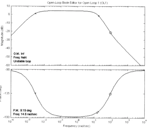
From the root locus shaping described in Section 3.3, it is apparent that the system cannot be made stable using PD control, as the lossless system can be. In fact, application of any one real or complex zero or pole is unable to draw the root locus into the stable region. This is because of the zero; as it serves as a sink, it is impossible to draw the root locus away from it without forcing the segment associated with the right half-plane pole to remain unstable.

ipen-Loop Bode Editor fot ren Loop 1 (OLI 0--10 ' ~ 0 _40 G.M.: Inf 5I Freq: NaN Unstable loop -60j P.M.: 9.19 deg Freq: 14.8 rad/sec 10 12 -1 .100 1 2 324 Frequency' (arid/sec)

Figure 4-2: Frequency response for the modified plant with a PD controller.

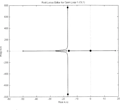
The next tactic available to the designer is to cancel the zero at the origin using an integrator. In design practice, canceling zeroes and poles is typically a poor decision. This is because in application to real systems, poles and zeroes can drift due to changes in the system and its environment. If the canceling singularity drifts away from the canceled, the undesirable system dynamics can return.

However, in this case, the zero is at the origin, and is unlikely to drift due to the fact that the losses are modeled as viscous damping and purely dissipative. This means that application of a pole to the origin in order to cancel the offending zero is an acceptable design decision, and in fact the simplest way to draw the root locus into the left hand-plane.

Root Locus Editor for Open Loop 1 (.L1

40-2A

150

--80 0 -40 0 2 40

Figure 4-3: Effect of adding an integrator to the plant.

4.3

Lead-Lag Compensator Design

The lead-lag compensator is often applied to alter an undesired frequency response of a system. In this case, it is applied as a variation on proportional-integral-derivative (PID) control. The advantage in this situation of using the lead-lag controller is that all poles and zeros can be placed on the real axis, and oscillation can thus be eliminated from the system. In addition, the extra pole gives the system another dimension that can be tuned, and a greater control of the system response can be obtained.

Due to the presence of the zero at the origin, one pole was selected to be at the origin, canceling it and serving as the integrator. This serves as the root of the lag compensator. To place the zero of the lag compensator, it was desirable to place it as close as possible to the left half-plane pole of the smallest magnitude without surpassing this pole in magnitude.

Surpassing the pole in magnitude caused the root locus to branch, introducing low-frequency oscillation in the system. Since one reason behind choosing the lead-lag controller was to remove oscillation from the system, this option was avoided. The zero was thus placed close to the pole while still allowing some room for it to drift (10% drift was deemed acceptable based on inaccuracies in measuring physical values).

Selecting these locations for the pole and zero of the lag compensator effectively break the root locus up into two real-axis segments, each stemming from a pole and ending in a zero with no branching. It is further desirable to place the lead compensator's pole and zero to continue this pattern. To this end, the zero of the lead compensator was placed on the real axis and to the right of the left half-plane pole of greater magnitude, again within 10% of that pole.

The zero of the lead compensator was then placed to the left of this system pole. The benefit of this placement is that this zero can control the bandwidth of the system independently. This does cause the system to branch at this high frequency, but high frequency oscillation was deemed less problematic than low-frequency oscillation, since it could be removed fairly simply by applying a low-pass filter, or by letting the electromechanical system itself act as a low-pass filter.

After placement of these poles, it was determined for the physical system at hand that the following transfer function created an acceptable system response:

G2(8) = 3300(1 + 0.062s)(1 + 370s)

s(1+0.02s)

A pulse signal of magnitude of 1 radians and of duration 0.4s was applied to the

system; this was intended to mimic an impulse disturbance, as the robot was pushed, rolled over a bump in the floor, etc. The system response is shown in Figure 4-5.

However, as evident in the transfer function above, the gain required to achieve this performance is very high. Though the system follows the signal quickly, it displays significant high-frequency oscillations. Examination of the control effort shows that if the output were limited to ±6 V (or the corresponding ±2.5 Nm of torque), stability

Root Locus Editor for Open Loop 1 (L1) 600 400- 200-.1 0 E -400 -61 -50 -40 -30 -2 -10 0 10 20

Figure 4-4: Root locus for lead-lag compensated system.

could still be achieved, but that the system response was not ideal.

This model was thus deemed acceptable for application to the system, but other potential controllers were also investigated.

4.4

PID Compensator Design

The lead-lag controller designed to eliminate oscillation while promoting stability did indeed eliminate low-frequency oscillation, but not high-frequency. To investigate whether shifting the oscillations to low frequency produced a more satisfactory system response, a proportional-integral-derivative (PID) controller was also designed.

Root locus shaping was again used to establish the basic compensator form. The integrator was again used to cancel the zero at the origin. A complex zero was then placed in the left half-plane; this successfully drew the asymptotal branches of the resulting root locus into the left half-plane. With a sufficiently high gain, the

closed-x10 9 8 -. 7-6 <3 2 1 -- 0--1 ' I I I I 0 0.1 0.2 0.3 0.4 0.5 0.6 0.7 0.8 0.9 1 Time, s

Figure 4-5: Response of lead-lag compensated system to pulse signal. loop system was predicted to undergo stable oscillations.

However, a lightly damped system was undesirable, as lightly damped oscillation about the balance point did not represent ideal "stability." A damping coefficient of

0.707 was thus selected. In addition, the settling time was selected to be less than 0.5 s. This was to ensure that the system would quickly reject disturbances and return

to its point of marginal stability rather than continuing to oscillate.

Thus, the location for the complex zero created by the PID controller was at

s = _{-8 ± 8j, and the transfer function describing the resulting controller was:}

G2(s) = 17, 000 (S2 + 16s + 128)

S

This system showed a response similar to that of the lead-lag compensator, but the oscillations were, as expected, of much lower frequency. The response to the pulse signal utilized in the previous section is shown in Figure 4-8.

Though these conditions created stability, the low-frequency oscillation looked like it would create an undesirable response, as the robot would "twitch" back and forth

0.5 E 0 -1 -1 5.5 . . . . 1 0 0.1 0.2 0.3 0.4 0.5 0.6 0.7 0.8 0.9 1 Time, s

Figure 4-6: Controller effort for lead-lag compensated system.

around its point of stability. The control effort was acceptable, as shown in Figure 4-9. In addition, there was still a high-frequency "ringing" present, which seems especially undesirable in the control effort.

Both of these controllers were deemed to have acceptable performance, given that a low-pass filter can remove the undesirable high frequencies, but another design tool remains available that gives the designer the option to further adjust performance: state space design.

Root Locus Eciftor for O-pen Loop I (OL1

-60 -50 -4u -30 r-20

Real AdS

-10 0 10 2110

Figure 4-7: Root locus for closed loop PID compensated system.

-101

-70

x 10

4

r-Time, s

Figure 4-8: Response of PID compensated system to pulse signal.

-0.5

-1

-1.51-0 0.1 0.2 0.3 0.4 0.5 0.6

Time, s

Chapter 5

Achieving Stability by Pole

Placement

5.1

Derivation of the State Space Model

Both SISO controller designs described in Section 4 were able to create stability within the limitations of the effort that the hardware could supply. However, to investigate if an even more satisfactory response could be produced, the next iteration of the design was constructed with a state feedback controller.

Though a state feedback controller is capable of handling multiple input, multiple output systems, for balancing control, only one input, torque r, and one output, angle 02, _{are to be controlled. Thus it is convenient to design a SISO state feedback}

controller to achieve balancing stability.

Recalling the transfer function for balancing control from Section 3:

G2(8) = = (Hi + H3)s

G ( H1H2 - H)s3 + b(H1 + H2 + 2H3)s2 - aH₁s - ab

By cross-multiplying and taking the inverse Laplace transform, the time-domain

equa-tion describing the relaequa-tionship between T and 02 can be determined:

(H1H2 - H2)-02 + b(H1 + H2 + 2H3)52 - aH192 - a02 - (H1 + H3)+

From this equation, the matrices required for the state space representation can be derived. This representation is thus given by:

02

[

+2H

)

aH

a

1H2-Hj

The state variables for this case consist of 92, 92, and 92.

5.2

Pole Placement

In the terms of root locus shaping, SISO controller design consists of adding poles and zeroes to the existing singularities of the plant root locus. Full state feedback, however, allows the technique of pole placement to be utilized. This means the existing poles of the plant can be moved around the complex plane to any desired location.

State feedback does require certain conditions to be successful. First, the states must either be measured or estimated successfully. The downside of this condition is that multiple sensors may be needed in order to create a sufficient number of feedback states, potentially increasing the cost and complexity of the hardware. Second, the measurement of the states must be sufficiently accurate and noise-free, or the system response deteriorates.

However, at least one sensor is already necessary for PID control; in this case, the feedback variable, 92, must be measured in order to be fed back. And, if the signal

to estimate unmeasured states 02 and 02 should pose no problem. (As designed, the robot incorporates sensors that can measure both 02 and 02 directly.)

With that fact, design of the state feedback controller can commence. The offend-ing pole is the one located in the right half-plane. By the techniques of root locus shaping, it is desirable to move it into the left half plane, onto the real axis. (In gen-eral, leaving singularities alone reduces the dependence of the system on numerical accuracy, since the stationary poles are inherent to the system rather than numeri-cally calculated based on the feedback gains. If the system response is unacceptable, however, they may be moved via pole placement.)

Placement of poles can also adjust the properties of the closed-loop system; most importantly, the speed of the system's response. It was determined based on the existing hardware that the pole closest to the origin was extremely slow, with a response time on the order of 300 s. Thus, this pole was moved to s = -10, in

order to improve the system response time, and the unstable right half-plane pole

was moved to s = -100. Pole-Zero Map 0 -0.6 021 -0.4 00 -80 -60 -40 -20 0 Real Axis

Figure 5-1: Pole-zero map of the system with state feedback. The state feedback gains resulting from these design decisions were:

K = 2 8338 10, 1081

5.3

System Performance

The system performance resulting from pole placement and state-space design also showed a quick rejection of disturbance and return to stability. The test signal was identical to the pulse described in Section 4. The response time was relatively slow compared to the PID and lead-lag controllers, at approximately 0.25 s. However, all oscillation-both the high-frequency ringing and the low-frequency oscillation about the point of stability-are removed. This eliminates the need for a low-pass in this case, and greatly simplifies controller design by giving the designer the freedom to independently adjust parameters.

0 0.5 1 1.5 2 2.5

Time, s

3 3.5 4 4.5 5

Figure 5-2: Response of state feedback system to pulse signal.

The final test was to determine if real-world limitations such as saturation would

0.4 0.2 0 --0.2 -E -0.4 -Ti -0.6 -E -0.8 --1 -1.2 I I I I | | | | 0 0.5 1 1.5 2 2.5 3 3.5 4 4.5 5 Time, s

Figure 5-3: Control effort for state feedback system.

prevent the system from achieving stability. However, upon examining the control effort required, it became apparent the saturation was unlikely to become a problem, as shown in Figure 5-3. The torque required never exceeded 1.5 Nm in magnitude.

Overall, the state feedback controller showed excellent results, and is the recom-mended method of implementation.

Chapter 6

Hardware Design

6.1

Body

To attempt to make the task of balancing the robot even easier, the hardware was designed to mimic the idealized model described in Section 3. Thus, the body con-sisted of a half-inch thick sheet of acrylic. The processing unit, which was contained in a heavy cast metal case, was mounted at the top, serving as the point mass for the pendulum bob. The midsection of the robot was cut out to reduce its relative weight. The wheels were mounted at the bottom, directly underneath the processing unit. The point of stability of the robot could then be adjusted by bolting additional material onto the head opposite the processing unit; without any additional material, the point of neutral stability was within 1 cm of vertical.

6.2

Drive System

The drive system consisted of two independent DC servo actuators manufactured

by Harmonic Drive Systems, Inc., of specification RH-11D, mounted directly to the

wheels. The motors are each capable at 12 V of exerting 2.4 Nm of torque at stall and have a maximum rotational speed of 100 rpm, giving an idealized torque-speed curve shown in Figure 6-1 [2].

resis-(a) Image of the front of the robot; note the hol- (b) Image with the main components of the

lowed out midsection. robot labeled.

tance of the armature R is measured to be 4.7Q, and thus the torque constant Kt can be calculated to be Kt = vT/iKm = 1.483Wb.

6.3

Sensors

6.3.1

Inertial Measurement Unit

The inertial measurement unit (IMU) purchased from SparkFun Electronics consisted of a two-axis accelerometer, Analog Devices ADXRS401, and a yaw rate-measuring gyroscope, the Analog Devices ADXL320. Mounting the sensor vertically as shown allowed 62 and 62 to be measured directly.

The yaw rate measured at the motor axis gives a direct measurement of 62. At rest, the gyro gives a voltage of 2.5V; depending on which direction it is rotated, when moving, it deviates from 2.5 V by a rate of 15 mV per degree per second, or 859.437mV per radian per second [5]. (See Figure 6-2.) In addition, the positive direction of the gyroscope corresponds to the negative direction of 62. Therefore, 62 can be calculated by the expression

Torque-Speed Curve for Harmonic Drive Inc RHD-1 I 6 I I I I 5 5 N 3 N N N I N N. N I I I I I I I I I 4. ZI. 1. tJ. 8 9 10 11 12

Figure 6-1: Idealized torque-speed curve for the RH-11D motors.

-(Vmeasured - 2.5V)

02 - 859.437mV/rad/s

Then, 02 can be measured by either integrating 02, or by taking the arctangent of the y-acceleration over the x-acceleration. Because the acceleration due to gravity causes an offset in the vertical mounting orientation, the y-voltage is 3.5V at rest, and the x-voltage at 2.5V [1].

Though the sensitivity of the accelerometer is 312 mV per gravity of acceleration, this conversion factor cancels when the inverse tangent of the values is taken:

02 =

arctan

("

-TV - 2.5Vm

Though 62 may also be integrated to find062 (instead of measuring 02 directly),

1 2 3 4 5 6 7

Speed- rad s

PIN 8

XOUT = 1,5V

YOUT = 2.5V

JT C

UUU

_UUU,

PIN$ 8

TOP VIEW

PIN 8

XOUT= 2.5V (Not to Scale) XOUT 2.5V

YOUT

=3.5V

I nn

Yogy

YU31.5V

TOU 3,95VT 25

XXoUT = 3.5V

YOUT =

2.5V

EARTH'S SURFACE 3

Figure 6-2: Neutral voltages for the various orientations of the accelerometer. The leftmost orientation is the one selected for this application.

over time error tends to accumulate, so utilizing a Kalman filter and the measured 62

and 62 states instead of plain integration is another option.

Mounting the sensor at the base of the robot, near the wheel axis, is beneficial for several reasons. One reason is that by placing the yaw rate sensor nearly at the motor axis, 62 can be more accurately measured. The second is that the linear accelerations measured by the accelerometer are proportional to their distance from the wheel axis; if mounted near the axis, the voltages output by the device are low, and saturation is unlikely to be a problem. Finally, it is desired to measure the angle by measuring the change in the direction of gravity; small variations in acceleration due to the movement of the robot are less prominent when measured near the wheel axis, so noise is reduced.

The sensor was mounted on a breadboard and wired directly to the processing unit Analog In module. The x-accelerometer output was fed into the AIO port, the y-accelerometer output into the All, and the gyro output into the AI2 port.

6.3.2

Encoders

Encoders are built into each motor. They are classified as Optical Encoder ME-02-0, and are rated at 1000 pulses per rotation. These encoders can measure the change in angle between the wheels and the body.

However, this means that the encoder measurement alone cannot be used to dis-tinguish 01, the position of the wheels, and 02, as motion in either 01 or 92 will affect

the encoder reading.

Thus, if driving control were to be implemented, the 92 measured by the IMU

could be subtracted from the encoder reading to compute 61. For balancing control, the data from the encoders is not essential.

6.4

Processing Unit

The processing unit utilized was a National Instruments Compact RIO 9074, with three modules (two Brushed DC Motor Driver NI 9505 modules, and one Analog Input

NI 9205 module). The processor was run in field programmable gate array (FPGA)

mode, and power was provided using a 20 V DC power supply. Communication between a computer and the cRIO was accomplished by using a CAT-5 crossover cable. All motors and sensors were wired directly into the cRIO modules.

Chapter 7

Software Design

The software utilized was National Instruments LabVIEW 2009. Because the pro-cessor was also National Instruments hardware, the integration was straightforward. The design of the software was focused on providing a user interface that could be tweaked to allow students to observe the performance of the state space controller and to design their own controller.

A backend FPGA virtual instrument (VI) was created to handle the direct input

and output control of the cRIO microcontroller. This VI communicated with the frontend VI, which contained the blocks necessary to create balancing control.

The VI was structured in such a way to allow two different control modes to be implemented. The state space model was entered manually in a MathScript node. This model was then passed into a linear quadratic regulator, which calculated the optimal state feedback gains. Another input block allowed the student to input their own selection of feedback gains. Selecting the control mode (user-input or automatically calculated) was performed by switching a toggle on the front panel.

Once a control mode was selected, the chosen feedback gains were used to amplify the measured state. From the gyroscope, 62 _{was measured; from the accelerometer,}

62 was measured; and by differentiating the gyroscope signal, 62 was measured. The gyro in particular showed a great deal of noise, so a low-pass Butterworth filter was used to filter the signal.

noisy measured states with estimated states. Toggle switches on the front panel allowed the Kalman states to be turned on and off.

The selected states were then combined into a final state vector, which was passed to the controller.

After applying the state feedback gains to the state vector, the input torque T

necessary was calculated. However, the command to the motors needed to be a voltage, not a torque. Using the motor torque constant and resistance, the torque command was scaled into a voltage command, which was sent to the FPGA via an

FPGA write block.

Below is shown a schematic of how the software operates. The link between the motors and the sensors (that is, the physical robot) is not shown.

Chapter 8

Conclusion

8.1

Conclusion

In conclusion, it was determined that though PD control was sufficient to achieve stability for the system in which frictional losses were considered negligible, it was insufficient for the case where frictional losses were significant. Using the technique of root locus shaping, two new controllers were designed for this modified case.

The first was a lead-lag controller. The design of this controller was such that the dominant poles were on the real axis to prevent low-frequency oscillation. The response and required control effort of the lead-lag compensated system to a dis-turbance torque were calculated and deemed acceptable, except for the presence of significant high-frequency oscillation.

The second controller was a PID controller with a complex zero. The design of this controller was based on the idea that moving the oscillation from the high-frequency range to the low-high-frequency range might produce a better system response. The response and required control effort of this system were again satisfactory, though low-frequency oscillation of a small magnitude was present. However, though the high-frequency oscillation was reduced in magnitude, it was still present in the system response.

To create a more satisfactory system response, state feedback control was imple-mented. Using pole placement, the unstable pole was moved to the left half-plane,

and the pole near the origin that limited the speed of system response was moved to a higher natural frequency. The system response for the state feedback system was the most satisfactory of the three, as the system quickly rejected disturbance torques with no oscillation whatsoever.

Once the controller had been determined, it was implemented in hardware form.

A new robot was constructed so that its properties mimicked the idealized model as

closely as possible. The robot was equipped with an encoder on each servo motor, and an inertial measurement unit consisting of a two-axis accelerometer and a gyroscope. Software to run the robot was constructed using National Instruments LabVIEW; this software was based on the state feedback controller, and allowed users to select whether they wanted linear quadratic regulator-calculated optimal state feedback gains, or user-input state feedback gains. It also incorporated a Kalman filter to allow state estimation to replace input from particularly noisy sensors.

8.2

Further Study

Though the control system was designed and tested in simulation and the hardware was constructed, the controller was never successfully tested on the hardware. Due to time constraints, the software was still in the debugging phase at the time of this writing, with the main problems occurring in the communication between the software and the FPGA unit during runtime. It is believed that given more time the author could have completed the debugging phase and successfully balanced the robot.

In addition, this controller applied only to balancing control. Driving control requires further investigation. In SISO form, the driving control can be modeled as an external loop around the balancing internal loop. In state space form, the state vector changes to include 01 and 61. Thus, designing a straight-line driving control would require the design process to begin anew, effectively for a totally new plant. Furthermore, if the robot is to turn, then each wheel must be controlled independently, further complicating the compensation necessary. If this project were to be developed further, any of these features would be worthy pursuits.

Appendix A

Numerical Constants

Table A.1: Robot body.

Km 0.684mkg1/2 /,1/2 Kt 1.483 Wb R 4.7 Q Tma2 4.9 Nm Wmax 100 rpm Table A.2: Motor.

Gyroscope rate 15 mv/o1.

Gyroscope neutral voltage 2.5 V

Accelerometer rate 312 mv/g

Accelerometer neutral x voltage 2.5 V Accelerometer neutral y voltage 3.5 V

Encoder rate 1000 Pulses/rev

Appendix B

Calculation of Frictional Losses

The coefficient of friction for the bearing was calculated using a formula given by the bearing manufacturer SKF [4]. According to this formula, the coefficient of friction for a bearing is a function of the weighted average of several coefficients of friction that describe friction inside the bearing under various contact and lubrication conditions. SKF conveniently provides a utility to calculate the frictional moment for a partic-ular bearing. Given the rotational speed, the load on the bearing, and the coefficient of friction, the total frictional moment could be determined by adding the frictional moment for each source of loss. Cylindrical roller bearings of diameter 0.75 inches were chosen as representative of those found inside the motors; the load applied to the bearings was estimated at 50N; and the rotational speed was iterated by 10 from

0 to 100rpm. These points were plotted on a scale of rotational speed versus total

frictional moment, as shown in Figure B-1.

The line is nearly linear at these relatively low rotational speeds, so a linear fit was deemed appropriate. The slope of the line was calculated to be

0.071Nmm/rpm = 6.71 X 10-4Nm/rad/s,

exactly the correct units for the coefficient of damping, b.

For simplicity, b was estimated at 1 x 10-3Nm/rad/s, due to the fact that there are

Total Frictional Moment for Characteristic SKF Bearing

5-0

- 0

0

Rotational Speed (u), rpm

Bibliography

[1] Analog Devices, "Precision t1.7g Single/Dual Axis Accelerome-ter," ADXL103/ADXL203 datasheet, 2004. [Online]. Available: http: //www.sparkfun.com/datasheets/Accelerometers/ADXL203.pdf. [Accessed: April 2011].

[2] Harmonic Drive, LLC, "Actuators: RH Mini Series," Harmonic Drive, LLC, 2011. [Online]. Available: http://harmonicdrive.net/products/actuators/ rh/. [Accessed: April, 2011].

[3] Segway Inc., "About Segway: Segway Company Milestones," Segway Inc., 2011. [Online]. Avaliable: http://www.segway.com/about-segway/ segway-milestones. php. [Accessed: April, 2011].

[4] SKF Group, "Friction: The new SKF model for calculation of the frictional moment-Mixed lubrication for low speeds and viscosities," SKF Interactive

Engineering Catalogue. [Online]. Available: http: //www. skf .com/portal/skf /

home/products?lang=en&maincatalogue=1&newlink=1_0_38b. [Accessed:

April 2011].

[5] Spark Fun Electronics, "IMU Combo v2," ADXRS/ADXL combo datasheet,

2005. [Online]. Available: http://www.sparkfun.com/datasheets/