Are learned molecular representations ready for prime time?

Are Learned Molecular Representations Ready for

Prime Time?

by

Kevin Yang

Submitted to the

Department of Electrical Engineering and Computer Science

in Partial Fulfillment of the Requirements for the Degree of

Master of Engineering in Electrical Engineering and Computer Science

at the

Massachusetts Institute of Technology

June 2019

c

○ Massachusetts Institute of Technology 2019. All rights reserved.

Author:

Department of Electrical Engineering and Computer Science

May 24, 2019

Certified by:

Regina Barzilay, Delta Electronics Professor, Thesis Supervisor

May 24, 2019

Accepted by:

Are Learned Molecular Representations Ready for Prime

Time?

by

Kevin Yang

Submitted to the Department of Electrical Engineering and Computer Science on May 24, 2019, in Partial Fulfillment of the Requirements for the Degree of

Master of Engineering in Electrical Engineering and Computer Science

Abstract

Advancements in neural machinery have led to a wide range of algorithmic solutions for molecular property prediction. Two classes of models in particular have yielded promising results: neural networks applied to computed molecular fingerprints or expert-crafted descriptors, and graph convolutional neural networks that construct a learned molecular representation by operating on the molecular graph. In this paper, I benchmark models extensively on 15 proprietary industrial datasets spanning a wide variety of chemical endpoints. In addition, I introduce a graph convolutional model that consistently outperforms models using fixed molecular descriptors as well as previous graph neural architectures on both public and proprietary datasets. Our empirical findings indicate that while approaches based on these representations have yet to reach the level of experimental reproducibility, the proposed model nevertheless offers significant improvements over models currently used in industrial workflows. In addition, I demonstrate that similar models show promise in the molecular generation setting.

Thesis Supervisor: Regina Barzilay Title: Delta Electronics Professor

Acknowledgments

I thank the coauthors of my forthcoming paper of the same title[51], upon which this thesis is based: Kyle Swanson, Wengong Jin, Connor Coley, Regina Barzilay, Tommi Jaakkola, and Klavs Jensen at MIT; Philipp Eiden, Miriam Mathea, Andrew Palmer, and Volker Settels at BASF; Hua Gao, Timothy Hopper, and Angel Guzman-Perez at Amgen; and Brian Kelley at Novartis. Many sections from that paper are reproduced in this thesis with minor modifications. In particular, much of my work this year has been done together with Kyle Swanson.

I thank the Machine Learning for Pharmaceutical Discovery and Synthesis con-sortium for funding this research.

In addition, I would like to thank the other members of the computer science and chemical engineering groups in the Machine Learning for Pharmaceutical Dis-covery and Synthesis consortium for their helpful feedback throughout the research process. I would also like to thank the other industry members of the consortium for useful discussions regarding how to use our model in a real-world setting. I thank Nadine Schneider and Niko Fechner at Novartis for helping to analyze our model on internal Novartis data and for feedback on the manuscript. I thank Ryan White, Stephanie Geuns-Meyer, and Florian Boulnois at Amgen for their help enabling us to run experiments on Amgen datasets.

Finally, I would like to thank Professor Regina Barzilay once again for advising my research for the past year.

Contents

1 Introduction 15

2 Background 19

3 Methods 21

3.1 Message Passing Neural Networks . . . 21

3.2 Directed MPNN . . . 22 3.3 Initial Featurization . . . 24 4 Experiments 27 4.1 Amgen . . . 27 4.2 BASF . . . 28 4.3 Novartis . . . 30 4.4 Experimental Error . . . 31

5 Analysis of Split Type 33 6 Molecular Generation 39 6.1 A Translation Approach to Molecular Generation . . . 39

6.1.1 Methods and Neural Architecture . . . 40

6.2 Augmentation by Reinforcement Learning . . . 41

6.3 Augmentation by Self Training . . . 42

A Additional Tables and Graphs 47

A.1 Amgen . . . 47

A.2 Amgen Model Optimizations . . . 48

A.3 BASF . . . 49

A.4 BASF Model Optimization . . . 51

A.5 Novartis . . . 53

A.6 Novartis Model Optimizations . . . 54

A.7 Additional Novartis Results . . . 55

A.8 Experimental Error . . . 58

List of Figures

3-1 Illustration of bond-level message passing in my proposed D-MPNN. (a): Messages from the orange directed bonds are used to inform the update to the hidden state of the red directed bond. By contrast, in a traditional MPNN, messages are passed from atoms to atoms (for example atoms 1, 3, and 4 to atom 2) rather than from bonds to bonds. (b): Similarly, a message from the green bond informs the update to the hidden state of the purple directed bond. (c): Illustration of the update function to the hidden representation of the red directed bond from diagram (a). . . 23

4-1 Comparison of my D-MPNN against baseline models on Amgen inter-nal datasets on a chronological data split. . . 28 4-2 Comparison of my D-MPNN against baseline models on BASF internal

regression datasets on a chronological data split (higher = better). . . 31 4-3 Comparison of my D-MPNN against baseline models on the Novartis

internal regression dataset on a chronological data split (lower = better). 32 4-4 Comparison of Amgen’s internal model and my D-MPNN (evaluated

on a chronological split) to experimental error (higher = better). Note that the experimental error is not evaluated on the exact same time split as the two models since it can only be measured on molecules which were tested more than once, but even so the difference in per-formance is striking. . . 32

5-1 Overlap of molecular scaffolds between the train and test sets for a ran-dom or chronological split of four Amgen regression datasets. Overlap is defined as the percent of molecules in the test set which share a

scaffold with a molecule in the train set. . . 35

5-2 Performance of D-MPNN on four Amgen regression datasets according to three methods of splitting the data (lower = better). . . 35

5-3 Performance of D-MPNN on the Novartis regression dataset according to three methods of splitting the data (lower = better). . . 36

5-4 Performance of D-MPNN on the full (F), core (C), and refined (R) subsets of the PDBBind dataset according to three methods of splitting the data (lower = better). . . 36

5-5 Performance of D-MPNN on random and scaffold splits for several public datasets. . . 37

6-1 Table from [25] containing results of baselines and my model as well as a stronger graph-based model. . . 41

A-1 Comparison to Baselines on Amgen. . . 47

A-2 Optimizations on Amgen. . . 48

A-3 Comparison to Baselines on BASF (higher = better). . . 50

A-4 Optimizations on BASF (higher = better). . . 52

A-5 Comparison to Baselines on Novartis (lower = better). . . 54

A-6 Optimizations on Novartis (lower = better). . . 55

A-7 Performance of Lasso models on the proprietary Novartis logP dataset. For each model, a pie chart shows the binned distribution of errors on the test set, and a scatterplot shows the predictions vs. ground truth for individual data points. . . 56

A-8 Performance of base D-MPNN model on the proprietary Novartis logP dataset. A pie chart shows the binned distribution of errors on the test set, and a scatterplot shows the predictions vs. ground truth for individual data points. . . 56

A-9 Performance of D-MPNN models with features on proprietary Novartis logP dataset. For each model, a pie chart shows the binned distribution of errors on the test set, and a scatterplot shows the predictions vs. ground truth for individual data points. . . 57 A-10 Experimental Error on Amgen (higher = better). . . 59 A-11 Overlap of molecular scaffolds between the train and test sets for a

ran-dom or chronological split of four Amgen regression datasets. Overlap is defined as the percent of molecules in the test set which share a scaffold with a molecule in the train set. . . 60 A-12 D-MPNN Performance by Split Type on Amgen datasets (lower =

better). . . 61 A-13 D-MPNN Performance by Split Type on Novartis datasets (lower =

better). . . 62 A-14 D-MPNN Performance by Split Type on PDBBind (lower = better). . 62 A-15 D-MPNN Performance by Split Type on Public Datasets. . . 63

List of Tables

3.1 Atom Features. All features are one-hot encodings except for atomic mass, which is a real number scaled to be on the same order of magnitude. 25 3.2 Bond Features. All features are one-hot encodings. . . 25 4.1 Details on internal Amgen datasets. Note: ADME stands for

absorp-tion, distribuabsorp-tion, metabolism, and excretion. . . 28 4.2 Details on internal BASF datasets. Note: R2 is the square of Pearson’s

correlation coefficient. . . 29 4.3 Details on the internal Novartis dataset. . . 31 A.1 Comparison to Baselines on Amgen, Part I. Note: The metric for hPXR

(class) is ROC-AUC; all others are RMSE. . . 47 A.2 Comparison to Baselines on Amgen, Part II. Note: The metric for

hPXR (class) is ROC-AUC; all others are MSE. . . 48 A.3 Optimizations on Amgen, Part I. Note: The metric for hPXR (class)

is ROC-AUC; all others are RMSE. . . 48 A.4 Optimizations on Amgen, Part II. Note: The metric for hPXR (class)

is ROC-AUC; all others are RMSE. . . 49 A.5 Optimal Hyperparameter Settings on Amgen. . . 49 A.6 Whether RDKit features improve D-MPNN performance on Amgen

datasets. . . 49 A.7 Comparison to Baselines on BASF, Part I. Note: All numbers are R2. 50 A.8 Comparison to Baselines on BASF, Part II. Note: All numbers are R2. 51 A.9 Optimizations on BASF, Part I. Note: All numbers are R2. . . 51

A.10 Optimizations on BASF, Part II. Note: All numbers are R2. . . 51 A.11 Optimal Hyperparameter Settings on BASF. . . 52 A.12 Whether RDKit features improve D-MPNN performance on BASF

datasets. . . 53 A.13 Comparison to Baselines on Novartis, Part I. Note: All numbers are

RMSE. . . 53 A.14 Comparison to Baselines on Novartis, Part II. Note: All numbers are

RMSE. . . 53 A.15 Optimizations on Novartis, Part I. Note: All numbers are RMSE. . . 54 A.16 Optimizations on Novartis, Part II. Note: All numbers are RMSE. . . 54 A.17 Optimal Hyperparameter Settings on Novartis. . . 54 A.18 Whether RDKit features improve D-MPNN performance on the

No-vartis dataset. . . 54 A.19 Experimental Error on Amgen. Note: All numbers are R2_{. . . . 59}

A.20 Overlap of molecular scaffolds between the train and test sets for a ran-dom or chronological split of four Amgen regression datasets. Overlap is defined as the percent of molecules in the test set which share a scaffold with a molecule in the train set. . . 60 A.21 D-MPNN Performance by Split Type on Amgen datasets. Note: All

numbers are RMSE. . . 61 A.22 Performance of D-MPNN on different data splits on Novartis datasets.

Note: All numbers are RMSE. . . 62 A.23 D-MPNN Performance by Split Type on PDBBind. Note: All numbers

are RMSE. . . 63 A.24 D-MPNN Performance by Split Type on Public Datasets. . . 63

Chapter 1

Introduction

Molecular property prediction, one of the oldest cheminformatics tasks, has received new attention in light of recent advancements in deep neural networks. These archi-tectures either operate over fixed molecular fingerprints common in traditional QSAR models, or they learn their own task-specific representations using graph convolutions [14, 50, 26, 17, 34, 27, 11, 6, 8, 45, 4]. Both approaches are reported to yield substan-tial performance gains, raising state-of-the-art accuracy in property prediction.

Despite these successes, many questions remain unanswered. The first question concerns the comparison between learned molecular representations and fingerprints or descriptors. Unfortunately, current published results on this topic do not provide a clear answer. [50] demonstrate that convolution-based models typically outperform fingerprint-based models, while experiments reported in [37] report the opposite. Part of these discrepancies can be attributed to differences in evaluation setup, including the way datasets are constructed. This leads us to a broader question concerning current evaluation protocols and their capacity to measure the generalization power of a method when applied to a new chemical space, as is common in drug discovery. Unless special care is taken to replicate this distributional shift in evaluation, neural models may overfit the training data but still score highly on the test data. This is particularly true for convolutional models that can learn a poor molecular represen-tation by memorizing the molecular scaffolds in the training data and thereby fail to generalize to new ones. Therefore, a meaningful evaluation of property prediction

models needs to account explicitly for scaffold overlap between train and test data in light of generalization requirements.

In this paper, I aim to answer both of these questions by designing a comprehen-sive evaluation setup for assessing neural architectures. I also introduce an algorithm for property prediction that achieves new state-of-the-art performance across a range of datasets. The model has two distinctive features: (1) It operates over a hybrid representation that combines convolutions and fingerprints. This design gives it flex-ibility in learning a task specific encoding, while providing strong regularization with fixed fingerprints. (2) It learns to construct molecular encodings by using convolu-tions centered on bonds instead of atoms, thereby avoiding unnecessary loops during the message passing phase of the algorithm and resulting in superior empirical per-formance.

I evaluate my model and other recently published neural architectures on both publicly available benchmarks, such as those from [50] and [37], as well as proprietary datasets from Amgen, Novartis, and BASF. My goal is to assess whether the models’ performance on the public datasets and their relative ranking are representative of their ranking on the proprietary datasets. I demonstrate that under a scaffold split of training and testing data, the relative ranking of the models is consistent across the two classes of datasets. I also show that a scaffold-based split of the training and testing data is a good approximation of the temporal split commonly used in industry in terms of the relevant metrics. By contrast, a purely random split is a poor approximation to a temporal split. To put the state-of-the-art performance in perspective, I report bounds on experimental error and show that there is still room for improving deep learning models to match the accuracy and reproducibility of screening results.

Building on the diversity of my benchmark datasets, I explore the impact of molecular representation with respect to the dataset characteristics. I find that a hybrid representation yields higher performance and generalizes better than either convolution-based or fingerprint-based models. I also note that on small datasets (up to 1000 training molecules) fingerprint models outperform learned representations,

which are negatively impacted by data sparsity. Beyond molecular representation issues, I observe that hyperparameter selection plays a crucial role in model perfor-mance, consistent with prior work[46]. I show that Bayesian optimization yields a robust, automatic solution to this issue. The addition of ensembling further improves accuracy, again consistent with the literature[12].

In aggregate, I conclude that my model achieves consistently strong out-of-the-box performance and even stronger optimized performance across a wide range of public and proprietary datasets, indicating its applicability as a useful tool for chemists actively working on drug discovery.

Chapter 2

Background

Since the core element of my model is a graph encoder architecture, my work is closely related to previous work on graph encoders, such as those for social networks[27, 19] or for chemistry applications[43, 6, 14, 21, 10, 11, 33, 8, 30, 18, 24, 25].

Common approaches to molecular property prediction today involve the appli-cation of well-known models like support vector machines[9] or random forests[5] to expert-engineered descriptors or to molecular fingerprints, such as the Dragon descriptors[36] or Morgan (ECFP) fingerprints[42]. One direction of advancement is the use of domain expertise to improve the base feature representation of molec-ular descriptors[47, 7, 13, 39, 36] to drive better performance[37]. Additionally, many studies have leveraged explicit 3D atomic coordinates to improve performance further[50, 44, 29, 15, 16].

The other main line of research is the optimization of the model architecture, whether the model is applied to descriptors or fingerprints[37, 32] or is directly applied to SMILES[49] strings[37] or the underlying graph of the molecule[14, 50, 26, 17, 34, 27, 11, 8, 6, 45, 4]. My model belongs to the last category of models, known as graph convolutional neural networks. In essence, such models learn their own expert feature representations directly from the data, and they have been shown to be very flexible and capable of capturing complex relationships given sufficient data[17, 50].

In a direction orthogonal to my own improvements, [23] also make a strong im-provement to graph neural networks. [35] also evaluate their model against private

in-dustry datasets, but I cannot compare against their method directly owing to dataset differences[35].

The property prediction models most similar to my own are encapsulated in the Message Passing Neural Network (MPNN) framework presented in [17]. I build upon this basic framework by adopting a message-passing paradigm based on updating representations of directed bonds rather than atoms. Additionally, I further improve the model by combining computed molecule-level features with the molecular repre-sentation learned by the MPNN.

Chapter 3

Methods

I first summarize MPNNs in general using the terminology of gilmer2017neural[17], and then I expand on the characteristics of Directed MPNN (D-MPNN)[10] used in this paper.1

3.1

Message Passing Neural Networks

An MPNN is a model which operates on an undirected graph 𝐺 with node (atom) features 𝑥𝑣 and edge (bond) features 𝑒𝑣𝑤. MPNNs operate in two phases: a message

passing phase, which transmits information across the molecule to build a neural rep-resentation of the molecule, and a readout phase, which uses the final reprep-resentation of the molecule to make predictions about the properties of interest.

More specifically, the message passing phase consists of 𝑇 steps. On each step 𝑡, hidden states ℎ𝑡

𝑣 and messages 𝑚𝑡𝑣 associated with each vertex 𝑣 are updated

using message function 𝑀𝑡 and vertex update function 𝑈𝑡 according to: m𝑡+1𝑣 =

∑︀

𝑤∈𝑁 (𝑣)𝑀𝑡(ℎ 𝑡

𝑣, ℎ𝑡𝑤, 𝑒𝑣𝑤)

ℎ𝑡+1_𝑣 = 𝑈𝑡(ℎ𝑡𝑣, 𝑚𝑡+1𝑣 ) where 𝑁 (𝑣) is the set of neighbors of 𝑣 in graph 𝐺, and ℎ0𝑣 is

some function of the initial atom features 𝑥𝑣. The readout phase then uses a readout

function 𝑅 to make a property prediction based on the final hidden states according

1_{D-MPNN is originally called structure2vec in [10] In this paper, I refer to it as Directed MPNN}

to ˆ𝑦 = 𝑅({ℎ𝑇

𝑣|𝑣 ∈ 𝐺}). The output ˆ𝑦 may be either a scalar or a vector, depending

on whether the MPNN is designed to predict a single property or multiple properties (in a multitask setting).

During training, the network takes molecular graphs as input and makes an output prediction for each molecule. A loss function is computed based on the predicted outputs and the ground truth values, and the gradient of the loss is backpropagated through the readout phase and the message passing phase. The entire model is trained end-to-end.

3.2

Directed MPNN

The main difference between the Directed MPNN (D-MPNN)[10] and the generic MPNN described above is the nature of the messages sent during the message passing phase. Rather than using messages associated with vertices (atoms), D-MPNN uses messages associated with directed edges (bonds). The motivation of this design is to prevent totters mahe2004extensions, that is, to avoid messages being passed along any path of the form 𝑣1𝑣2· · · 𝑣𝑛 where 𝑣𝑖 = 𝑣𝑖+2for some 𝑖. Such excursions are likely

to introduce noise into the graph representation. Using Figure 3-1 as an illustration, in D-MPNN, the message 1 → 2 will only be propagated to nodes 3 and 4 in the next iteration, whereas in the original MPNN it will be sent to node 1 as well, creating an unnecessary loop in the message passing trajectory. Compared to the atom based message passing approach, this message passing procedure is more similar to belief propagation in probabilistic graphical models[28]. I refer to [10] for futher discussion about the connection between D-MPNN and belief propagation.

The D-MPNN works as follows. The D-MPNN operates on hidden states ℎ𝑡 𝑣𝑤

and messages 𝑚𝑡_𝑣𝑤 instead of on node based hidden states ℎ𝑡_𝑣 and messages 𝑚𝑡_𝑣. Note that the direction of messages matters (i.e., ℎ𝑡

𝑣𝑤 and 𝑚𝑡𝑣𝑤 are distinct from ℎ𝑡𝑤𝑣

and 𝑚𝑡_𝑤𝑣). The corresponding message passing update equations are thus m𝑡+1_𝑣𝑤 = ∑︀

𝑘∈{𝑁 (𝑣)∖𝑤}𝑀𝑡(𝑥𝑣, 𝑥𝑘, ℎ𝑡𝑘𝑣)

(a)

(b) (c)

Figure 3-1: Illustration of bond-level message passing in my proposed D-MPNN. (a): Messages from the orange directed bonds are used to inform the update to the hidden state of the red directed bond. By contrast, in a traditional MPNN, messages are passed from atoms to atoms (for example atoms 1, 3, and 4 to atom 2) rather than from bonds to bonds. (b): Similarly, a message from the green bond informs the update to the hidden state of the purple directed bond. (c): Illustration of the update function to the hidden representation of the red directed bond from diagram (a).

message 𝑚𝑡_𝑤𝑣 from the previous iteration. Prior to the first step of message passing, initialize edge hidden states with h0

𝑣𝑤 = 𝜏 (𝑊𝑖 cat(𝑥𝑣, 𝑒𝑣𝑤)) where 𝑊𝑖 ∈ Rℎ×ℎ𝑖 is

a learned matrix, cat(𝑥𝑣, 𝑒𝑣𝑤) ∈ Rℎ𝑖 is the concatenation of the atom features 𝑥𝑣

for atom 𝑣 and the bond features 𝑒𝑣𝑤 for bond 𝑣𝑤, and 𝜏 is the ReLU activation

function[40].

I choose to use relatively simple message passing functions 𝑀𝑡 and edge update

functions 𝑈𝑡. Specifically, I define 𝑀𝑡(𝑥𝑣, 𝑥𝑤, ℎ𝑡𝑣𝑤) = ℎ𝑡𝑣𝑤 and I implement 𝑈𝑡 with

the same neural network on every step, U𝑡(ℎ𝑡𝑣𝑤, 𝑚𝑡+1𝑣𝑤 ) = 𝑈 (ℎ𝑡𝑣𝑤, 𝑚𝑡+1𝑣𝑤 ) = 𝜏 (ℎ0𝑣𝑤+

𝑊𝑚𝑚𝑡+1𝑣𝑤) where 𝑊𝑚 ∈ Rℎ×ℎ is a learned matrix with hidden size ℎ. Note that the

addition of ℎ0

𝑣𝑤 on every step provides a skip connection to the original feature vector

for that edge.

Finally, I return to an atom representation of the molecule by summing the in-coming bond features according to m𝑣 =

∑︀

𝑘∈𝑁 (𝑣)ℎ𝑇𝑘𝑣

ℎ𝑣 = 𝜏 (𝑊𝑎cat(𝑥𝑣, 𝑚𝑣)) where 𝑊𝑎∈ Rℎ×ℎ is a learned matrix.

Altogether, the D-MPNN message passing phase operates according to h0 𝑣𝑤 = 𝜏 (𝑊𝑖 cat(𝑥𝑣, 𝑒𝑣𝑤)) followed by m𝑡+1𝑣𝑤 = ∑︀ 𝑘∈{𝑁 (𝑣)∖𝑤}ℎ 𝑡 𝑘𝑣 ℎ𝑡+1 𝑣𝑤 = 𝜏 (ℎ0𝑣𝑤+ 𝑊𝑚𝑚𝑡+1𝑣𝑤 ) for 𝑡 ∈ {1, . . . , 𝑇 }, followed by m𝑣 = ∑︀ 𝑤∈𝑁 (𝑣)ℎ 𝑇 𝑣𝑤 ℎ𝑣 = 𝜏 (𝑊𝑎cat(𝑥𝑣, 𝑚𝑣)).

The readout phase of the D-MPNN is the same as the readout phase of a generic MPNN. In my implementation of the readout function 𝑅, I first sum the atom hidden states to obtain a feature vector for the molecule h = ∑︀

𝑣∈𝐺ℎ𝑣. Finally, I generate

property predictions ˆ𝑦 = 𝑓 (ℎ) where 𝑓 (·) is a feed-forward neural network.

3.3

Initial Featurization

My model’s initial atom and bond features are listed in Tables 3.1 and 3.2, respec-tively. The D-MPNN’s initial node features 𝑥𝑣 are simply the atom features for that

node, while the D-MPNN’s initial edge features 𝑒𝑣𝑤 are the concatenation of the atom

features for atom 𝑣 and the bond features for bond 𝑣𝑤. All features are computed using the open-source package RDKit[31].

Feature Description Size

Atom type Type of atom (ex. C, N, O). 100

# Bonds Number of bonds the atom is involved in. 6 Formal charge Integer electronic charge assigned to atom. 5 Chirality Unspecified, tetrahedral CW/CCW, or other. 4

# Hs Number of bonded Hydrogen atom. 5

Hybridization sp, sp2, sp3, sp3d, or sp3d2. 5 Aromaticity Whether this atom is part of an aromatic system. 1 Atomic mass Mass of the atom, divided by 100. 1

Table 3.1: Atom Features. All features are one-hot encodings except for atomic mass, which is a real number scaled to be on the same order of magnitude.

Feature Description Size

Bond type Single, double, triple, or aromatic. 4 Conjugated Whether the bond is conjugated. 1 In ring Whether the bond is part of a ring. 1 Stereo None, any, E/Z or cis/trans. 6 Table 3.2: Bond Features. All features are one-hot encodings.

Further optimizations to this model include using additional computed RDKit 2D features, hyperparameter optimization, and ensembling, as described in [51].

Chapter 4

Experiments

I ran my model on several private industry datasets, verifying that my model’s strong performance on public datasets [48] translates to real-world industrial datasets.

4.1

Amgen

I ran my model along with [37]’s model and my simple baselines on four internal Amgen regression datasets. The datasets are as follows.

1. Rat plasma protein binding free fraction (rPPB).

2. Solubility in 0.01 M hydrochloric acid solution, pH 7.4 phosphate buffer solution, and simulated intestinal fluid (Sol HCL, Sol PBS, and Sol SIF respectively).

3. Rat liver microsomes intrinsic clearance (RLM).

4. Human pregnane X receptor % activation at 2uM and 10uM (hPXR).

In addition, I binarized the hPXR dataset according to Amgen’s recommendations in order to evaluate on a classification dataset. Details of the datasets are shown in Table 4.1. Throughout the following, note that rPPB is in logit while Sol and RLM are in log₁₀.

Category Dataset # Tasks Task Type # Compounds Metric

ADME rPPB 1 Regression 1,441 RMSE

Physical Chemistry Solubility 3 Regression 18,007 RMSE

ADME RLM 1 Regression 64,862 RMSE

ADME hPXR 2 Regression 22,188 RMSE

ADME hPXR (class) 2 Classification 22,188 ROC-AUC

Table 4.1: Details on internal Amgen datasets. Note: ADME stands for absorption, distribution, metabolism, and excretion.

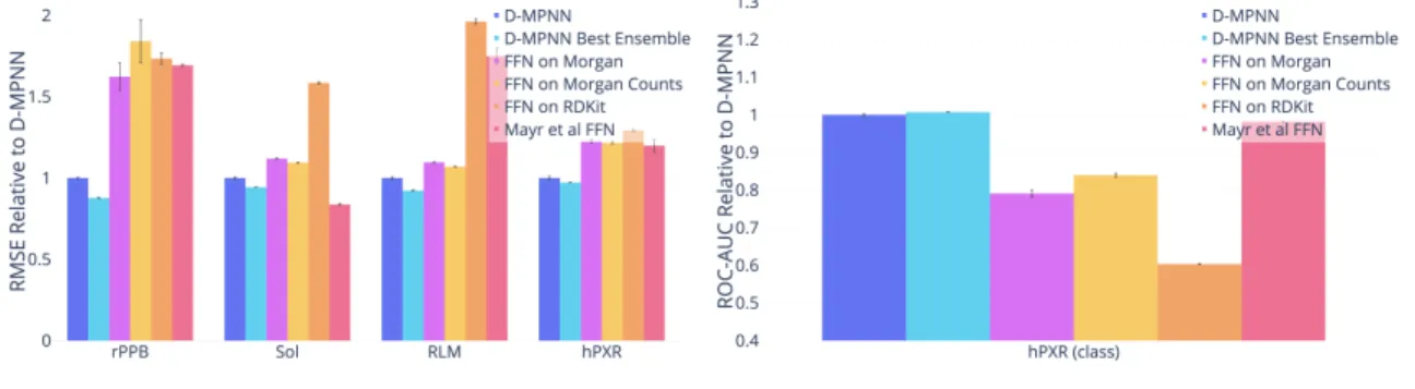
For each dataset, I evaluate on a chronological split. My model significantly outperforms the baselines in almost all cases, as shown in Figure 4-1. Thus my D-MPNN’s strong performance on scaffold splits of public datasets can translate well to chronological splits of private industry datasets.

4.2

BASF

I ran my model on 10 highly related quantum mechanical datasets from BASF. Each dataset contains 13 properties calculated on the same 30,733 molecules, varying the solvent in each dataset. Dataset details are in Table 4.2.

(a) Regression Datasets (lower = better). (b) Classification Datasets (higher = better).

Figure 4-1: Comparison of my D-MPNN against baseline models on Amgen internal datasets on a chronological data split.

For these datasets, I used a scaffold-based split because a chronological split was unavailable. I found that the model of [37] is numerically unstable on these datasets, and I therefore omit it from the comparison below. Once again I find that my model, originally designed to succeed on a wide range of public datasets, is robust enough to transfer to proprietary datasets: D-MPNN models significantly outperform my other baselines, as shown in Figure 4-2.

Category Dataset Tasks Task Type # Compounds Metric Quantum Mechanics Benzene 13 regression 30,733 R2

Quantum Mechanics Cyclohexane 13 regression 30,733 R2

Quantum Mechanics Dichloromethane 13 regression 30,733 R2 Quantum Mechanics DMSO 13 regression 30,733 R2

Quantum Mechanics Ethanol 13 regression 30,733 R2

Quantum Mechanics Ethyl acetate 13 regression 30,733 R2

Quantum Mechanics H2O 13 regression 30,733 R2

Quantum Mechanics Octanol 13 regression 30,733 R2

Quantum Mechanics Tetrahydrofuran 13 regression 30,733 R2

Quantum Mechanics Toluene 13 regression 30,733 R2

Table 4.2: Details on internal BASF datasets. Note: R2 _{is the square of Pearson’s}

4.3

Novartis

Finally, I ran my model on one proprietary dataset from Novartis as described in Table 4.3. I use chronological splits for both datasets. Again I found the model of [37] to be unstable on these datasets, so it is omitted from comparisons. As with other proprietary datasets, my D-MPNN outperforms the other baselines as shown in Figure 4-3.

Figure 4-2: Comparison of my D-MPNN against baseline models on BASF internal regression datasets on a chronological data split (higher = better).

4.4

Experimental Error

As a final “oracle” baseline, I compare my model’s performance with to an experi-mental upper upper bound: the agreement between multiple runs of the same assay, which I refer to as the experimental error. Figure 4-4 shows the R2 _{of my model}

on the private Amgen regression datasets together with the experimental error; in addition, this graph shows the performance of Amgen’s internal model using expert-crafted descriptors. Although my D-MPNN outperforms the Amgen internal model on all but the smallest rPPB dataset, both models remain far less accurate than the corresponding ground truth assays. Thus there remains significant space for further performance improvement in the future.

Category Dataset Tasks Task Type # Compounds Metric

Physical Chemistry logP 1 regression 20,294 RMSE

Figure 4-3: Comparison of my D-MPNN against baseline models on the Novartis internal regression dataset on a chronological data split (lower = better).

Figure 4-4: Comparison of Amgen’s internal model and my D-MPNN (evaluated on a chronological split) to experimental error (higher = better). Note that the experimental error is not evaluated on the exact same time split as the two models since it can only be measured on molecules which were tested more than once, but even so the difference in performance is striking.

Chapter 5

Analysis of Split Type

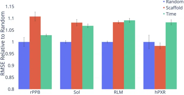
I now justify my use of scaffold splits for performance evaluation. The ultimate goal of building a property prediction model is to predict properties on new chemistry in order to aid the search for drugs from new classes of molecules. On proprietary company datasets, performance on new chemistry is evaluated using a chronological split of the data, i.e., everything before a certain date serves as the training set while everything after that date serves as the test set. This approximates model performance on molecules that chemists are likely to investigate in the future. Since chronological data is typically unavailable for public datasets, I investigate whether I can use my scaffold split as a reasonable proxy for a chronological split.

Figure 5-1 provides motivation for a scaffold split approach. As illustrated in the figure, train and test sets according to a chronological split share significantly fewer molecular scaffolds than train and test sets split randomly. Since my scaffold split enforces zero molecular scaffold overlap between the train and test set, it should ideally provide a split that is at least as difficult as a chronological split.

As illustrated in Figures 5-2, 5-3, and 5-4, performance on my scaffold split is on average closer to performance on a chronological split on proprietary datasets from Amgen and Novartis and on the public PDBBind datasets. However, results are noisy due to the nature of chronological splitting, where I only have a single data split (as opposed to random and scaffold splitting, which both have a random component and can generate different splits depending on the random seed). Figure

5-5 shows the difference between a random split and a scaffold split on the publicly available datasets, further demonstrating that a scaffold split generally results in a more difficult, and ideally more useful, measure of performance. Therefore, all of my results are reported on a scaffold split in order to better reflect the generalization ability of my model on new chemistry.

Figure 5-1: Overlap of molecular scaffolds between the train and test sets for a random or chronological split of four Amgen regression datasets. Overlap is defined as the percent of molecules in the test set which share a scaffold with a molecule in the train set.

Figure 5-2: Performance of D-MPNN on four Amgen regression datasets according to three methods of splitting the data (lower = better).

Figure 5-3: Performance of D-MPNN on the Novartis regression dataset according to three methods of splitting the data (lower = better).

Figure 5-4: Performance of D-MPNN on the full (F), core (C), and refined (R) subsets of the PDBBind dataset according to three methods of splitting the data (lower = better).

(a) Regression Datasets (lower = better). (b) Classification Datasets (higher = better).

Figure 5-5: Performance of D-MPNN on random and scaffold splits for several public datasets.

Chapter 6

Molecular Generation

In this chapter I discuss my efforts in extending our chemical property prediction model for use in the molecular generation space. My first foray into this area was in collaboration with Wengong Jin. In [25] I implemented a molecular generation baseline model operating on SMILES strings, outperforming several previous state-of-the-art methods. Next, I discuss my attempts to build upon this model using reinforcement learning and self-training, and present some preliminary results.

6.1

A Translation Approach to Molecular

Genera-tion

In addition to property prediction, lead optimization is a common real-world set-ting in drug discovery where machine learning tools show great promise. In lead optimization, medicinal chemists already have a candidate molecule with promising properties, and the task is to modify the candidate molecule, or lead, in such a way as to improve upon those properties before beginning additional expensive experiments and/or clinical trials. In the machine learning parlance, I will refer to this task as con-ditional molecular generation. This is because the optimization task is conditioned upon having a particular source molecule, in contrast to approaches like [41] which solve an unconditional optimization task in which they simply generate a library of

molecules with desirable property scores.

Following Jin’s suggestions, I implemented a conditional molecular generation model operating on SMILES strings inspired by existing translation approaches from natural language processing. I tested this model on four datasets; details are given in [25]. The format of each dataset is a series of (source, target) pairs, where each target is a molecule similar to the source (defined by some Tanimoto similarity threshold) with improved property score. Each dataset optimizes a particular computed prop-erty, and defines success by a property range for the translation as well as a similarity threshold for the translation compared to the original input molecule. Furthermore, following [25], during translation I translate each source molecule 20 times, and use success rate and diversity of generated translations as defined in [25] as my main metrics.

6.1.1

Methods and Neural Architecture

My model, also described in [25] operates on an input SMILES string representation of a molecule using a modified character-based translation approach borrowed from natural language processing. I run a single-layer bidirectional LSTM [22] on the character embeddings of the individual characters within the input SMILES string to obtain encoder outputs at each position of the LSTM. The LSTM uses a 300-dimensional hidden state. Then a unidirectional LSTM decoder, augmented with attention [3], decodes character-by-character, trained using teacher forcing at each generation step to arrive at the target SMILES.

In addition, during training, I augment these encodings with an 8-dimensional encoding of the target molecule. In particular, I reuse the encoder LSTM on the target molecule, and then compress the resulting representation to an 8-dimensional mean and log-variance for use as variational noise. The resulting sample from variational noise is appended to each of the encoder output states from the source encoding. As a result, during training, the decoder learns to rely upon this noise to inform it of the structure the target. During testing, when we sample this noise randomly from a Gaussian prior, this results in significantly improved diversity of generated

Figure 6-1: Table from [25] containing results of baselines and my model as well as a stronger graph-based model.

translations. This also corresponds to a higher success rate, as in a more diverse set of translations it is more likely for at least one to be successful.

The resulting SMILES-to-SMILES baseline underperforms a stronger graph-based model of a similar nature that also uses a generative adversarial network to improve its decoder. However, it significantly improves upon the conditional generation per-formance of many prior models, as shown in Figure 6-1.

6.2

Augmentation by Reinforcement Learning

I next attempted to improve the performance of my conditional molecular generation model using deep reinforcement learning [38], although this attempt was ultimately unsuccessful. I set up a gym [1] environment for SMILES generation, in which the action space was the set of allowable characters in a SMILES string, including a special end-of-string token which terminated the episode. The resulting SMILES string was taken as the concatenation of all previously generated characters, and the final reward was the property score of the SMILES string, or some negative penalty when the SMILES string was invalid. I did not give the model intermediate rewards. I tested this method on the logp property because it is easily computable in RDKit [31].

translat-ing it to PyTorch where appropriate. In particular, I used the vanilla policy gradient and proximal policy optimization methods, as these methods have implementations for discrete environments in spinup.

Ultimately, I found that neither method was capable of even learning SMILES syntax when the reward signal was only given at the end of molecule generation, and thus abandoned the reinforcement learning approach. Even when the proximal policy optimization method eventually converged to a solution in which it was capable of generating valid SMILES most of the time, upon inspection I discovered that it had learned simply to generate the string “CâĂİ corresponding to methane. Consistent with the reinforcement learning literature, it appears that more intermediate reward signals were necessary for stable learning [38], but it was unclear how to incorporate such reward signals in this molecule generation setting. Perhaps one could learn a model to predict the eventual property score of a molecule with a given prefix.

6.3

Augmentation by Self Training

Lastly, I implemented a self-training approach for augmenting the performance of the SMILES-to-SMILES molecular generation model, following ideas arising from discussion with Professor Tommi Jaakkola. I conducted experiments on the QED dataset and discuss some preliminary results.

For this approach, I trained my baseline model for several epochs on the QED dataset to reach a reasonable initial level of performance before beginning a self-training loop. After some experimentation and discussion with Professor Jaakkola, I settled on the following methodology. First, for each source molecule in the training set, I translate it 200 times using the existing model, and use the property score evaluator to pick out 4 unique successful translations (for source molecules with less than 4 unique successful translations I simply reuse the target translation given in the training dataset). This increases the total number of training pairs in the training dataset fivefold, although the number of source molecules did not increase.

performance on the QED drug-likeness dataset. Prior to the self-training, I achieved a success rate of 52% (parameters were not exactly matched with the reference baseline from [25] compared to 61% following self-training on the test set. This success rate actually matches that of the stronger graph-based generation model from [25], and the diversity has improved compared to the original baseline as well.

Following this success, I am continuing to explore further improvements to the model performance by investigating different variants of this self training approach. Furthermore, I am applying this model for conditional molecular generation to the task of optimizing for antibiotic potency, for an ongoing project in collaboration with Jonathan Stokes at the Broad Institute. Using growth inhibition data for pseu-domonas aeruginosa, I trained a property predictor for pseupseu-domonas growth inhibi-tion. I am now applying this self training method with the goal of optimizing the inhi-bition potential of the molecule SU 3327, a promising molecule which we have found to have strong antibiotic activity against a wide range of other antibiotic-resistant bacteria, but not pseudomonas aeruginosa.

Chapter 7

Conclusions and Further Work

In this thesis, I have described a novel message-passing based graph convolutional net-work for molecular property prediction. My approach, developed together with Kyle Swanson, significantly improves over strong state-of-the-art baselines such as [50] and [37]. I show that this new message passing algorithm continues to perform strongly on proprietary real-world datasets, using the more realistic chronological splits where available and using scaffold-based approximations to the chronological split other-wise. This conclusion holds on myriad and varied property prediction datasets from Amgen, BASF, and Novartis. Our results have important real-world applications to screening in drug discovery. In fact, our model is already being applied to screen-ing for antibiotic potency in a project in collaboration with the Broad Institute at MIT [48]. Finally, I demonstrate promising innovations for the field of molecular gen-eration, combining translation-based approaches with self training ideas to achieve strong preliminary results.

There remains a great deal of room for further exploration in both property pre-diction and molecular generation. In property prepre-diction, our models still fall short of experimental assay accuracy, and in molecular generation, our success rates for molecule translation remain far from perfect. Ideas for future exploration into in-cludes additional forays into pretraining-based approaches, as described by Swanson in [48], as well as investigating model architectures that more effectively take advan-tage of 3D information and structures. For molecular generation, it is likely that using

a graph-based model such as those described in [25] would lend a useful inductive bias that could further improve the results in this thesis.

Appendix A

Additional Tables and Graphs

A.1

Amgen

Comparison of my D-MPNN in both its unoptimized and optimized form against baseline models on Amgen internal datasets using a time split of the data. Note: The model was optimized on a random split of the data but evaluated on a time split of the data. Also, note that rPPB is in logit while Sol and RLM are in log₁₀.

Dataset D-MPNN D-MPNN Best Ensemble FFN on Morgan rPPB 1.063 ± 0.014 0.933 ± 0.011 (-12.23%) 1.726 ± 0.282 (+62.33%)

Sol 0.710 ± 0.016 0.670 ± 0.002 (-5.61%) 0.794 ± 0.009 (+11.95%) RLM 0.328 ± 0.008 0.303 ± 0.003 (-7.70%) 0.360 ± 0.004 (+9.65%) hPXR 36.789 ± 1.164 35.761 ± 0.168 (-2.79%) 45.113 ± 1.201 (+22.63%) hPXR (class) 0.841 ± 0.008 0.848 ± 0.002 (+0.74%) 0.666 ± 0.024 (-20.90%)

Table A.1: Comparison to Baselines on Amgen, Part I. Note: The metric for hPXR (class) is ROC-AUC; all others are RMSE.

(a) Regression Datasets (lower = better). (b) Classification Datasets (higher = better).

Dataset FFN on Morgan Counts FFN on RDKit Mayr et al.[37] rPPB 1.957 ± 0.444 (+84.14%) 1.844 ± 0.118 (+73.46%) 1.800 ± 0.023 (+69.33%) Sol 0.777 ± 0.005 (+9.45%) 1.125 ± 0.014 (+58.54%) 0.594 ± 0.017 (-16.28%) RLM 0.351 ± 0.003 (+6.97%) 0.644 ± 0.017 (+96.20%) 0.574 ± 0.052 (+74.94%) hPXR 44.753 ± 0.774 (+21.65%) 47.574 ± 0.881 (+29.32%) 44.100 ± 4.590 (+19.87%) hPXR (class) 0.706 ± 0.014 (-16.03%) 0.508 ± 0.003 (-39.66%) 0.826 ± 0.002 (-1.82%)

Table A.2: Comparison to Baselines on Amgen, Part II. Note: The metric for hPXR (class) is ROC-AUC; all others are MSE.

A.2

Amgen Model Optimizations

Dataset

D-MPNN

D-MPNN Optimized

rPPB

1.063 ± 0.014

1.104 ± 0.109 (+3.88%)

Sol

0.710 ± 0.016

0.696 ± 0.018 (-1.89%)

RLM

0.328 ± 0.008

0.320 ± 0.006 (-2.40%)

hPXR

36.789 ± 1.164

37.904 ± 0.920 (+3.03%)

hPXR (class)

0.841 ± 0.008

0.833 ± 0.007 (-1.00%)

Table A.3: Optimizations on Amgen, Part I. Note: The metric for hPXR (class) is ROC-AUC; all others are RMSE.

(a) Regression Datasets (lower = better). (b) Classification Datasets (higher = better).

Dataset D-MPNN Optimized + Features D-MPNN Best Ensemble rPPB 0.964 ± 0.029 (-9.33%) 0.933 ± 0.011 (-12.23%) Sol 0.686 ± 0.008 (-3.25%) 0.670 ± 0.002 (-5.61%) RLM 0.317 ± 0.006 (-3.48%) 0.303 ± 0.003 (-7.70%) hPXR 36.751 ± 0.894 (-0.10%) 35.761 ± 0.168 (-2.79%) hPXR (class) 0.837 ± 0.006 (-0.55%) 0.848 ± 0.002 (+0.74%) Table A.4: Optimizations on Amgen, Part II. Note: The metric for hPXR (class) is ROC-AUC; all others are RMSE.

Dataset Depth Dropout FFN Layers Hidden Size Parameters

rPPB 5 0.1 2 1300 4,135,901

Sol 3 0.05 3 1800 7,617,303

RLM 4 0.1 2 1000 2,581,601

hPXR 2 0.15 3 2200 11,049,402

hPXR (class) 3 0.1 3 600 1,159,802

Table A.5: Optimal Hyperparameter Settings on Amgen.

Dataset Features? rPPB Yes Sol Yes RLM Yes hPXR Yes hPXR (class) Yes

Table A.6: Whether RDKit features improve D-MPNN performance on Amgen datasets.

A.3

BASF

Comparison of my D-MPNN in both its unoptimized and optimized form against baseline models on BASF internal datasets using a scaffold split of the data. Note: The model was optimized on a random split of the data but evaluated on a scaffold split of the data.

Figure A-3: Comparison to Baselines on BASF (higher = better).

Dataset D-MPNN D-MPNN Best Ensemble FFN on Morgan Benzene 0.810 ± 0.011 0.849 ± 0.011 (+4.85%) 0.610 ± 0.017 (-24.68%) Cyclohexane 0.758 ± 0.009 0.792 ± 0.008 (+4.55%) 0.510 ± 0.020 (-32.65%) Dichloromethane 0.813 ± 0.012 0.843 ± 0.014 (+3.72%) -0.030 ± 0.218 (-103.74%) DMSO 0.829 ± 0.009 0.875 ± 0.008 (+5.45%) 0.582 ± 0.019 (-29.77%) Ethanol 0.823 ± 0.008 0.858 ± 0.003 (+4.25%) 0.578 ± 0.020 (-29.80%) Ethyl acetate 0.828 ± 0.008 0.866 ± 0.008 (+4.62%) 0.562 ± 0.024 (-32.05%) H2O 0.821 ± 0.009 0.867 ± 0.008 (+5.65%) 0.575 ± 0.019 (-30.01%) Octanol 0.825 ± 0.008 0.859 ± 0.007 (+4.08%) 0.571 ± 0.017 (-30.84%) Tetrahydrofuran 0.829 ± 0.008 0.868 ± 0.007 (+4.74%) 0.565 ± 0.018 (-31.85%) Toluene 0.826 ± 0.012 0.862 ± 0.011 (+4.36%) 0.562 ± 0.022 (-32.01%)

Dataset FFN on Morgan Counts FFN on RDKit Benzene 0.564 ± 0.021 (-30.40%) 0.734 ± 0.014 (-9.39%) Cyclohexane 0.557 ± 0.017 (-26.44%) 0.677 ± 0.012 (-10.60%) Dichloromethane -0.120 ± 0.306 (-114.82%) 0.671 ± 0.026 (-17.46%) DMSO 0.632 ± 0.020 (-23.83%) 0.751 ± 0.012 (-9.43%) Ethanol 0.628 ± 0.015 (-23.76%) 0.746 ± 0.012 (-9.33%) Ethyl acetate 0.611 ± 0.017 (-26.19%) 0.743 ± 0.012 (-10.17%) H2O 0.626 ± 0.018 (-23.79%) 0.745 ± 0.012 (-9.28%) Octanol 0.622 ± 0.018 (-24.58%) 0.745 ± 0.011 (-9.73%) Tetrahydrofuran 0.610 ± 0.016 (-26.45%) 0.742 ± 0.012 (-10.51%) Toluene 0.605 ± 0.023 (-26.73%) 0.748 ± 0.013 (-9.42%) Table A.8: Comparison to Baselines on BASF, Part II. Note: All numbers are R2.

A.4

BASF Model Optimization

Dataset D-MPNN D-MPNN Optimized Benzene 0.810 ± 0.011 0.828 ± 0.010 (+2.18%) Cyclohexane 0.758 ± 0.009 0.780 ± 0.009 (+2.92%) Dichloromethane 0.813 ± 0.012 0.819 ± 0.011 (+0.76%) DMSO 0.829 ± 0.009 0.856 ± 0.008 (+3.18%) Ethanol 0.823 ± 0.008 0.852 ± 0.008 (+3.55%) Ethyl acetate 0.828 ± 0.008 0.848 ± 0.010 (+2.52%) H2O 0.821 ± 0.009 0.850 ± 0.007 (+3.52%) Octanol 0.825 ± 0.008 0.840 ± 0.007 (+1.84%) Tetrahydrofuran 0.829 ± 0.008 0.848 ± 0.007 (+2.33%) Toluene 0.826 ± 0.012 0.848 ± 0.013 (+2.63%) Table A.9: Optimizations on BASF, Part I. Note: All numbers are R2_.

Dataset D-MPNN Optimized + Features D-MPNN Best Ensemble Benzene 0.840 ± 0.011 (+3.69%) 0.849 ± 0.011 (+4.85%) Cyclohexane 0.786 ± 0.008 (+3.77%) 0.792 ± 0.008 (+4.55%) Dichloromethane 0.829 ± 0.013 (+2.02%) 0.843 ± 0.014 (+3.72%) DMSO 0.862 ± 0.009 (+3.93%) 0.875 ± 0.008 (+5.45%) Ethanol 0.844 ± 0.009 (+2.54%) 0.858 ± 0.003 (+4.25%) Ethyl acetate 0.859 ± 0.008 (+3.78%) 0.866 ± 0.008 (+4.62%) H2O 0.857 ± 0.009 (+4.36%) 0.867 ± 0.008 (+5.65%) Octanol 0.852 ± 0.009 (+3.32%) 0.859 ± 0.007 (+4.08%) Tetrahydrofuran 0.859 ± 0.008 (+3.58%) 0.868 ± 0.007 (+4.74%) Toluene 0.853 ± 0.011 (+3.24%) 0.862 ± 0.011 (+4.36%)

Figure A-4: Optimizations on BASF (higher = better).

Dataset Depth Dropout FFN Layers Hidden Size Parameters

Benzene 5 0.05 2 500 897,513 Cyclohexane 6 0.2 3 1400 8,254,413 Dichloromethane 2 0 2 1100 3,954,513 DMSO 6 0.05 2 1700 9,171,513 Ethanol 6 0.4 2 2400 17,988,013 Ethyl acetate 5 0.1 2 700 1,676,513 H2O 6 0.1 3 1900 15,002,413 Octanol 3 0.25 3 1300 7,144,813 Tetrahydrofuran 4 0.1 3 1200 6,115,213 Toluene 5 0.1 3 1300 7,144,813

Dataset Features? Benzene Yes Cyclohexane Yes Dichloromethane Yes DMSO Yes Ethanol No

Ethyl acetate Yes

H2O Yes

Octanol Yes

Tetrahydrofuran Yes

Toluene Yes

Table A.12: Whether RDKit features improve D-MPNN performance on BASF datasets.

A.5

Novartis

Comparison of my D-MPNN in both its unoptimized and optimized form against baseline models on a Novartis internal dataset using a time split of the data. Note: The model was optimized on a random split of the data but evaluated on a time split of the data.

Dataset D-MPNN D-MPNN Best Ensemble FFN on Morgan

logP 0.674 ± 0.010 0.585 ± 0.004 (-13.17%) 0.887 ± 0.035 (+31.56%) Table A.13: Comparison to Baselines on Novartis, Part I. Note: All numbers are RMSE.

Dataset FFN on Morgan Counts FFN on RDKit logP 0.812 ± 0.016 (+20.52%) 0.730 ± 0.007 (+8.38%)

Table A.14: Comparison to Baselines on Novartis, Part II. Note: All numbers are RMSE.

Figure A-5: Comparison to Baselines on Novartis (lower = better).

A.6

Novartis Model Optimizations

Dataset D-MPNN D-MPNN Optimized

logP 0.674 ± 0.010 0.668 ± 0.022 (-0.94%)

Table A.15: Optimizations on Novartis, Part I. Note: All numbers are RMSE.

Dataset D-MPNN Optimized + Features D-MPNN Best Ensemble

logP 0.607 ± 0.014 (-9.88%) 0.585 ± 0.004 (-13.17%)

Table A.16: Optimizations on Novartis, Part II. Note: All numbers are RMSE.

Dataset Depth Dropout FFN Layers Hidden Size Parameters

logP 5 0.05 3 600 1,610,401

Table A.17: Optimal Hyperparameter Settings on Novartis.

Dataset Features?

logP Yes

Table A.18: Whether RDKit features improve D-MPNN performance on the Novartis dataset.

Figure A-6: Optimizations on Novartis (lower = better).

A.7

Additional Novartis Results

I provide additional results for different versions of my D-MPNN model as well as for a Lasso regression model[20] on the Novartis dataset in Figures 7, 8, and A-9. These results showcase the importance of proper normalization for the additional RDKit features. My base D-MPNN predicts a logP within 0.3 of the ground truth on 47.4% of the test set, comparable to the best Lasso baseline. However, augmenting my model with features normalized using a Gaussian distribution assumption (simply subtracting the mean and dividing by the standard deviation for each feature) results in only 43.0% of test set predictions within 0.3 of the ground truth. But using properly normalized CDFs drastically improves this number to 51.2%. Note that the Lasso baseline runs on Morgan fingerprints as well as RDKit features using properly normalized CDFs.

(a) Binned distribution of errors for Lasso baseline.

(b) Scatterplot of Lasso baseline predictions vs. ground truth.

Figure A-7: Performance of Lasso models on the proprietary Novartis logP dataset. For each model, a pie chart shows the binned distribution of errors on the test set, and a scatterplot shows the predictions vs. ground truth for individual data points.

(a) Binned distribution of errors for D-MPNN.

(b) Scatterplot of predictions vs. ground truth for D-MPNN.

Figure A-8: Performance of base D-MPNN model on the proprietary Novartis logP dataset. A pie chart shows the binned distribution of errors on the test set, and a scatterplot shows the predictions vs. ground truth for individual data points.

(a) Binned distribution of errors for D-MPNN with features normalized according to a Gaussian distribution assumption.

(b) Scatterplot of predictions vs. ground truth for D-MPNN with features normal-ized according to a Gaussian distribution assumption.

(c) Binned distribution of errors for D-MPNN with features normalized using CDFs.

(d) Scatterplot of predictions vs. ground truth for D-MPNN with features normal-ized using CDFs.

Figure A-9: Performance of D-MPNN models with features on proprietary Novartis logP dataset. For each model, a pie chart shows the binned distribution of errors on the test set, and a scatterplot shows the predictions vs. ground truth for individual data points.

A.8

Experimental Error

Comparison of Amgen’s internal model and my D-MPNN (evaluated on a chronolog-ical split) to experimental error. Note that the experimental error is not evaluated on the exact same time split as the two models since it can only be measured on molecules which were tested more than once, but even so the difference in perfor-mance is striking.

Figure A-10: Experimental Error on Amgen (higher = better).

Dataset Amgen D-MPNN Best Experimental

rPPB 0.56 0.55 0.736 RLM 0.53 0.59 0.848 Sol HCL 0.63 0.71 0.782 Sol PBS 0.64 0.69 0.856 Sol SIF 0.24 0.28 0.614 hPXR 2uM 0.24 0.3 0.579 hPXR 10uM 0.33 0.34 0.668

A.9

Analysis of Split Type

Figure A-11: Overlap of molecular scaffolds between the train and test sets for a random or chronological split of four Amgen regression datasets. Overlap is defined as the percent of molecules in the test set which share a scaffold with a molecule in the train set.

Dataset Random Time

rPPB 67.74% 47.84%

Sol 69.31% 33.07%

RLM 75.45% 21.32%

hPXR 79.12% 34.14%

Table A.20: Overlap of molecular scaffolds between the train and test sets for a random or chronological split of four Amgen regression datasets. Overlap is defined as the percent of molecules in the test set which share a scaffold with a molecule in the train set.

Figure A-12: D-MPNN Performance by Split Type on Amgen datasets (lower = better).

Dataset Random Scaffold Time

rPPB 1.033 ± 0.062 1.145 ± 0.063 (+10.78%) 1.063 ± 0.014 (+2.89%) Sol 0.664 ± 0.012 0.718 ± 0.029 (+8.20%) 0.710 ± 0.016 (+6.85%) RLM 0.301 ± 0.004 0.326 ± 0.006 (+8.37%) 0.328 ± 0.008 (+9.16%) hPXR 33.969 ± 3.107 33.401 ± 1.354 (-1.67%) 36.789 ± 1.164 (+8.30%) Table A.21: D-MPNN Performance by Split Type on Amgen datasets. Note: All numbers are RMSE.

Figure A-13: D-MPNN Performance by Split Type on Novartis datasets (lower = better).

Dataset Random Scaffold Time

logP 0.540 ± 0.027 0.557 ± 0.034 (+3.07%) 0.674 ± 0.010 (+24.80%) Table A.22: Performance of D-MPNN on different data splits on Novartis datasets. Note: All numbers are RMSE.

Dataset Random Scaffold Time

PDBbind-F 1.264 ± 0.026 1.347 ± 0.028 (+6.56%) 1.390 ± 0.017 (+9.96%) PDBbind-C 1.910 ± 0.137 2.047 ± 0.244 (+7.20%) 2.160 ± 0.080 (+13.11%) PDBbind-R 1.318 ± 0.063 1.413 ± 0.057 (+7.19%) 1.530 ± 0.018 (+16.10%) Table A.23: D-MPNN Performance by Split Type on PDBBind. Note: All numbers are RMSE.

(a) Regression Datasets (lower = better). (b) Classification Datasets (higher = better).

Figure A-15: D-MPNN Performance by Split Type on Public Datasets.

Dataset Metric Random Scaffold

QM7 MAE 67.657 ± 3.647 102.302 ± 7.532 (+51.21%) QM8 MAE 0.0111 ± 0.0001 0.0148 ± 0.0019 (+33.49%) QM9 MAE 3.705 ± 0.537 5.177 ± 1.848 (+39.72%) ESOL RMSE 0.691 ± 0.080 0.862 ± 0.094 (+24.77%) FreeSolv RMSE 1.133 ± 0.176 1.932 ± 0.412 (+70.49%) Lipophilicity RMSE 0.598 ± 0.064 0.656 ± 0.047 (+9.79%) PDBbind-F RMSE 1.325 ± 0.027 1.374 ± 0.028 (+3.70%) PDBbind-C RMSE 2.088 ± 0.194 2.154 ± 0.290 (+3.12%) PDBbind-R RMSE 1.411 ± 0.060 1.468 ± 0.075 (+4.00%) PCBA PRC-AUC 0.329 ± 0.007 0.271 ± 0.011 (-17.56%) MUV PRC-AUC 0.0865 ± 0.0456 0.0807 ± 0.0494 (-6.76%) HIV ROC-AUC 0.811 ± 0.037 0.782 ± 0.016 (-3.52%) BACE ROC-AUC 0.863 ± 0.028 0.825 ± 0.039 (-4.40%) BBBP ROC-AUC 0.920 ± 0.017 0.915 ± 0.037 (-0.52%) Tox21 ROC-AUC 0.847 ± 0.012 0.808 ± 0.025 (-4.57%) ToxCast ROC-AUC 0.735 ± 0.014 0.690 ± 0.011 (-6.04%) SIDER ROC-AUC 0.639 ± 0.024 0.606 ± 0.029 (-5.23%) ClinTox ROC-AUC 0.892 ± 0.043 0.874 ± 0.041 (-2.00%) ChEMBL ROC-AUC 0.745 ± 0.031 0.709 ± 0.010 (-4.81%) Table A.24: D-MPNN Performance by Split Type on Public Datasets.

Bibliography

[1] https://gym.openai.com/.

[2] https://github.com/openai/spinningup.

[3] Dzmitry Bahdanau, Kyunghyun Cho, and Yoshua Bengio. Neural machine trans-lation by jointly learning to align and translate. arXiv preprint arXiv:1409.0473, 2014.

[4] Peter Battaglia, Razvan Pascanu, Matthew Lai, and Danilo Jimenez Rezende. Interaction networks for learning about objects, relations and physics. Advances in Neural Information Processing Systems, pages 4502–4510, 2016.

[5] Leo Breiman. Random forests. Machine learning, 45(1):5–32, 2001.

[6] Joan Bruna, Wojciech Zaremba, Arthur Szlam, and Yann LeCun. Spectral net-works and locally connected netnet-works on graphs. arXiv preprint arXiv:1312.6203, 2013.

[7] Dong-Sheng Cao, Qing-Song Xu, Qian-Nan Hu, and Yi-Zeng Liang. Chemopy: Freely available python package for computational biology and chemoinformatics. Bioinformatics, 29(8):1092–1094, 2013.

[8] Connor W. Coley, Regina Barzilay, William H. Green, Tommi S. Jaakkola, and Klavs F. Jensen. Convolutional embedding of attributed molecular graphs for physical property prediction. Journal of Chemical Information and Modeling, 57(8):1757–1772.

[9] Corinna Cortes and Vladimir Vapnik. Support vector machine. Machine Learn-ing, 20(3):273–297, 1995.

[10] Hanjun Dai, Bo Dai, and Le Song. Discriminative embeddings of latent vari-able models for structured data. International Conference on Machine Learning, pages 2702–2711, 2016.

[11] Michaël Defferrard, Xavier Bresson, and Pierre Vandergheynst. Convolutional neural networks on graphs with fast localized spectral filtering. Advances in Neural Information Processing Systems, pages 3844–3852, 2016.

[12] Thomas G Dietterich. Ensemble methods in machine learning. International Workshop on Multiple Classifier Systems, pages 1–15, 2000.

[13] Joseph L Durant, Burton A Leland, Douglas R Henry, and James G Nourse. Reoptimization of mdl keys for use in drug discovery. Journal of Chemical In-formation and Computer Sciences, 42(6):1273–1280, 2002.

[14] David K Duvenaud, Dougal Maclaurin, Jorge Iparraguirre, Rafael Bombarell, Timothy Hirzel, Alán Aspuru-Guzik, and Ryan P Adams. Convolutional net-works on graphs for learning molecular fingerprints. Advances in Neural Infor-mation Processing Systems, pages 2224–2232, 2015.

[15] Felix A Faber, Luke Hutchison, Bing Huang, Justin Gilmer, Samuel S Schoen-holz, George E Dahl, Oriol Vinyals, Steven Kearnes, Patrick F Riley, and O Ana-tole von Lilienfeld. Machine learning prediction errors better than dft accuracy. arXiv preprint arXiv:1702.05532, 2017.

[16] Evan N Feinberg, Debnil Sur, Zhenqin Wu, Brooke E Husic, Huanghao Mai, Yang Li, Saisai Sun, Jianyi Yang, Bharath Ramsundar, and Vijay S Pande. Potentialnet for molecular property prediction. ACS Central Science, 4(11):1520– 1530, 2018.

[17] Justin Gilmer, Samuel S. Schoenholz, Patrick F. Riley, Oriol Vinyals, and George E. Dahl. Neural message passing for quantum chemistry. Proceedings of the 34th International Conference on Machine Learning, 2017.

[18] Rafael Gómez-Bombarelli, Jennifer N Wei, David Duvenaud, José Miguel Hernández-Lobato, Benjamín Sánchez-Lengeling, Dennis Sheberla, Jorge Aguilera-Iparraguirre, Timothy D Hirzel, Ryan P Adams, and Alán Aspuru-Guzik. Automatic chemical design using a data-driven continuous representation of molecules. ACS Central Science, 4(2):268–276, 2018.

[19] Will Hamilton, Zhitao Ying, and Jure Leskovec. Inductive representation learn-ing on large graphs. Advances in Neural Information Processlearn-ing Systems, pages 1024–1034, 2017.

[20] Chris Hans. Bayesian lasso regression. Biometrika, 96(4):835–845, 2009.

[21] Mikael Henaff, Joan Bruna, and Yann LeCun. Deep convolutional networks on graph-structured data. arXiv preprint arXiv:1506.05163, 2015.

[22] Sepp Hochreiter and Jürgen Schmidhuber. Lstm can solve hard long time lag problems. In Advances in neural information processing systems, pages 473–479, 1997.

[23] Katsuhiko Ishiguro, Shin-ichi Maeda, and Masanori Koyama. Graph warp mod-ule: An auxiliary module for boosting the power of graph neural networks. arXiv preprint arXiv:1902.01020, 2019.

[24] Wengong Jin, Regina Barzilay, and Tommi Jaakkola. Junction tree variational autoencoder for molecular graph generation. arXiv preprint arXiv:1802.04364, 2018.

[25] Wengong Jin, Kevin Yang, Regina Barzilay, and Tommi Jaakkola. Learning mul-timodal graph-to-graph translation for molecular optimization. arXiv preprint arXiv:1812.01070, 2018.

[26] Steven Kearnes, Kevin McCloskey, Marc Berndl, Vijay Pande, and Patrick Ri-ley. Molecular graph convolutions: Moving beyond fingerprints. Journal of Computer-Aided Molecular Design, 30(8):595–608, 2016.

[27] Thomas N Kipf and Max Welling. Semi-supervised classification with graph convolutional networks. arXiv preprint arXiv:1609.02907, 2016.

[28] Daphne Koller, Nir Friedman, and Francis Bach. Probabilistic graphical models: Principles and techniques. MIT Press, 2009.

[29] Risi Kondor, Hy Truong Son, Horace Pan, Brandon Anderson, and Shubhendu Trivedi. Covariant compositional networks for learning graphs. arXiv preprint arXiv:1801.02144, 2018.

[30] Matt J Kusner, Brooks Paige, and José Miguel Hernández-Lobato. Grammar variational autoencoder. arXiv preprint arXiv:1703.01925, 2017.

[31] Greg Landrum. Rdkit: Open-source cheminformatics. 2006. https://rdkit. org/docs/index.html.

[32] Alpha A. Lee, Qingyi Yang, Asser Bassyouni, Christopher R. Butler, Xinjun Hou, Stephen Jenkinson, and David A. Price. Ligand biological activity predicted by cleaning positive and negative chemical correlations. Proceedings of the National Academy of Sciences, 2019.

[33] Tao Lei, Wengong Jin, Regina Barzilay, and Tommi Jaakkola. Deriving neural architectures from sequence and graph kernels. arXiv preprint arXiv:1705.09037, 2017.

[34] Yujia Li, Daniel Tarlow, Marc Brockschmidt, and Richard Zemel. Gated graph sequence neural networks. arXiv preprint arXiv:1511.05493, 2015.

[35] Ke Liu, Xiangyan Sun, Lei Jia, Jun Ma, Haoming Xing, Junqiu Wu, Hua Gao, Yax Sun, Florian Boulnois, and Jie Fan. Chemi-net: A graph convolutional network for accurate drug property prediction. arXiv preprint arXiv:1803.06236, 2018.

[36] Andrea Mauri, Viviana Consonni, Manuela Pavan, and Roberto Todeschini. Dragon software: An easy approach to molecular descriptor calculations. Match, 56(2):237–248, 2006.

[37] Andreas Mayr, Günter Klambauer, Thomas Unterthiner, Marvin Steijaert, Jörg K. Wegner, Hugo Ceulemans, Djork-Arné Clevert, and Sepp Hochreiter. Large-scale comparison of machine learning methods for drug target prediction on chembl. Chemical Science, 9:5441–5451, 2018.

[38] Volodymyr Mnih, Koray Kavukcuoglu, David Silver, Alex Graves, Ioannis Antonoglou, Daan Wierstra, and Martin Riedmiller. Playing atari with deep reinforcement learning. arXiv preprint arXiv:1312.5602, 2013.

[39] Hirotomo Moriwaki, Yu-Shi Tian, Norihito Kawashita, and Tatsuya Takagi. Mor-dred: A molecular descriptor calculator. Journal of Cheminformatics, 10(1):4, 2018.

[40] Vinod Nair and Geoffrey E. Hinton. Rectified linear units improve restricted boltzmann machines. Proceedings of the 27th International Conference on Ma-chine Learning, 2010.

[41] Mariya Popova, Olexandr Isayev, and Alexander Tropsha. Deep reinforcement learning for de novo drug design. Science advances, 4(7):eaap7885, 2018.

[42] David Rogers and Mathew Hahn. Extended-connectivity fingerprints. Journal of chemical information and modeling, 50(5):742–754, 2010.

[43] Franco Scarselli, Marco Gori, Ah Chung Tsoi, Markus Hagenbuchner, and Gabriele Monfardini. The graph neural network model. IEEE Transactions on Neural Networks, 20(1):61–80, 2009.

[44] Kristof Schütt, Pieter-Jan Kindermans, Huziel Enoc Sauceda Felix, Ste-fan Chmiela, Alexandre Tkatchenko, and Klaus-Robert Müller. Schnet: A continuous-filter convolutional neural network for modeling quantum interac-tions. Advances in Neural Information Processing Systems, pages 991–1001, 2017.

[45] Kristof T Schütt, Farhad Arbabzadah, Stefan Chmiela, Klaus R Müller, and Alexandre Tkatchenko. Quantum-chemical insights from deep tensor neural net-works. Nature Communications, 8:13890, 2017.

[46] B. Shahriari, K. Swersky, Z. Wang, R. P. Adams, and N. de Freitas. Taking the human out of the loop: A review of bayesian optimization. Proceedings of the IEEE, 104(1):148–175, Jan 2016.

[47] S Joshua Swamidass, Jonathan Chen, Jocelyne Bruand, Peter Phung, Liva Ralaivola, and Pierre Baldi. Kernels for small molecules and the prediction of mu-tagenicity, toxicity and anti-cancer activity. Bioinformatics, 21(suppl_1):i359– i368, 2005.

[48] Kyle Swanson. Message passing neural networks for molecular property predic-tion. MIT Master’s Thesis, 2019.

[49] David Weininger. Smiles, a chemical language and information system. 1. intro-duction to methodology and encoding rules. Journal of Chemical Information and Computer Sciences, 28(1):31–36, 1988.

[50] Zhenqin Wu, Bharath Ramsundar, EvanÂăN. Feinberg, Joseph Gomes, Caleb Geniesse, Aneesh S. Pappu, Karl Leswing, and Vijay Pande. Moleculenet: A benchmark for molecular machine learning. Chemical Science, 9(2):513âĂŞ530, 2018.

[51] Kevin Yang, Kyle Swanson, Wengong Jin, Connor Coley, Philipp Eiden, Hua Gao, Angel Guzman-Perez, Timothy Hopper, Brian Kelley, Miriam Mathea, et al. Are learned molecular representations ready for prime time? arXiv preprint arXiv:1904.01561, 2019.