HAL Id: hal-01680426
https://hal-univ-rennes1.archives-ouvertes.fr/hal-01680426
Submitted on 17 Jul 2019
HAL is a multi-disciplinary open access
archive for the deposit and dissemination of
sci-entific research documents, whether they are
pub-lished or not. The documents may come from
teaching and research institutions in France or
abroad, or from public or private research centers.
L’archive ouverte pluridisciplinaire HAL, est
destinée au dépôt et à la diffusion de documents
scientifiques de niveau recherche, publiés ou non,
émanant des établissements d’enseignement et de
recherche français ou étrangers, des laboratoires
publics ou privés.
Distributed under a Creative Commons Attribution| 4.0 International License
Reconstruction Based on Low-rank Matrix Completion
Longyu Jiang, Runguo He, Jie Liu, Yang Chen, Jiasong Wu, Huazhong Shu,
Jean-Louis Coatrieux
To cite this version:
Longyu Jiang, Runguo He, Jie Liu, Yang Chen, Jiasong Wu, et al.. Phase-constrained Parallel
Mag-netic Resonance Imaging Reconstruction Based on Low-rank Matrix Completion. IEEE Access, IEEE,
2018, 6, pp.4941-4954. �10.1109/ACCESS.2017.2780921�. �hal-01680426�
Received October 4, 2017, accepted November 20, 2017, date of publication December 7, 2017, date of current version February 28, 2018.
Digital Object Identifier 10.1109/ACCESS.2017.2780921
Phase-Constrained Parallel Magnetic Resonance
Imaging Reconstruction Based on
Low-Rank Matrix Completion
LONGYU JIANG1,2,3, (Member, IEEE), RUNGUO HE1, JIE LIU1,
YANG CHEN 1,2,3, (Member, IEEE), JIASONG WU 1,2,3, (Member, IEEE),
HUAZHONG SHU1,2,3, (Senior Member, IEEE), AND
JEAN-LOUIS COATRIEUX3,4, (Life Fellow, IEEE)
1Laboratory of Image Science and Technology, Southeast University, Nanjing 210096, China
2Key Laboratory of Computer Network and Information Integration, Ministry of Education, Southeast University, Nanjing 210096, China 3Centre de Recherche en Information Biomedicale Sino-Francais, 35000 Rennes, France.
4Laboratoire Traitement du Signal et de l’ Image, Université de Rennes 1, 35042 Cedex-Rennes, France
Corresponding author: Yang Chen ([email protected])
This work was supported in part by the National Natural Science Foundation of China under Grant 61401085, in part by the State Key Laboratory of Acoustics, Chinese Academy of Sciences under Grant SKLA201604, and in part by the Scientific Research
Foundation for the Returned Overseas Chinese Scholars.
ABSTRACT Low-rank matrix completion with phase constraints have been applied to the single-channel magnetic resonance imaging (MRI) reconstruction. In this paper, the reconstruction of sparse parallel imaging with smooth phase in each coil is formulated as the completion of a low-rank data matrix, which is modeled by the k-space neighborhoods and symmetric property of samples. The proposed algorithm is compared with a calibrationless parallel MRI reconstruction method based on both simulation data and real data. The experiment results show the proposed method has better performance in terms of MRI imaging enhancement, scanning time reduction, and denoising capability.
INDEX TERMS Magnetic resonance imaging, low-rank, matrix completion, phase constraint, parallel imaging.
I. INTRODUCTION
Magnetic resonance imaging (MRI) has been widely applied in medical diagnoses. It is utilized to image the anatomy and the physiological processes. It also plays an important role in subsequent treatments, both exclusive application and com-prehensive combination of various radiation therapies. The duration of an MRI exam can cause difficult to the patient. The scan may last from 15 to 60 minutes with ordinary MRI devices, moreover, the patient have to remain com-pletely stationary during the whole process which is diffi-cult when the patient is a child or a baby. The possibility of achieving detailed images in a shorter time will make the procedure more convenient for patients and also reduce queue time for hospitals. Reducing the long time-consuming of Fourier imaging to form an image is achieved by the approaches of reducing the number of data acquisitions, which includes the constrained reconstruction and parallel imaging [1]–[6].
Constrained reconstruction methods have been paid more attention in modern MRI owing to the splendid capability in reduction of data acquisition and artifacts. Constrained methods utilize mathematics tools such as, parametric mod-eling, and a priori information such as, phase constraints, to compensate for the unsampled experimental data in recon-struction process [7]. In such approaches, dependence rela-tionships based on a priori information are utilized to describe the data relativity which enables the reduction of space-sampling quantity. In other words, dependence relationships imply the existence of redundancy that can predict unsam-pled data on the basis of known ones. Phase-constrained reconstruction is one of common constrained methods. It utilizes partial Fourier transform which relies on Fourier symmetry features of images with foreknown phase informa-tion. The LORAKS technique [8] has investigated the phase constraints in a single channel MRI reconstruction and the relationships of phase constraints was discussed in the Partial
VOLUME 6, 2018
2169-3536 2017 IEEE. Translations and content mining are permitted for academic research only.
Fourier reconstruction through data fitting and convolution in k-space [9].
Parallel imaging is another common manipulation to shorten MRI scanning time by utilizing several spatially distributed coils to receive signals simultaneously. Multi-channel received signals provide data redundancy, which makes it possible to achieve proper reconstruction of under-sampling data. An incomplete list of parallel imaging methods which exploit sensitivity information directly or indirectly includes: (1) reconstruction based on explicit coil sensitivity measurements, such as SMASH [10] and SENSE [11]; (2) autocalibration signals (ACSs) acquisition methods, such as GRAPPA [12] and SPIRiT [13].
In recent years, some matrix completion based techniques have been proposed, like PRUNO [14], LARAKS [8] and ALOHA [15]. Super-resolution MRI using finite rate of inno-vation curves [16] and SAKE [17]. SAKE is also a calibra-tionless reconstruction method [17].
There are many benefits when combining the phase con-straint with parallel imaging in a comprehensive method for MRI. Less data acquisition and better reconstruction result are the most two significant advantages. In previous meth-ods, the combination of phase constraint and parallel imag-ing simply respected a certain order, either parallel imagimag-ing followed by phase-constrained reconstruction or the reverse order. In early research, phase constraint, as a criterion to improve phase estimation, is embedded in the parallel imag-ing method, such as POCSENSE [18], TurboSENSE [19], and initial investigation [20], [21]. Although the two pro-cesses were conducted together, the parallel imaging model of all the approaches is based on SENSE, in which computation of sensitivity map with long acquisition time was necessary. A newly proposed algorithm named P-LARAKS [22] consid-ers both linear relationship and phase constraint in the model, however, they are used separately by corresponding to two independent regularization term.
In this paper, a novel method which incorporates phase constraint and calibrationless parallel imaging in a single procedure is proposed. We expand the phase constraint of two-dimensional k-space datasets used in single-channel MRI reconstruction to three-dimensional k-space datasets which enable the parallel imaging reconstruction. In partic-ular, a hypothesis is made first that the underlying mag-netization image of each coil has slowly varying phase. Under this hypothesis, any unsampled k-space sample can be predicted based on a block constructed by the same neighborhood and the k-space symmetry point in each coil. A data matrix is constructed based on multi-channel k-space dataset. It is proved to be a rank-deficient one and further is reconstructed by matrix completion methods. Therefore, the proposed method concentrates on phase-constrained parallel MRI reconstruction by utilizing low-rank matrix completion. Phase-constrained and low-rank (PCLR) are two primary features of the proposed method. In this work, it was found that the proposed PCLR method had better performance in terms of the reconstruction resolution, denoising capability
and even the reduction of data acquisition compared with SAKE.
II. LINEAR DEPENDENT RELATIONSHIPS
In this section, the linear dependent relationships of parallel imaging and phase constraint on the pixels of underlying magnetization image are derived in the first and second parts respectively. In the third part, the two relationships are con-sidered together and combined in a single formula.
A. LINEAR DEPENDENT RELATIONSHIP OF PARALLEL IMAGING
Without loss of generality, the underlying magnetization image of a whole parallel imaging system is denoted by a two-dimensional matrixρ. The individual channel image in the system is denoted byρifor the i-th coil (with N coils in all) and satisfies the following formula:
ρi=Siρ 1 ≤ i N (1)
where Si represents the sensitivity map of the i-th coil. The
multi-channel form of equation1is formulated as:
ρi= ˆSi N X j=1 ˆ SHj ρj= N X j=1 ˆ SiSˆHj ρj= N X j=1 Sijρj (2)
where the subscript H denotes the Hermitian transpose and ˆ
Si=[PNj=1SHj Sj] −1
2Siis the normalization of Si[23]
Let A(x, y) be the entries of an arbitrary two-dimensional matrix A. Siin equation1is a diagonal matrix. Sij=SiSˆHj is
also a diagonal matrix whose t-th diagonal element is denoted by Sij(t, t). Then, equation2can be rewritten in the following
form: ρi(x, y) = N X j=1 Sij(x, x)ρj(x, y) (3)
B. LINEAR DEPENDENT RELATIONSHIP OF PHASE CONSTRAINT
In general, the underlying magnetization imageρ(x, y) con-sists of the magnitude component m(x, y) = |ρ(x, y)| and the phase componentϕ = 6 ρ(x, y), then for each entry of the
image, it can be written as in [8]:
ρi(x, y) = m(x, y)h(x, y) (4)
where h(x, y) = exp(iϕρ(x, y)).
In consideration of parallel imaging situation, the con-jugated expression of the underlying magnetization image for i-th coil can be expressed as:
ρ∗
i(x, y) = mi(x, y)h∗i(x, y) = ρi(x, y)(h∗i(x, y))2 (5)
C. DEPENDENT RELATIONSHIP COMBINING PARALLEL IMAGING AND PHASE CONSTRAINT
Substituting equation3into equation5, we have
ρ∗ i(x, y) = N X j=1 Sij(x, x)(h∗i(x, y))2ρj(x, y) = N X j=1 gij(x, y)ρj(x, y) (6) where gij(x, y) = Sij(x, x)(h∗i(x, y))2
Equation 6 shows a dependent relationship between the conjugation of an entry in a certain channel image and entries of each multi-channel image. Both parallel imaging prop-erty and phase constraint are taken into consideration in this dependent relationship. Let ˜ρ[u, v] be the Fourier transform ofρ(x, y), that is,
˜
ρ[u, v] = F{ρ(x, y)} (7)
where F is the Fourier transform operator, and the paren-theses and brackets are used to discriminate the entries in magnetization image and k-space respectively. The k-space form of equation 6 can be derived by using the conjugate symmetry and the convolution theorem of Fourier transform
˜ ρ∗ i[−u, −v] = N X j=1 X [p,q]∈Z2 ˜ gij[p, q]˜pj[u − p, v − q] (8)
Under the hypothesis that the underlying magnetization image in each coil has slowly varying phase, the truncation of Fourier transform, a common manipulation for discrete situations, is suitable to be applied to equation8 and leads to: ˜ ρ∗ i[−u, −v] − N X j=1 X [p,q]∈3 ˜ gij[p, q]˜pj[u − p, v − q] ≈ 0 (9)
where 3 = Z2[−R,R]×[−R,R] denotes the square truncation neighborhood whose length is 2 × R + 1. The expression in equation9 is approximately equal to zero and the preci-sion depends on the size of truncation neighborhood and the smooth condition of phase.
III. METHOD
The reconstruction procedure is composed of three parts, data matrix construction, low-rank matrix reconstruction, and k-space dataset reconstruction. In the paper, different masks are utilized to present different sparse imaging mode. The imaging mode is the same in each channel when a single mask is chosen. For example, in the experiments, masks with different sampling ratios ranging from 15 % to 40 % are utilized. This introduces ’the sparsity’ we mentioned in this paper.
A. DATA MATRIX CONSTRUCTION
Equation9 shows a linear dependent relationship between a k-space sample and the block constructed by same neigh-borhood of k-space symmetry point on k-space center. This relationship can be further exploited to construct a rank-deficient matrix. Assume that samples in a k-space dataset with L rows and M columns (assuming L and M are even), are indexed by [u, v] ∈ R2[R+1,L−R], let
Dl =[d1l, d l 2, . . . , d l N, D l 1, D l 2, . . . , D l N], l = u − R +(v − R + 1) × (L − 2 × R) (10)
where dil and Dli represent the phase-constrained recon-structed component of k-space sample and the parallel imag-ing one respectively. They are shown as follows:
dil = ˜ρ∗
i[l − 2 × R − u, M − 2 × R − v] (11)
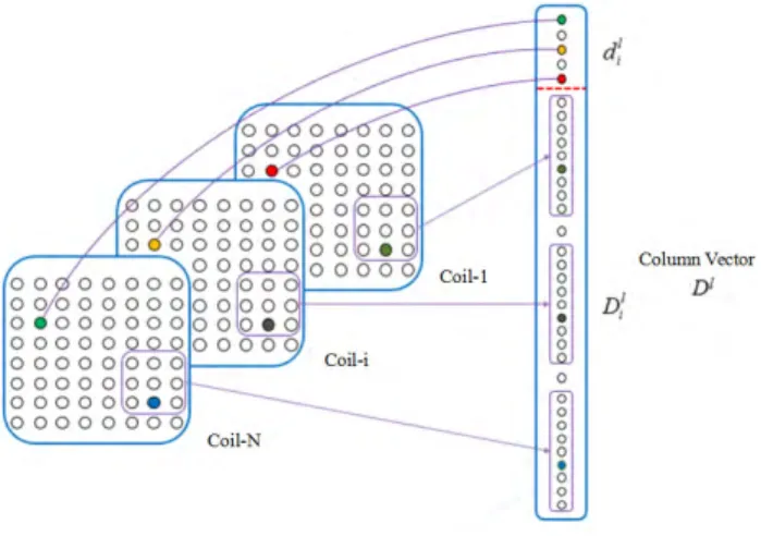
Dil =[ ˜ρli1, ˜ρil2, . . . , ˜ρil(2×R)2+1] (12) with ˜ρilt = ˜ρi[u − p, v−q], t = 2×R2+2 × (q + 1) × R + p + q +1 and (p, q) ∈ Z2[−R,R]×[−R,R]. And the specific manner in which it is constructed is shown in Fig.1.
FIGURE 1. The construction of the column vector Dl. The matrix D is constructed as follows:
D = [D1, D2, . . . , D(L−2×R)(M −2×R)] (13) Data matrix D is composed of column vector Dl and each
Dl is structured based on the linear relationship, equation 9,
which represents a k-space sample is a linear expression of a square neighborhood whose center is symmetry with the aforementioned sample in k-space. Dlcorresponds to the cir-cumstance that the k-space sample index is [−u, −v] and the square neighborhood center index is [u, v]. We traverse the whole k-space in column order and construct data matrix D. Therefore, data matrix D contains all the k-space samples and each column represents a linear expression between a k-space sample and a k-space neighborhood. And the Fig. 2. shows the construction of the Data Matrix D.
Thus, the data matrix D will have a block-wise Hankel structure whose local counter-diagonal entries are the same
FIGURE 2. The construction of the data matrixD.
which can be seen in the Fig.2. A matrix with block Hankel structure possesses the rank-deficiency property [24]. Specif-ically, data matrix D is composed of Dl representing the l-th column vector corresponding to a neighborhood whose center is [u, v] of the k-space dataset. The column vector Dl is composed of two parts, dil and Dli, thus data matrix D can be treated as a row partitioned matrix and represented as
D = [d, D]T (T indicates matrix transpose.), which d and
Drepresent the parts above and below the red dotted line in Fig. 2. According to the property of matrix rank, we have rank(D) ≤ rank(d ) + rank(D). d has N (coil number) rows, therefore, rank(d ) is less than the coil number. Considering D, we should compare Dli and Dl+i 1, which are the reshaped column vectors of the neighborhoods centered on [u, v] and [u + 1, v] based on column arrangement order respectively. Therefore, the local counter-diagonal entries of D are the same k-space samples and such structure is called block-wise Hankel structure. A matrix with block-wise Hankel structure is verified rank-deficient in [23]. Both d and D have a low rank or a deficient rank, the rank of D is obviously low.
The rank of data matrix D is dominantly connected with the truncation neighborhood, as shown in Fig. 3. In equation9, it was shown that the rank to size of truncation neighborhood ratio, termed normalized rank ratio, converges to 1, especially when the size is large as anticipated. In addition, an example illustrating the property is listed as follows.
B. LOW-RANK MATRIX COMPLETION
After the matrix D is constructed, the phase-constrained parallel imaging reconstruction can be transformed into the completion of a structured rank-deficiency matrix. All the known entries in matrix D are assumed to have a support set = {(x, y) ∈ R2: |D(x, y)| 6= 0}. Then, the problem can be
formulated as follows:
minimize rank(X)
subject to X(x, y) = D(x, y), (x, y) ∈ (14)
where X is the estimation of D.
However, the rank minimization is a non-deterministic polynomial-time hard (NP-hard) problem. Fortunately, when the rank of matrix D is known beforehand, a tightest convex
FIGURE 3. A plot that shows how the rank values decay.
relaxation was proposed to simplify the awkward NP-hard problem. It was proved that equation14can be recast into the following convex optimization problem [25], [26].
minimize ||X||∗
subject to rank(X) = r
X(x, y) = D(x, y), (x, y) ∈ (15) where ||X||∗represents the nuclear norm of the matrix X and
it is defined as: ||X||∗= r X i=1 σi (16)
whereσiare the singular values of matrix X, and r is the rank
of matrix X.
In this paper, the classic Cadzow algorithm was selected to solve the problem presented in equation15[17], [27]. The Cadzow algorithm is an iterative method which includes three steps in each single loop:
Step 1: For then-th interation, the singular values matrix 6nof the current estimate of data matrix , Xnis computed by
the singular value decomposition (SVD)
X = Un6nVn (17)
Step 2: The r largest entries of the diagonal of6nare
pre-served to construct the new singular value matrix6n+1with
zero for the other entries. The new estimate of data matrix,
Xn+1, is computed by
X = Un6n+1Vn (18)
Step 3: The estimation Xn+1is subject to the constraint of
data consistency, which is represented as follows:
Xn+1(x, y) = D(x, y), (x, y) ∈ (19)
The iterative procedure stops if the number of iterations reaches a prefixed value or the error is less than a threshold.
FIGURE 4. Variation of SSIM value with different selection ofλ.
C. K-SPACE DATASET RECONSTRUCTION
The k-space dataset needs to be reconstructed after the low-rank data matrix completion. Assume that Ki[u, v] represents
the k-space samples indexed by [u, v] in the i-th channel. Then, reconstruction equation of Ki[u, v] is defined as:
Ki[u, v] = λ × di(L−2×R)×(M −2×R)−l+1 + (1 −λ) (2 × R + 1)2 R X q=−R R X p=−R Dl+p+q×mi (t), t =2 × R2+2 × (q + 1) × R + p + q + 1 (20) where Dli(t) is the t-th entry of Dli.λ, the phase constraint factor, represents the proportion of the two reconstructed components. Once the k-space dataset is reconstructed, the same imaging procedure in E-SPIRiT method [23] and SAKE model is utilized to obtain two-dimensional magne-tization image from multi-channel k-space dataset.
IV. EXPERIMENT AND RESULTS
In this section, both simulation dataset and real dataset are reconstructed by the proposed PCLR method to assess the performance of the method and then to compare to a rel-atively new reconstruction method of parallel MRI, SAKE which showed better reconstruction results than several other methods.
A. EXPERIMENTAL PARAMETERS SELECTION
Structural similarity index measurement (SSIM) compares local patterns of pixel intensities that have been normalized for luminance and contrast [28]. The value of SSIM ranges from 0 to 1 with higher value to represent better reconstruc-tion results. Here the SSIM is used to present the similarity degree between the reconstructed image and the fully sam-pled reconstruction result. Actually in the field of MRI, the images are provided for the doctors, and the structure and contrast of the images are the most important considerations for the diagnosis. Compared with the most widely used image
quality and distortion assessment methods, mean squared error (MSE) and peak signal-to-noise ratio (PSNR) which often do not correlate well with perceived quality, the algo-rithm SSIM which takes the image luminance, contrast and structure into account [29], [30], shows better image quality assessment for the MRI images. In the experiment, each local patch to be tested for similarity is an 11 × 11 Gaussian window. The SSIM index formula K is chosen as K1=0.03
and K2=0.01 for the computation of luminance comparison
and contrast comparison respectively. All the programs were run on a computer with an Intel i5-2400, 3.10GHz CPU and 12GB of memory. In each reconstruction experiment, in order to record the time of calculation which is used to compare the reconstruction speed, 100 times iteration was implemented.
Fig. 4 shows the variation of SSIM value between recon-struction result and fully sampled image with different selec-tion of the phase constraint factor,λ. We can see it has better performance whenλ was chosen 0.06 to 0.1 and in the fol-lowing experiments we setλ 0.1. Moreover, the normalized rank ratio for simulation dataset and real dataset are selected as 1.0 and 1.5 respectively.
B. SIMULATION DATASET
In this subsection, a simulation dataset was designed and tested to demonstrate the potential reconstruction capability of PCLR. It utterly meets the aforementioned hypothesis that the acquisition method is parallel imaging and the underly-ing magnetization image owns smoothly varyunderly-ing phase in each individual channel. The simulation dataset is the multi-channel k-space samples of Shepp-Logan phantom which resembles the outline of the human brain. Therefore, the phantom was created as a standard test image to exam Fourier reconstruction algorithms in biomedical imaging [31]. A two-dimensional k-space fully-sampled Shepp-Logan phantom with smooth phase in underlying magnetization image is shown as Fig. 5(a) with size of 180 × 180. Then, it was expanded to eight-channel situation based on the parallel MRI simulation method proposed by Guerquin-Kern [32]. In the expansion, the two-dimensional k-space samples were mapped to eight coils whose distribution is spatially uniform. In addition, field of view (FOV) was set to 24cm × 24cm corresponding to the matrix size of 180 × 180. The radius of each coil was 8cm. Distance from the center of each individual coil to the origin of parallel imaging system was set to 38cm. Equations21to23prove that the expanded dataset owns smooth phase in each underlying magnetization image.
The entry form of equation1is formulated as:
ρi(x, y) = si(x, x)ρ(x, y) (21)
then, it is easy to obtain the phase relationship
ϕρi(x, y) = ϕSi(x, x) + ϕρ(x, y) (22)
The Biot-Savart law at point a can be expressed as follows:
B(a) ∝
Z
coil
d u ×(u − a)
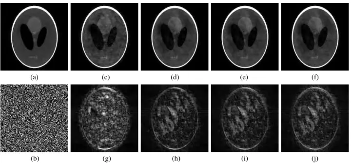
FIGURE 5. (a) Fully sampled image of simulated dataset; (b) random sampling mask; (c) reconstruction result of SAKE method; (d) reconstruction result of PCLR method with whole sampling data; (e) reconstruction result of PCLR method with 90% sampling data; (f) reconstruction result of PCLR method with 80% sampling data; (g)-(j) the reconstruction errors multiplied by 5 corresponding to reconstruction results (c)-(f) respectively.
which can be also written in the form of B(a) = (Bx(a), By(a), Bz(a)) The sensitivity Siis defined as Si(a) =
Bx(a)−jBy(a) [32]. Then, we can obtain Si(x, x) = Bx(x, x)−
jBy(x, x), with ϕSi(x, x) = arctan(−
By(x,x)
Bx(x,x)).ϕSi has smooth
phase since magnetic flux density varies slowly. We can see from the equation 22 the phase of the image of each channel is the linear addition of the phase of the sensitivity and the phase of the original object. Considering the phase of the sensitivity is varying slowly, it is determined by the original object whether the phase of channel image is smooth or not. In the PCLR method we are assuming that the channel images phase changing slowly which could explain that the PCLR method has better effect on the objects whose phase is smooth. And we can also see this in the comparison between the results of the simulation experiments and the real data experiments.
Therefore, the phase of each underlying magnetization image, ϕρi(x, y), varies slowly. Thus, a parallel imaging Shepp-Logan phantom k-space dataset with slowly varying phase in each underlying magnetization image was synthe-sized with the size of 180 × 180 × 8.
Fig.5shows the reconstruction result and error of simu-lation dataset under 30 percent sampling ratio, using 5 × 5 truncation neighborhood with Fig. 5(c) for SAKE method and Fig. 5(d)-(f) for PCLR method respectively.Compared with the fully sampled reconstruction image, the two small light phantoms in the medial axis and three tiny phantoms in the bottom are not well reconstructed in this sampling and reconstruction conditions. Fig.5(c) is reconstructed by SAKE with the 30 percent sampling dataset. Fig. 5(d)-(f) are reconstructed by PCLR method with 100 percent, 90 percent and 80 percent sample acquisition respectively after the same 30 percent sampling on the original dataset.
The aforementioned five phantoms are clearly reconstructed with all sample acquisition by using PCLR method. The two light phantoms in the medial axis get slowly blurred as the reduction of the usage of sample acquisition.
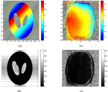
Fig.6 shows the phase of the simulated dataset and the phases of the coil images. Fig.6(a) is the phase of the original image, and Fig.6(b) shows its smoothness. Phase for each pixel the value ranges from −180 to 180, and we calculate the differences between one pixel and its neighborhoods, the right and bottom of it. For the absolute values of the differences larger than 180, we change it by minusing 360 (for two pixels, −179 and 179, the difference is 2). And the smoothness of the phase ranges from 0 to 360 in the Fig.6(b) and the smaller values represent the phase changing more slowly.
As shown in Fig.7, its the Error-Iterations curves. For each channel, the error is defined as the difference between the Frobenius norms of recovering k-space and the complete k-space then divided by the Frobenius norm of the complete k-space, as an example, the following equation shows the error of 2-D matrixes A and B:
Error = |FroNorm(B) − FroNorm (A)|
FroNorm(A) (24)
The FroNorm() calculate the Frobenius norm of the matrix which is also the sum of the root of the sigular values of the matrix. As the number of iterations increases, the rate of relative error reduction slows down, that is to say, the conver-gence rate slows down. And when the number of iterations reaches 100, the relative error has been lower than 2%, and the convergence rate becomes slow enough, close to 0, we think that the iteration can be stopped.
Three dimensional figures of SSIM with the change of sampling ratio and truncation neighborhood for simulation
FIGURE 6. (a) Phase of the simulated dataset; (b) smoothness of simulated dataset; (c)-(j) phases of the 8 coil images of the simulated dataset, respectively.
FIGURE 7. The ralative error between the recovering k-space data after each iteration and the complete k-space data (for the simulated data, and the neighborhoods size 5 × 5,λ = 0.1) with (a) for each channel and (b) the sum of the channels.
data and real data are shown in Fig. 8(a). The variation of SSIM with the change of sampling ratio and the change of truncation neighborhood is shown in Fig.8(b) and Fig.8(c). It can be seen from Fig.8(b) that SSIM value increases slowly for both SAKE and PCLR methods with neighborhood larger than 5 × 5. It is mainly because the Fourier truncation is almost precise, and the expansion of truncation neighborhood has insignificant enhancement of reconstruction result. Com-pared with Fig.5(c), both Fig.5(d)-(f) intuitively shows better reconstruction results and less reconstruction error, which also can be reflected in Fig.8(a).
The image reconstructed by PCLR has larger SSIM value than the corresponding one reconstructed by SAKE under each missing rate ranging from 50 percent to 80 percent, which means the PCLR method has better structural sim-ilarity to the original magnetization image. In particular, the PCLR with 80 percent data acquisition has slightly difference between the one with complete data acquisition
and still shows better reconstruction effect than SAKE. It reflects that PCLR could be competent for the par-tial Fourier transform when comparing the results and the assessment.
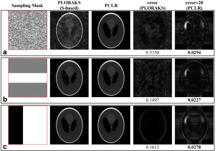
To further illustrate the performance of the pro-posed algorithm, its performance is compared to S-based P-LORAKS, which shows better performance than C-based P-LORAKS [22], in Fig 9. For both P-LORAKS and PCLR, the maximum iteration number and the truncation neighbor-hood were set 200 and 5*5. The second and third columns show reconstructed images using a linear grayscale (normal-ized to make image intensities in the range from 0 to 1), while the fourth and fifth columns show error images (The error of PCLR is magnified 20 times for a better visualization). NRMSE values are shown underneath each error image, with the best NRMSE values highlighted with bold text. Obvi-ously, PCLR results were better than S-based P-LORAKS reconstruction.
FIGURE 8. (a) Variation of SSIM value with different selection of truncation neighborhood and sampling ratio; (b) variation of SSIM value with different selection of truncation neighborhood under 30% sampling ratio; (c) variation of SSIM value with different selection of sampling ratio under 5 × 5 truncation neighborhood.
C. REAL DATASET
The real dataset, a brain image, was acquired with a T1-weighted, 3-D spoiled gradient echo sequence and it per-formed on a 1.5T MRI scanner (GE, Waukesha, Wisconsin, USA) using an eight-channel receive-only head coil. Its fully sampled reconstruction image is shown as Fig. 10(a). Scan parameters were set to echo time = 8 ms, pulse repetition time = 17.6 ms, and flip angle = 20◦. Imaging parameters were chosen such that FOV = 20cm × 20cm × 20cm with a matrix size of 200 × 200 × 200 for an isotropic resolution. A single axial slice was selected from this data set and was used throughout the experiments. Its fully sampled recon-struction result is shown as Fig. 10(a). Fig. 10 shows the reconstruction result and error multiplied by 5 of real dataset under 30 percent sampling ratio of random mode and 5 × 5 truncation neighborhood with Fig.10(c) for SAKE method and Fig. 10(d)-(f) for PCLR method respectively. And the
SAKE and PCLR reconstruction all did after the 30 percent sampling on the fully sampled dataset.
Fig.11shows the phases of the 8 coil images of the real dataset. We cant have the original image of the real dataset, so we cant provide the phase of the original image. But considering the phase changing slowly of the sensitivity of the coils, we can take one of the phases as an alternative. We take the sixth phase, Fig.11(f) to represent the phase of the image of the real dataset, and we show its smoothness together with the one of simulated dataset in Fig.15.
A little difference appears when the real data is taken into consideration. In Fig.10, PCLR method does not show the same superiority as it performs in the simulation experiment compared with SAKE. We can see both the phases of the simulated data and the real data in Fig. 15, together with corresponding smoothness. By this method, we can find the phase of simulated data is more smooth in the ROI which can
FIGURE 9. Reconstruction results for the Shepp-Logan phantom. a: Random sampling. b: Structured sampling. c: Random partial Fourier sampling. From left to right, the second and third columns show the results using P-LORAKS (S-based) and PCLR, respectively, while the fourth and fifth columns show error images. (The error of PCLR is magnified 20 times for a better visualization.) NRMSE values are shown underneath each error image, with the best NRMSE values highlighted with bold text.
explain the better performance for the simulated experiments. Fig. 15(d) shows a round white in the ROI which corre-sponding the larger error in Fig.10(h) the same round. The reconstruction results of the two methods are almost the same. Then, the situation of sampling under the radial sampling is tested and shown in Fig.12. Unlike random sampling mode, reconstruction results of PCLR method have significantly less error than that of SAKE method in the situation of radial sampling, especially the inner of brain, which is also the key area in diagnoses. Moreover, PCLR method has better performance than SAKE method especially under the low sampling rate because the constraint of linear correlation becomes weak and the phase constraint plays an important role.
Fig.13shows the denoising capability of the two meth-ods. Sampling ratio and truncation neighborhood are set to 40 percent and 5 × 5. It can be seen from figure that PLCR method has better denoising performance and the superiority enlarges especially when the SNR is decreasing. Fig. 14
shows the reconstruction results and errors under the 30db SNR (The noise is directly added to the k-space data).
Tab. 1 display the reconstruction time of the both two methods with 5 × 5 truncation neighborhood. The recon-struction time of each method has a proportional relationship with quantity of data acquisition used in the reconstruction process. According to Tab. 1 , PCLR method reconstructed with the whole data acquisition has slightly longer time than SAKE. The reconstruction time of the one with incomplete data acquisition depends on the usage ratio of data acquisi-tion. For instance, 80 percent data acquisition was used in PCLR method and then 20 percent reconstruction time was saved compared to the SAKE method.
At first glance, it seems the reconstruction time should increase as the sampling rate decreases. Actually in the pro-posed technique PCLR, by the unique way of the construction of the data matrix, the size of the data matrix decreases as the sampling rate decreases. In addition, the rank of the data matrix is related to the number of sampling in the truncation neighborhood [17]. Lower truncation means lower rank of the data matrix. With the smaller size and lower rank, the SVD of the data matrix, which is accounting for the main time assumption, takes less time in one iteration. So the
FIGURE 10. (a) Fully sampled image of real dataset; (b) random sampling mask; (c) reconstruction result of SAKE method; (d) reconstruction result of PCLR method with whole sampling data; (e) reconstruction result of PCLR method with 90% sampling data; (f) reconstruction result of PCLR method with 80% sampling data; (g)-(j) the reconstruction errors multiplied by 5 corresponding to reconstruction results (c)-(f) respectively.
FIGURE 11. (a)-(h) Phases of the 8 coil images of the real dataset, respectively.
TABLE 1. The reconstruction time with both SAKE and PCLR for real dataset.
reconstruction time decreases as showed in the Tab. 1 which recorded all for 100 iterations.
V. DISCUSSION
The proposed algorithm has essential differences with the P-LORAKS [22], and the E-SPIRiT [33] which have
been published recently. The proposed method’s novelty lies in automatically considering two constraints simulta-neously.The processing automatically provides a tradeoff between the two constraints for an optimized reconstruction. It guarantees that a best reconstruction is obtained auto-matically, which is essential from a practical perspective.
FIGURE 12. (a) Fully sampled image of real dataset; (b) radial sampling mask; (c) reconstruction result of SAKE method; (d) reconstruction result of PCLR method with whole sampling data; (e) reconstruction result of PCLR method with 90% sampling data; (f) reconstruction result of PCLR method with 80% sampling data; (g)-(j) the reconstruction errors multiplied by 5 corresponding to reconstruction results (c)-(f) respectively.
FIGURE 13. Variation of SSIM value with different selection of SNR.
Specifically, first, both P-LORAKS and PCLR are the models on parallel MRI reconstruction with phase constraint. Dif-ferences exist in implementing the two models. Both linear relationship and phase constraint are concerned in the two models. In P-LORAKS model, the two constraints are utilized as two separated regularization term in solving the optimiza-tion of parallel k-space dataset. There are two parameters and in P-LORAKS reconstruction formula (Eq.12). In the experiments, P-LORAKS model can only a single constraint, either linear relationship or phase constraint, corresponding to C-based P-LORAKS and S-based P-LORAKS. Moreover, when the two submodels achieve their own optimization, their combination is not the optimal solution, which appar-ently shows the two constraint are implemented respectively.
In PCLR model, both linear relationship and phase constraint are combined together to construct a revised data matrix whose entries come from the original k-space dataset. Only one parameter that balances the linear relationship and phase constraint is utilized in reconstruction process. It means that the single parameter can decide the optimal solution of recon-struction. The comparison of experiment results confirms this theoretical analysis. As for E-SPIRiT model, it is an impor-tant reconstruction method based on the SENSE framework. It applies block strategy to sensitivity map. E-SPIRiT model still needs sensitivity map, which consumes longer time and is abandoned in P-LORAKS and PCLR.
The SAKE reconstruction which only takes linear corre-lation of k-space data into consideration cannot hold good performance with the increasing missing rate. However, the proposed PCLR with extra phase constraint performs better. The reconstruction results of simulation dataset demonstrate the superiority of PCLR in reconstructing multi-channel k-space dataset with smooth phase in underlying magneti-zation image. In addition, for the real dataset of brain, the reconstruction result of PCLR with complete data acqui-sition is still better than that of the SAKE method under each missing rate. Moreover, when the missing rate exceeds 70 percent, the PCLR with incomplete data acquisition has better reconstruction capacity as well, which means PCLR could save k-space samples to achieve the same or even slightly better reconstruction performance compared with SAKE.
PCLR shows superiority with high missing rate mainly results from introduction of phase constraint. The regular lin-ear correlation constraint performs well with high sampling rate as the prediction could be accurate with more known
FIGURE 14. (a) Fully sampled image of real dataset; (b) random sampling mask; (c) reconstruction result of SAKE method; (d) reconstruction result of PCLR method with whole sampling data; (e) reconstruction result of PCLR method with 90% sampling data; (f) reconstruction result of PCLR method with 80% sampling data; (g)-(j) the reconstruction errors multiplied by 5 corresponding to reconstruction results (c)-(f) respectively.
FIGURE 15. (a) Phase of the original image of the simulated dataset; (b) smoothness of (a); (c) phase of the 6-th coil image of the real dataset; (d) smoothness of (c).
k-space data based on the linear correlation. As the sampling rate declines, the linear correlation constraint becomes invalid gradually. However, the phase information describes the rel-ative position relationship of the data, even with high missing rate, it still utilizes the relationship to estimate the missing data effectively.
It concludes that the local unsmooth phase in magnetiza-tion image would affect the PCLR reconstrucmagnetiza-tion result based the comparison between the simulated Shepp-Logan phan-tom dataset and real brain dataset. The local inconsistency of
phase restricts the effect of phase constraint. The decline of phase constraint factor,λ can achieve better reconstruction results for PCLR methods. And the further research could focus on exploring the ranges of the parameterλ for better performances for different objects.
As for another parameter, the truncation neighborhood size, which is responsible for both the performance and the time cost of the reconstruction. The performance will get better as the truncation neighborhood size increases which means it can provide more information for reconstruction. But at the same time, the time cost of the reconstruction will increase. Actually, when the size reaches 11 × 11, the information the neighborhoods provide is enough.
Reconstruction time depends on the size of constructed data matrix. The constructed data matrix of PCLR with com-plete data acquisition is almost the same as but slightly larger than that of SAKE. The reconstruction time of the two meth-ods takes almost the same. Nevertheless, both reconstruction time and data acquisition save approximately corresponding proportion with the application of PCLR with incomplete data acquisition.
VI. CONCLUSION
In this paper, we propose a multiple-channel MRI recon-struction method based on Low-rank matrix completion with phase constraints, which uses both linear dependent relationship and phase constraint in a single reconstruction procedure. In contrast to SAKE model, it just takes phase constraint into consideration and unlike the newly proposed P-LORAKS model it utilizes the two constraints in a single step, which means that only one parameter can make sure the novel algorithm get the optimal solution of reconstruction.
Results of the simulations and experiments illustrate that our proposed algorithm has a series of superiorities, such as the reduction of k-space acquisition and reconstruction time, to these comparative algorithms.
REFERENCES
[1] J. Carlson and T. Minemura, ‘‘Imaging time reduction through multiple receiver coil data acquisition and image reconstruction,’’ Magn. Reson. Med., vol. 29, no. 5, pp. 681–687, 1993.
[2] Y. Zhang et al., ‘‘Image processing methods to elucidate spatial character-istics of retinal microglia after optic nerve transection,’’ Sci. Rep., vol. 6, Feb. 2016, Art. no. 21816.
[3] Y. Zhang, S. Wang, G. Ji, and Z. Dong, ‘‘Exponential wavelet iterative shrinkage thresholding algorithm with random shift for compressed sens-ing magnetic resonance imagsens-ing,’’ IEEJ Trans. Electr. Electron. Eng., vol. 10, no. 1, pp. 116–117, 2015.
[4] Y. D. Zhang, S. Wang, P. Phillips, Z. Dong, G. Ji, and J. Yang, ‘‘Detection of Alzheimer’s disease and mild cognitive impairment based on structural volumetric MR images using 3D-DWT and WTA-KSVM trained by PSOTVAC,’’ Biomed. Signal Process. Control, vol. 21, pp. 58–73, Aug. 2015.
[5] Y. Zhang and L. Wu, ‘‘Improved image filter based on SPCNN,’’ Sci. China Ser. F, Inf. Sci., vol. 51, no. 12, pp. 2115–2125, 2008.
[6] Y. Zhang, L. Wu, S. Wang, and G. Wei, ‘‘Color image enhancement based on HVS and PCNN,’’ Sci. China Inf. Sci., vol. 53, no. 10, pp. 1963–1976, 2010.
[7] Z.-P. Liang, F. Boada, R. T. Constable, E. M. Haacke, P. C. Lauterbur, and M. R. Smith, ‘‘Constrained reconstruction methods in MR imaging,’’ Rev. Magn. Reson. Med., vol. 4, no. 2, pp. 67–185, 1992.
[8] J. P. Haldar, ‘‘Low-rank modeling of local k-space neighborhoods (LORAKS) for constrained MRI,’’ IEEE Trans. Med. Imag., vol. 33, no. 3, pp. 668–681, Mar. 2014.
[9] F. Huang, W. Lin, and Y. Li, ‘‘Partial fourier reconstruction through data fitting and convolution in k-space,’’ Magn. Reson. Med., vol. 62, no. 5, pp. 1261–1269, 2009.
[10] D. K. Sodickson and W. J. Manning, ‘‘Simultaneous acquisition of spa-tial harmonics (SMASH): Fast imaging with radiofrequency coil arrays,’’ Magn. Reson. Med., vol. 38, no. 4, pp. 591–603, 1997.
[11] K. P. Pruessmann, M. Weiger, M. B. Scheidegger, and P. Boesiger, ‘‘SENSE: Sensitivity encoding for fast MRI,’’ Magn. Reson. Med., vol. 42, no. 5, pp. 952–962, 1999.
[12] M. A. Griswold et al., ‘‘Generalized autocalibrating partially par-allel acquisitions (GRAPPA),’’ Magn. Reson. Med., vol. 47, no. 6, pp. 1202–1210, 2002.
[13] M. Lustig and J. M. Pauly, ‘‘SPIRiT: Iterative self-consistent parallel imag-ing reconstruction from arbitrary k-space,’’ Magn. Reson. Med., vol. 64, no. 2, pp. 457–471, 2010.
[14] J. Zhang, C. Liu, and M. E. Moseley, ‘‘Parallel reconstruction using null operations,’’ Magn. Reson. Med., vol. 66, no. 5, pp. 1241–1253, 2011. [15] K. H. Jin, D. Lee, and J. C. Ye, ‘‘A novel k-space annihilating filter method
for unification between compressed sensing and parallel MRI,’’ in Proc. IEEE 12th Int. Symp. Biomed. Imag. (ISBI), Apr. 2015, pp. 327–330. [16] G. Ongie and M. Jacob, ‘‘Super-resolution MRI using finite rate of
inno-vation curves,’’ in Proc. IEEE 12th Int. Symp. Biomed. Imag. (ISBI), Apr. 2015, pp. 1248–1251.
[17] P. J. Shin et al., ‘‘Calibrationless parallel imaging reconstruction based on structured low-rank matrix completion,’’ Magn. Reson. Med., vol. 72, no. 4, pp. 959–970, 2014.
[18] A. A. Samsonov, E. G. Kholmovski, D. L. Parker, and C. R. Johnson, ‘‘POCSENSE: POCS-based reconstruction for sensitivity encoded magnetic resonance imaging,’’ Magn. Reson. Med., vol. 52, no. 6, pp. 1397–1406, 2004.
[19] C. Lew, D. Spielman, and R. Bammer, ‘‘TurboSENSE: Phase estimation in temporal phase-constrained parallel imaging,’’ in Proc. 11th Sci. Meeting (ISMRM), Kyoto, Japan, 2004, p. 2646.
[20] J. D. Willig-Onwuachi, E. N. Yeh, A. K. Grant, M. A. Ohliger, C. A. McKenzie, and D. K. Sodickson, ‘‘Phase-constrained parallel MR image reconstruction,’’ J. Magn. Reson., vol. 176, no. 2, pp. 187–198, 2005. [21] M. Bydder and M. D. Robson, ‘‘Partial Fourier partially parallel imaging,’’
Magn. Reson. Med., vol. 53, no. 6, pp. 1393–1401, 2005.
[22] J. P. Haldar and J. Zhuo, ‘‘P-LORAKS: Low-rank modeling of local break k-space neighborhoods with parallel imaging data,’’ Magn. Reson. Med., vol. 75, no. 4, pp. 1499–1514, 2016.
[23] M. Uecker et al., ‘‘ESPIRiT—An eigenvalue approach to autocalibrat-ing parallel MRI: Where SENSE meets GRAPPA,’’ Magn. Reson. Med., vol. 71, no. 3, pp. 990–1001, 2014.
[24] G. Heinig and P. Jankowski, ‘‘Kernel structure of block Hankel and Toeplitz matrices and partial realization,’’ Linear Algebra Appl., vol. 175, pp. 1–30, Oct. 1992.
[25] J.-F. Cai, E. J. Candes, and Z. Shen, ‘‘A singular value threshold-ing algorithm for matrix completion,’’ SIAM J. Optim., vol. 20, no. 4, pp. 1956–1982, 2010.
[26] E. J. Candès and B. Recht, ‘‘Exact matrix completion via convex optimiza-tion,’’ Found. Comput. Math., vol. 9, no. 6, pp. 717–772, 2009. [27] J. A. Cadzow, ‘‘Signal enhancement—A composite property mapping
algorithm,’’ IEEE Trans. Acoust., Speech Signal Process., vol. 36, no. 1, pp. 49–62, Jan. 1988.
[28] Z. Wang, A. C. Bovik, H. R. Sheikh, and E. P. Simoncelli, ‘‘Image quality assessment: From error visibility to structural similarity,’’ IEEE Trans. Image Process., vol. 13, no. 4, pp. 600–612, Apr. 2004.
[29] A. M. Eskicioglu and P. S. Fisher, ‘‘Image quality measures and their performance,’’ IEEE Trans. Commun., vol. 43, no. 12, pp. 2959–2965, Dec. 1995.
[30] Z. Wang and A. C. Bovik, ‘‘A universal image quality index,’’ IEEE Signal Process. Lett., vol. 9, no. 3, pp. 81–84, Mar. 2002.
[31] L. A. Shepp and B. F. Logan, ‘‘The Fourier reconstruction of a head section,’’ IEEE Trans. Nucl. Sci., vol. 21, no. 3, pp. 21–43, Jun. 1974.
[32] M. Guerquin-Kern, L. Lejeune, K. P. Pruessmann, and M. Unser, ‘‘Realistic analytical phantoms for parallel magnetic resonance imaging,’’ IEEE Trans. Med. Imag., vol. 31, no. 3, pp. 626–636, Mar. 2012. [33] M. Uecker and M. Lustig, ‘‘Estimating absolute-phase maps using
espirit and virtual conjugate coils,’’ Magn. Reson. Med., vol. 77, no. 3, pp. 1201–1207, 2017.
LONGYU JIANG (M’13) received the Ph.D. degree in signal processing from Grenoble Univer-sity, Grenoble, France, in 2013. Since 2013, she has been a Faculty Member with the Department of Computer Science and Engineering, Southeast University, Nanjing, China. Her major research interests include MRI image reconstruction and array signal processing.
RUNGUO HE received the M.S. degree in com-puter science and engineering from Southeast University, Nanjing, China, in 2015. His major research interest is MRI image reconstruction.
JIE LIU is currently pursuing the Ph.D. degree in computer science and engineering with Southeast University, Nanjing, China. His major research interest is MRI image reconstruction.
YANG CHEN (M’12) received the M.S. and Ph.D. degrees in biomedical engineering from First Mil-itary Medical University, Guangzhou, China, in 2004 and 2007, respectively. Since 2008, he has been a Faculty Member with the Department of Computer Science and Engineering, Southeast University, Nanjing, China. His research inter-ests include medical image reconstruction, image analysis, pattern recognition, and computerized-aid diagnosis.
JIASONG WU (M’09) received the B.S. degree in biomedical engineering from the University of South China, Hengyang, China, in 2005, and the joint Ph.D. degree with the Laboratory of Image Science and Technology (LIST), Southeast University, Nanjing, China, and the Laboratoire Traitement du signal et de l’Image, University of Rennes 1, Rennes, France in 2012. He is currently with LIST as a Lecturer. His research interests mainly include fast algorithms of digital signal processing and their applications. He received the Eiffel Doctorate Schol-arship of Excellence (2009) from the French Ministry of Foreign Affairs and the Chinese Government Award for outstanding self-financed student abroad (2010) from the China Scholarship Council.
HUAZHONG SHU (SM’06) received the B.S. degree in applied mathematics from Wuhan Uni-versity, Wuhan, China, in 1987, and the Ph.D. degree in numerical analysis from the Univer-sity of Rennes, Rennes, France, in 1992. He is currently a Professor with the Department of Com-puter Science and Engineering, Southeast Uni-versity, Nanjing, China. His research interest is involved in the image analysis, pattern recognition, and fast algorithms of digital signal processing.
JEAN-LOUIS COATRIEUX (LF’16) received the Ph.D. and State Doctorate degrees in sciences from the University of Rennes 1, Rennes, France, in 1973 and 1983, respectively. His experience is related to 3-D images, signal processing, com-putational modeling, and complex systems with applications in integrative biomedicine. He has authored more than 300 papers in journals and conferences and edited many books in his research areas.