Astrophysical applications of the Einstein ring gravitational lens, MG1131+0456

ASTROPHYSICAL APPLICATIONS OF THE EINSTEIN RING

GRAVITATIONAL LENS, MG1131+0456

by

GRACE HSIU-LING CHEN

Bachelor of Science, San Francisco State University, 1990

SUBMITTED TO THE DEPARTMENT OF PHYSICS IN PARTIAL FULFILLMENT OF THE REQUIREMENTS

FOR THE DEGREE OF

DOCTOR OF PHILOSOPHY

at the

MASSACHUSETTS INSTITUTE OF TECHNOLOGY

May 1995

Copyright Q1995 Massachusetts Institute of Technology All rights reserved

Signature of Author: Certified by: Accepted by: Department of Physics May 1995 Jacqueline N. Hewitt Thesis Supervisor George F. Koster

Chairman, Graduate Committee

JUN 2 6 1995

ASTROPHYSICAL APPLICATIONS OF THE EINSTEIN RING GRAVITATIONAL LENS, MG1131+0456

by

GRACE HSIU-LING CHEN

ABSTRACT

MG1131+0456 has been observed extensively with the Very Large Array tele-scope, and its complex morphology has provided the opportunity for investigating three important astrophysical problems: (1) the mass distribution in the lens galaxy, (2) the structure of the rotation measure distribution in the lens, and (3) the possi-bility of using the system to constrain the Hubble parameter.

We determine the mass distribution of the lens galaxy by modeling the multifre-quency VLA images of the system. Among the models we have explored, the profile of the surface mass density of the best lens model contains a substantial core radius and declines asymptotically as r- 1_2±0'_{2. The mass inside the lens enclosed by the}

average ring is very well constrained. If the source is at redshift of 2.0 and the lens is at redshift of 0.5, the mass of the lens enclosed by the ring radius is - 2.0 x 1011 solar mass.

We develop a new technique to determine the structure of the rotation measure

distribution in the lens. We have detected variations in the rotation measure

distri-bution in the lens galaxy of MG1131, and the structure of the variations indicates that the magnetic field in the lens galaxy is likely to change on a scale of 1".

The VLA observations of MG1131+0456 at 8 and 15 GHz taken at several epochs show that the compact components in the system are weakly variable. Results of Monte Carlo simulations show that a time delay should be measurable if ap-proximately 100 observations are obtained. Hence, one should seriously consider MG1131+0456 for measuring the Hubble parameter.

Table of Contents

1 Introduction ... 2

1.1 History of Gravitational Lenses ... 2

1.2 Theory of Gravitational Lensing .... ... 3

1.2.1 Gravitational Lensing Optics ... 4

1.2.2

Image

Multiplicities

. .. . . ... 8

1.2.3 Simple Lens Models ... 9

1.3 Applications of Gravitational Lensing ... 10

1.3.1 Mass Distribution of the Lens . ... .. ... 10

1.3.2 Cosmography ... 12

1.4 Einstein Ring Lens System, MG1131+0456 ... 14

1.5 Outline ... 16

2 High Angular Resolution Radio Observations . ... 20

2.1 Two Element Interferometry ... 20

2.2 Observations ... 23

2.3 Calibration and Mapping ... 26

3 Radio Morphology and Nature of MG1131+0456 . ... 32

3.1 Maps of Total Intensity and Polarized Emission ... . 32

3.2 What is Component D? ... 37

3.2.1 Is D the Lensed image of C? . ... 37

3.2.2 Is D the Radio Image of the Lens Galaxy? ... 41

3.2.3 Is D the Odd Image of the System? ... 45

3.3 Spectral Index Measurements of All Components ... 45

3.4 Depolarization Structure ... ... 48

4 Methodology of the Lens Modeling ... 55

4.2 Potentials Used for the Modeling ... 4.2.1 de Vaucouleurs Model ...

4.2.2 a Model ...

4.2.3 Qualitative Analysis of the a model ... 4.3 A Summary of the LensClean Algorithm ...

4.3.1 CLEAN ...

4.3.2 LensClean.

...

...

4.4 Optimizing the Lens Parameters in Multi-Dimensional 4.5 Error Estimation and Goodness of Fit ...

5 Results of the Lens Modeling ....

5.1 8 GHIz Result ...

5.1.1 de Vaucouleurs Models... 5.1.2 a, Models ...

5.1.3 Can the Nature of D Bias

5.2 5 and 15 GHz Model ...

5.3 Two Nearby Galaxies ... 5.4 Conclusion ... ... ... .

....

the . . .. .. o... ... .. ... ... .... ... ... ...

Result?

...

. . . .. . .. ... ... .. . . .. . . . .. . . .. . . .. .... ...,,...

6. Probing the Structure of the Rotation Measure in Highly-Redshifted Galaxies with Gravitational Lenses ...

6.1 6.2 6.3 6.4 6.5 6.6 6.7

Determination of the Rotation Measure in MG1131+0456 Physical Considerations and the ARM Measurements... Effects due to the Galaxy ...

Effects due to the Plasma Around the Source ...

Effects due to the Intergalactic Medium ...

Discussion

...

Conclusion

...

113 .... 113 ... 124 ... 126 ... 127

...

134

...

135

...

137

58 60 61 63 65 65 68 69 70 . . . . .. ... . .. . . . .. . . . . .. . . .. . . . .. . . .. . .. ... ... .o . v. v. . o Space ... .. . . . 77 77 77 83 95 97 101 109

7. The Possibility of Measuring the Hubble Parameter

from MG1131+0456 . ... 140

7.1 Variability of the Compact Components ... 140

7.1.1 8 GHz

...

141

7.1.1.1L Data Analysis ... 141

7.1.1.2 Error Estimates ... ... 144

7.1.1.3 Evidence for variability ... 146

7.1.2 15 GHz ... 149

7.2 Is the Time Delay in MG1131+0456 Measurable? ... 154

7.3 Conclusion: The Prospect of Measuring the Hubble Parameter 158 8 Summary ... 161

Acknowledgement

I could not have completed this thesis without the following people's support and

love ....

First of all, I would like to thank my thesis advisor, Prof. Jacqueline N. Hewitt, for giving me the opportunity to conduct researches in the field of gravitational lensing and the support and encouragement she has been given me in the last five years. I would also like to thank Prof. Christopher S. Kochanek, from whom I have learned how to attack problems critically, and Dr. Edward Fomolont, who was always there for giving me valuable advice on analyzing the VLA data.

There are no words big enough to express my gratitude for the the love my parents, sister, and brother have given me. Without their support and their beliefs on my ability, I would have left MIT four years ago, and this thesis would have never been written.

I would also like to thank Charlie K., Sam, Debbie, Chris, Max, Andre, Lori, Cathy, John E., John C., Frowny, Ann C., Ann S., and Prof. Bernard Burke for making the MIT radio group a pleasant place to work in. I would like to thank Debbie, Charlie, and Cathy, especially, for taking the time to proofread this thesis

carefully.

To Charlie Collins, I would have gone insane by now without the laughters your son, Michael, and your wife have brought during our routine lunches on Monday.

Thank you all!

Finally, I would like to thank a very special friend, my Bdr, for his unmeasurable love and care. I will always treasure the time we have spent together here.

1. Introduction

1.1 History of Gravitational Lenses

The idea that a light ray can be deflected by the presence of a massive object was first considered by Sir Isaac Newton in the early 1700s. One hundred years later, based on Newtonian gravitational theory, Soldner calculated the deflection of the light ray from its straight path when it passes by a massive object (Soldner 1804). After another one hundred years, Einstein performed the same calculation using his theory of general relativity and obtained a result that is twice as the value predicted by Soldner (Einstein 1915). In 1919, Dyson set up an experiment to measure the deflection of a starlight passing by the limb of the sun during a solar eclipse and confirmed Einstein's prediction (Dyson 1919). Later in that year, Lodge (1919) introduced the interesting idea that it is possible for a gravitational potential to be strong enough to create more than one image of a background source. Chwolson (1924) and Einstein (1936) both applied Lodge's idea of multiple imaging to nearby stars and concluded that the angular separation between the images would be too small to be resolved by ground-based optical telescopes and that the phenomenon of multiple imaging would not be observable. It did not take the ingenious Zwicky long to realize that not only stars but also distant galaxies could act as lenses (Zwicky 1937). in that case, the angular separation between a pair of images would be detectable, and furthermore, if detected, the gravitational lens system could be used for numerous astrophysical applications. In Zwicky's 1937 paper, he stated:

The discovery of images of nebulae which are formed through the gravita-tional fields of nearby nebulae would be of considerable interest for a number of reasons.

(1) It should furnish an additional test for the general theory of relativity. (2) It would enable us to see nebulae at distances greater than those ordi-narily reached by even the greatest telescopes....

(3) ...Observations of the deflection of light around nebulae may provide the most direct determination of nebular masses ....

2;wicky's pioneering ideas led the field of gravitational lensing to extragalactic

astron-omy.

After 1937, the field remained dormant for roughly thirty years. New applications, such as the use of gravitational lenses for distance measurements (Klimov 1963; Liebes 1964; Refsdal 1964, 1966) and as probes to determine the stellar composition (Chang & Refsdal 1979) were considered in 1960's and 1970's. However, the field remained as an esoteric playground for relatively few theorists during that period. The situation changed in 1979 after the discovery of the first gravitational lens system (Walsh, Carswell, & Weymann 1979). As part of a project identifying the optical counterparts to sources in a radio survey at 996 MHz (Cohen et al. 1977), Walsh et al. (1979) discovered a system, named Q0957+561, consisting of two compact components both at redshifts of z2 - 1.4. The similarities between their spectra and the presence of a lensing galaxy at z 0.36 (Stockton 1980; Young et al. 1980) verified the lensing hypothesis. After the discovery, many began to show tremendous interest in the field

of lensing, and numerous papers concerning both observational and theoretical work appeared. The second gravitational lens system was discovered only one year later (Weymann et al. 1980). In 1986, a second type of lens, a long circular arc with angular radius 25" in Abell 370, was discovered by Soucail et al. (1987), and in L1987, a third type of lens, a ring (known as MG1131+0456), was discovered by Hewitt et al. (1988) as part of the radio lens survey project conducted at MIT (Hewitt 1986;

Lehr 1991).

At the present time, there are more than 20 confirmed lenses, and more are waiting to be discovered. The field of gravitational lensing is no longer considered an "esoteric field" but one of the most active fields in extragalactic astronomy.

1.2 Theory of Gravitational Lensing

of this thesis, presenting a complete discussion of the theory of gravitational lensing would not be appropriate. Instead, only the basic notions, concepts, and theories of gravitational lensing relating to this thesis will be discussed. A complete treatment of gravitational lensing theory is presented in the book, Gravitational Lenses (Schneider, Ehlers, & Falco 1992). Several excellent review papers on the subject (Blandford & Kochanek 1987; Canizares 1987; Blandford & Narayan 1992) are also available in the literature. These sources are recommended for readers seeking a more thorough discussion of this subject.

1.2.1 Gravitational Lensing Optics

In the most simple configuration, there are only a few elements in gravitational lensing optics: a source, S, a massive object acting as a lens, L, and an observer, 10. Figure 1.1 displays a schematic of the optics. The gravitational potential of the massive object (L) causes the light ray emitted from the source to be deflected from its straight path by an amount a', so the observer sees an image formed at an angular location x instead of u. If the gravitational potential of the lens is known, the amount of the bending, a (a = x - u) or a' = (D,,/Dol)a can be calculated exactly from Einstein's theory of general relativity. In an astrophysical setting, stars, globular clusters, galaxies, and galaxy clusters are all capable of producing lensing effects.

An elegant way to understand image formation in gravitational lensing is to utilize Fermat's principle. This idea was fully developed by Schneider (1985) and Blandford & Narayan (1986). Let us refer back to the optical geometry laid out in Figure 1.1. When the lens is absent, the light travels on the path SO; and when the lens is present, it travels on the path SPO. The light path in each case is the null geodesic of the met-ric connecting the observer and the source, and the light travel time can be calculated using the theory of general relativity. In a weak field approximation, the difference

I

%

P

S

L

|--

Dlis

I

o

0

Figure 1.1 - Basic geometry of gravitational lensing optics. A light ray from a source S at redshift z, is deflected due to the presence of the lens L. Assuming that the lens is thin compared to the total path length, the amount of deflection can be described by a single parameter a'. Because of the deflection, an observer sees the image of the source appearing at an angular position x instead of the true source position u. Dij are the angular diameter distances between the source, lens, and observer.

in the light travel time between these two paths, known as the time delay, has the form,

t(+z)[ DsD°(xu)2

t=( + )LD (x -u)

2

_{- 2}

_{ight path}c ds]c3 I ' (1 - 1)

Dij are the angular diameter distances between objects i and j, c is the speed of light, z denotes the redshift of the lens, and is the three-dimensional Newtonian potential of the lens. In general, Dij depends on the model of cosmology.

]Friedman cosmology, 2c ' Q,,H

(GiGj +

- 1)(Gj

-Gi) (1 + i)(1 + zji)2 In a

t----11%. I.. ; J

Gi = (1 + Qozi),

where Qo is the the density parameter, zi is the redshift of the object i, and H is the Hubble constant*. Each term in Eqn (1-1) represents a different physical process. The first term accounts for the extra path on which light needs to travel due to the presence of the lens, and the second term accounts for the delay in time when an object passes through a gravitational potential well as predicted by general relativity.

The three-dimensional Newtonian potential, , satisfies the Poisson equation,

V2, = 4rp, (1 - 3)

where p is the mass density of the lens. It is useful to define a rescaled two-dimensional Newtonian potential

DI,,

-d

4)ds

DosDol ght path C(12 _-4)

which also has a similar Poisson equation as Eqn (1-3),

V2¢ = 87rDOsDO E 2E (1-5)

Dl Ec

where E is the surface mass density and Ec = Dls/47rDosDol - the critical surface density - is the minimum surface density a homogeneous lens must have in order to produce multiple images (see discussion in Section 1.2.2). Expressing the time delay in terms of , we find

t = (1 + zl)DosDol [ (x-u)2_] (1 - 6)

Now we are ready to apply Fermat's principle. Fermat's principle states that light travels on a path that is stationary on the time surface, which means that images are formed on the extrema of the time surface. Applying this idea to Eqn (1-6), the location of the image x corresponding to the source u can be found at

u = - V(x),

(1 - 7)

* The Hubble constant is assumed to be Ho = 100h km Mpc- 1 _s- 1.

and the deflection angle a is

= VO. (1 - 8)

The gravitational deflection does not add emissivity to the light bundle or ab-sorb light from it, so the surface brightness of a bundle of light stays unchanged through gravitational lensing. However, the cross section of the bundle is altered by the deflection. Because of the change in the cross section, the image can appear larger (magnified) or smaller (demagnified) than the source size. The Jacobian of the transformation between u and x computes the ratio of the elemental areas in the two planes, so the image magnification can be evaluated effectively from the Jacobian. The magnification tensor, Mij, can be calculated as

Mij-

= U = [(s

-

aij)()]

1

,

(1

-

9)

and the total magnification is

M = det IMijl.

For a system containing a single deflector, the magnification tensor is symmetric, so the matrix can be diagonalized into

here p and p are diagonalized both real. The matrix provides an explicit

where pi and P2 are both real. The diagonalized matrix provides an explicit descrip-tion of the shape and size of the image. The shape of the image can be constructed by compressing or expanding the shape of the source by an amount 1/pi and 1/p2 along the principal axes. Because the eigenvalues are real, no rotation is involved. In general, the diagonalized matrix can be written in the form of

Mij=

1

·

0 K--Y

The quantity = 1 - E/EC governs the expansion or contraction along the principal axes and is known as the convergence. The quantity y governs the amount of shear

1.2.2 Image Multiplicities

From the structure of the lens equation (Eqn 1-7), it is clear that there is only one source corresponding to each image, but the converse is not true. In other words, depending on the potential of the lens, the mapping between u and x can be one-to-many, so a source can be lensed into more than one image.

The counting of images is rather simple; it is just the number of solutions which satisfy the relation

a

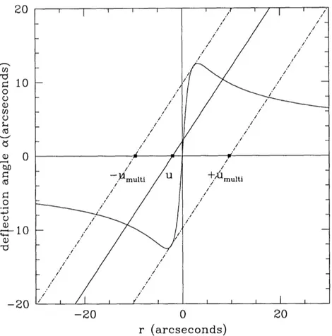
= V+(x) = x - u.

'One interesting characteristic of gravitational lensing is that the image multiplic-ity changes as a function of the source location. This concept can be most easily understood with graphical methods. For simplicity, we assume that has circular symmetry and that V0 is as shown by the curve in Figure 1.2. (The purpose of assuming circular symmetry is to reduce the lens equation to one dimension, so x-u is a straight line with its intercept on the abscissa representing the value of u. The result can be generalized to all other cases.) Depending on the source location, there can be one or more solutions. For the case demonstrated here (see Figure 1.2), there is (are) one (three) solution(s) if the location of source is at lul > Umlt (lul < Umult). The regions in which a source can be multiply imaged (i.e. lul < Umlt) are called the multiply imaged regions, and regions in which a source can only be singly imaged (i.e. ul > rmult) are called the singly imaged regions. When the source is crossing from a multiply imaged region to a singly imaged region, two images merge, magnify infinitely, and then disappear. The locus of the merging in the image plane is known as the critical line, and the associated locus in the source plane is called the caustic

line. In general, caustic lines divide the source plane into regions of image

multiplic-ity differing by -2. Of course, not all potentials are not strong enough to produce multiple images. The term weak lensing refers to the cases where the potentials are

incapable of multiple imaging whereas strong lensing refers to the other cases. 2:0 10 0 r) U) 0o C) ._ (0 _or, c) a, 10 on -20 0 20

r (arcseconds)

Figure 1.2 - A plot demonstrating the concept of multiple imaging in grav-itational lensing. For a given source at position u, the number of image corre-sponding to this source is just the number of solutions satisfying the lens equation a = Vq(x) = x - u. The solid curve represents V+(x). The solid straight line rep-resents the function x - u whose intercept on the abscissa denotes the value of u. When the source is located in the multiply imaged region (ul(umulIt), there are three solutions to the lens equation, hence three images. On the other hand, when the source is located in the region (lul) u,m,t), there is only one solution, hence one im-age. The boundary of the multiply imaged region is marked by the two dash-dotted lines.

1.2.3 Simple Lens Models

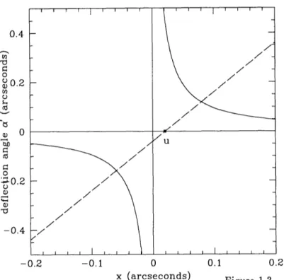
The simplest type of gravitational potential is that of a point mass. Light traveling past a point mass M is deflected by an amount a' = 4GM/c2 Dolx (where c = [L),IDos,,]a), where x is the image position (in arc seconds) relative to the point

mass. Figure 1.3 shows the deflection angle as a function of x produced by a point

I-mass with M = 10M® located at a distance 10 pc from the observer. The straight line in the figures represents the function a = x - u when the source is at 20 pc away from the observer. It is clear from Figure 1.3 that the multiply imaged region for a point mass lens extends to infinity, and sources at all positions, except at the optical axis,

will always be lensed into two images. When the source is on the optical axis, instead of two images, a ring of images with an angular radius of OE = V/4GMDis/c2 DDDo 1l

appears. The ring and E are generally referred to as the Einstein ring and the Einstein radius. For a source located at any other position u, two images appear at

+

= (u - u2 + 42 )/2. The flux magnifications associated with x± are M =

[2 i

/

(u

2

₊

_OE)+

_(u

2

_{+ OE)/u]/4.}

One other frequently used simple lens model is the singular isothermal sphere model. The surface mass density distribution in a singular isothermal sphere lens -has the form = 2_{/2GDox, where ro is the velocity dispersion of the objects in}

the lens galaxy. The simplicity of the potential and its ability to explain the flat rotation curve of spiral galaxies make it one of the "beloved" models for describing the potentials of galaxies or clusters of galaxies. The two-dimensional potential of this model is = br, where b = 47rDsr2_/D

o 2 sc (in arc seconds). The most peculiar

characteristic of this potential is the constant deflection angle (see Figure 1.4). As in the case of the point mass potential, a source on the optical axis is imaged into a ring with 0_{E = b. However, multiple imaging is only permitted when the source is located}

at u < b. In the case of multiple imaging, because of the constant deflection, the image separation between a pair of images is always 2b, and the geometric part of the time delay between this pair of image is zero.

]L.3 Applications of Gravitational Lensing ]L.3.1 Mass Distribution of the Lens

0.4 a o 0 a 0.2 o a.) a, ) -0.4 -0.2 -0.1 0 0.1 0.2

x (arcseconds) Figure 1.3 - The solid curve represents the deflection angle as a function of the image position x for a point mass model. The point mass is assumed to have a mass M = 10M® and a position 10pc away from the observer. The dashed line represents the function a =

x - u when the source is at 20 pc away from the observer. The interceptions between

the solid curves and the dashed line represent the locations of the images.

a) o o U i _H -0 2 0 -2 -4 -2 0 2 4

projected radius x (arcseconds)

Figure 1.4 - The horizontal lines represent the constant deflection angle of a singular isothermal sphere lens model. The dashed line shows the function x - u. The boundary of the multiply imaged region is marked by the two dash-dotted lines.

the mass distribution of the lens and to investigate the amount of dark matter em-bedded in the lens. The traditional method of determining the mass distribution of a galaxy or a cluster of galaxies is to model the velocity field, but there are two major problems with this method. The first is the need to find a luminous dynam-ical tracer. This often limits the determination of the mass distribution to regions that are dominated by luminous matter. The second is that only the line of sight component of the velocity field is detectable; the lack of other components makes the determination of the mass distribution very difficult. Both limitations, hence, reduce the effectiveness of this technique. Since gravitational lensing depends only on the gravitational potential of the lens galaxy, lenses should provide new and more direct

determinations of the matter distribution.

The possibility of using gravitational lensing to investigate the structure of the mass distribution in galaxies was realized even before the discovery of the first grav-itational lens system (Bourassa & Kantowski 1975). Most lensed systems used for this kind of work consist of two or four unresolved images. Because of the paucity of constraints and the restriction of the images to a limited range of radii from the center of the lens, these systems, having little or no constraints on the radial distri-bution of matter, cannot distinguish between models with more complex structure

(Kochanek 1991a; Wambsganss & Paczyfiski 1994). In the case where an extended background source is lensed into images located in regions over a wide range of radii from the lens, the number of constraints is greatly increased. these systems should give a better determination of the mass distribution of the lens. The radio rings (see Patnaik 1994 for a review) and the cluster arcs (see Soucial & Mellier 1994 for a review) belong to this class of lens.

1.3.2 Cosmography

The idea of measuring Ho using gravitational lenses was first recognized by Refsdal in 1964. The time delay between a pair of images depends on the angular diameter distance Dij and the two-dimensional lens potential (see eqn 1-6). Since Dij is inversely proportional to H,, the time delay is also inversely proportional to H,. Thus, a lens system with reliable measurements of the time delay, z,, and z and a

well constrained lens model provides an opportunity for one to determine Ho with a method differing from the traditional ones (Jacoby et. al. 1991). Unfortunately, it is difficult to find a system with all the needed ingredients. Today, Ho has only been determined from one gravitational lens system, Q0957+561, and the Ho determination from this system is still uncertain because of the uncertainties of the time delay measurements (Vanderriest et al. 1989; Schild & Cholfin 1986; Schild 1990; Lehar et al. 1992; Press, Rybicki, & Hewitt 1991a, 1991b) and of the lens model (Falco, Gorenstein & Shapiro 1991; Kochanek 1991b; Bernstein, Tyson, & Kochanek 1993; Dahle, Maddox, & Lilje 1994). In theory, if the redshifts of the lens and the source are known, the lens systems composed of both extended structure (which provides strong constraints on the lens model) and compact components (from which the time delay can be measured) would be more suitable for this kind of work. Several groups are currently monitoring other gravitational lenses (van Ommen et al. 1995; Moore &z Hewitt 1995), with the goal of measuring the time delays in these systems. Efforts are underway to estimate Ho from lensed systems with extended emission.

Testing the existence of the cosmological constant with gravitational lensing statistics is another important application of lenses. The frequency of lensing depends on the volume of the universe, so the cosmological constant has a strong impact on the number of lenses which we expect to find. It is well known that flat cosmologies dominated by a cosmological constant predict a much larger lensing frequency than

the standard Friedman-Robertson-Walker (FRW) cosmology (Turner 1990; Fukugita & Turner 1991; Fukugita et al. 1992). Using optical survey data, Fukugita & Turner (1991) and Fukugita et al. (1992) found that cosmologies with Ao > 0.95 are incon-sistent with the observed frequency of lensing. The probability distribution of the lens redshifts also depends on the cosmological constant (Kochanek 1992). Using the distribution of the known lens redshifts, Kochanek (1992) concludes that a flat uni-verse consisting of a large cosmological constant is not consistent with the observed lens redshift distribution.

1.4 Einstein Ring Lens System, MG1131+0456

MG1131+0456, the first Einstein ring gravitational lens system detected (Hewitt et al. 1988), was mapped as part of the MG gravitational lens search project (Hewitt :1986; Lehar 1991). The original 5 and 15 GHz VLA maps of this system revealed an unusual morphology consisting of an elliptical ring, two compact components, and one low surface brightness extended component detectable at 5 GHz. It is believed that an extended component located directly behind the lens is imaged into the ring, one compact component located slightly away from the optical axis is doubly imaged, and one other extended component located far away from the optical axis is only singly imaged. In addition to the radio observations, Hewitt et al. (1988) also obtained an R band optical image and a spectrum of this source with the National

Optical Astronomy Observatory's 4-m telescope on Kitt Peak, hoping to find an optical identification. They found a faint optical object (mR - 22) with a featureless

spectrum near the radio position of MG1131. No lines were detected in the spectrum, so the redshifts of neither the lens or the source could be determined.

A year after the discovery of MG1131, Kochanek et al. (1989) developed a sophis-ticated inversion algorithm, the Ring Cycle, to model the 15 GHz map from Hewitt et al. (1988) under the assumption that the flux densities in the image represented

the true surface brightness of the source. This assumption has a severe shortcoming since the resolution of even the 15 GHz maps has a perceptible effect on the structure of the image, and the modeled ring image always appears to be much less elliptical than the observed one. The 5 GHz image simply could not be modeled because of the breakdown of the assumption. Nevertheless, Kochanek et al. found a best fit ellipti-cal isothermal model for the lens. The inverted source exhibited structures similar to that observed in typical extragalactic radio sources - a core, two lobes, and a possible

jet.

In 1991, Hammer et al. (1991) used the ESO/NTT telescope to obtain optical images (through the B, V, R, and Gunn i filters) and spectroscopic observations with spectral coverage between 5000

Ai

9300A at the position of MG1131. The system was clearly detected in V, R, and the Gunn i bands, but was too faint to be detected in the B band. The object seen in the optical images appears more extended than an elliptical galaxy. After subtracting the brightness profile of an elliptical galaxy from the image, they found a ring-like residual similar to the radio ring, which they interpreted as the lensed image of the optical emission from the radio source. However, their claim has not been confirmed by others. The source they detected also has a featureless spectrum, in agreement with Hewitt et al.'s finding.

MG1131 has also been detected at 2.2 jim and 1.2 #m (Annis 1992, Larkin et al. 1994), and its infrared structure is complex. At 2.2 ,im, both extended diffuse emission (shaped like an elliptical halo) and two prominent compact components are visible (Annis 1992; Larkin et al. 1994); however, only the diffuse emission is visible at 1.2 gm (Larkin et al. 1994). After subtracting the galaxy profile estimated using the 1.2 jim image from the 2.2 Jim image, Larkin et al. found that the positions and the orientation of the infrared compact components agreed with the compact components detected at radio wavelengths. Both Annis and Larkin et al. detected two fainter galaxies near MG1131+0456 and an excess of galaxies within 20" of MG1131.

Therefore, it is possible that there is a cluster in the field.

1.5 Outline

The goal of this thesis is to use MG1131 as a means to (1) determine the mass distribution in the lens galaxy, (2) study the rotation measure structure in the lens, and (3) discuss the possibility of determining the Hubble parameter from this system. The organization is as follows. Chapter 2 describes the multi-frequency radio obser-vations of MG1131 and the calibration procedures. Chapter 3 presents the analysis of the continuum and the linearly polarized emission detected at 5, 8, 15, and 22 GHz and a discussion of the nature of components in the system. Chapter 4 describes the methodology used for modeling MG1131. Chapter 5 reports the results of modeling the 5, 8, and 15 GHz images and discusses the mass distribution of the lens galaxy inferred from the best lens model. Chapter 6 describes a new method of studying the structure of rotation measure in high redshifted galaxies using gravitational lenses and the results when this method is applied to MG1131. Chapter 7 discusses a vari-ability study of the compact components in MG1131 and the possibility of using it to determine the Hubble parameter. A summary is presented in Chapter 8

References

Annis, J. A. 1992, Ap. J., 391, L7.

Bernstein, G. M., Tyson, J. A. & Kochanek, C. S. 1993, Astron. J., 105, 816.

31landford, R. D. & Kochanek, C. S. 1987, in Dark Matter in the Universe, eds. Bahcall, J., Piran, R. & Weinberg, S., World Scientific, pp. 134.

BElandford, R. D. & Narayan, R. 1986, Ap. J., 310, 568.

1992, Ann. Rev, Astron. Astrophys., 30, 311. Bourassa, R. R. & Kantowski, R. 1975, Ap. J., 195, 13.

Fang, L.-Z., IAU Symposium 124, pp. 729.

Chang K. & Rafsdel, S. 1979, Nature, 282, 561. Chwolson, 0. 1924, Astro. Nachrichten, 221, 329.

Cohen, A. M., Porcas, R. W., Browne, I. W. A., Daintree, E. J., & Walsh, D. 1977,

Mem. R. Astro. Soc., 84, 1.

Dahle, H., Maddox, S. J. & Lilje, P. B. 1994, Ap. J., 435, L79.

Dyson, F. W. 1919, Observatory, 42, 389.

Einstein, A. 1915, Preuss. Adak. Wiss. Berlin, Sitzber., 47, 831.

--- 1936, Science, 84, 506.

Falco, E. E., Borenstein, M. V. & Shapiro, I. I. 1991, Ap. J., 372, 364.

Fukugita, M. & Turner, E. L. 1991, M.N.R.A.S, 253, 99.

Fukugita, M., Futamase, T., Kasai, M., & Turner, E. L. 1992, Ap. J., 393, 3. Jacoby, G. H., Branch, D., Ciardullo, R., Davies, R. L., Harris, W. E., Pierce, M. J.,

Pritchet, C. J., Tonry, J. L. & Welch, D. 199?, Publications of the Astronomical Society of the Pacific, 104, 599.

Hammer, F., Le Fvre, R., Angonin, M. C., Meylan, G., Smette, A. & Surdej, J. 1991, Astron. Astrophys., 250, L5.

Hewitt, J. N., 1986, A Search for Gravitational Lensing, Ph. D. thesis, Massachusetts Institute of Technology.

Hewitt, J. N., Turner, E. L., Schneider, D. P., Burke, B. F., Langston, G. I. &

Lawrence, C. R. 1988, Nature, 333, 537. ]Klimov, Y. G. 1963, Sov. Phys. Doklady, 8, 119.

Kochanek, C. S., Blandford, R. D., Lawrence, C. R. & Narayan, R. 1989, M.N.R.A.S.,

238, 43.

Kochanek, C. S. 1992, Ap. J., 397, 381. 1991a, Ap. J., 373, 354. 1991b, Ap. J., 382, 58.

Lehar 1991, The Time Delay in the Double Quasar 0957+561 and a Search for

Grav-itational Lenses, Ph. D. thesis, Massachusetts Institute of Technology.

Lehar, J., Hewitt, J. N., Roberts, D. H. & Burke, B. F. 1992, Ap. J., 384, 453. Larkin, J. E., Matthews, K., Lawrence, C. R., Graham, J. R., Harrison, W., Jernigan,

G., Lin, S.., Nelson, J., Neugebauer, G., Smith, G., Soifer, B. T. & Ziomkowski, C. 1994, Ap. J., 420, L9.

Liebe Jr., S. 1964, Phys. Rev., 133, B835.

Lodge, 0. 1919, Nature, 104, 354.

Moore, C. B. & Hewitt, J. N. 1995, submitted to Ap. J.

Patnaik, A. R. 1994, in Gravitational Lenses in the Universe, Proceedings of the 31st Liege International Astrophysics Colloquium, eds. Surdej, J., Fraipont-Caro, D.,

Gosset, E., Refsdal, S. & Remy. M., Liege University, 311.

]Press, W. H., Rybicki, G. B., & Hewitt, J. N. 1991a, Ap. J., 385, 404. 1991b, Ap. J., 385, 416. Rafsdel, S. 1964, M.N.R.A.S., 128, 307.

1966, M.N.R.A.S., 134, 315.

Schild, R. E. & Cholfin, B. 1986, Ap. J., 300, 209. Schild, R. E. 1990, Astron. J., 100, 1771.

Schneider, P. 1985, Astron. Astrophys., 143, 413.

Schneider, P., Ehlers, J. & Falco, E. E. 1992, Gravitational Lenses, Springer, New

York.

Soldner, J. 1804, Berliner Astro. Jahrb. 1804, pp. 161.

Soucail, G., Fort, B., Mellier, Y. & Picat, J. P. 1987, Astron. Astrophys, 172, L14. Soucial, G. & Mellier, Y. 1994, in Gravitational Lenses in the Universe, Proceedings of

the 31st Liege International Astrophysics Colloquium, eds. Surdej, J., Fraipont-Caro, D., Gosset, E., Refsdal, S. & Remy. M., Liege University, 595.

Turner, E. L. 1990, Ap. J., 365, L43.

Vanderriest, C., Schneider, J., Herpe, G., Chevreton, M., Moles, M. & Wlerick, G. 1989, Astron. Astrophys., 215, 1.

Walsh, D., Carswell, R. F., & Weymann, R. J. 1979, Nature, 279, 381.

van Ommen, T. D., Jones, D. L., Preston, R. A. & Jauncey, D. L. 1995, JPL

Astro-physics Preprint.

Wambsganss, J. & Paczyiski, B. 1994, Astron. J., 108, 1156.

Weymann, R. J., Latham, D., Angel, J. R. P., Green, R. F., Liebert, J. W., Turnshek,

D. A., Turnshek, D. E. & Tyson, J. A. 1980, Nature, 285, 641.

Young, P., Gunn, J. E., Kristian, J., Oke, J. B., & Westphal, J. A. 1980, Ap. J., 241, 507.

2. High Angular Resolution Radio Observations

2.1 Two Element Interferometry

Figure 2.1 displays the geometry of a distance source S with a size As and two radio antennas located at P1 and P2 receiving signals from this source. The coordinate system is chosen so that the plane formed by (x,y) is parallel to the plane tangent to the celestial sphere in the direction of the source S. Let rl, r2, and r be the distances to the antennas and the source, respectively. Then, the distances from the source to the antennas are R1 = r - rl and R2 = rs - r2. At any instant, each source element

d(S at position r produces an electric field El(rs, t) at P1 and E2(rs,t) at P2, so the

total electric field received by these two antennas due to the whole source is

pl

(t)= A E(rs, t)dxdy; e2(t)= E2(rst)dxdy (2- 1).

We can relate E₁ and E2 with the complex electric field amplitude in the source

(r, t) by

Ri e- 2 rizv (t- R i/ c )

Ej(rs, t) = (r,, t- -)[ -2) ] (2-

where j = 1 or 2. The coherence function of the electric field at positions rl and r2 is

F(rj,r

2,

r)= 2T

T epl(t)e

2

(t

-

)dt

(2-3)

= (epl(t)e;

2

(t - r)).

The two antennas form a two-element interferometer when the signals received by them are correlated. The correlation is done by multiplying the signals received by the two antennas and averaging the product over a finite time period. The output of the correlation is normally referred to as the visibility, denoted as V(rl,r2). Compared

S

z

r,

s

Y

P₁ x

Figure 2.1 - A simple schematic showing the locations of the source and the two antennas. The coordinate is chosen such that the plan formed by (x, y) is parallel to the plane tangent to the celestial sphere in the direction of the source S.

with the coherence function described above, the visibility is the same as the mutual coherence function F(ri, ri, T = 0), so

V(r, r2) = (epl(t)ep2(t)). (2 - 4)

Assuming that the source is incoherent (i.e., the radiation from any source element

dSrn is statistically independent of that from any other element dS,), then

V(r

l

,r

2

)

=

(E(r,t -

i)E*(rs, t-

))As

C C

e27riv(R1-R2)/c

R₁R2

R2

- R

e2iv(Rj-R2)/C (E(rs,t)E*(rs,t -2 ))As RiR2 dxdy.

s

c R1R 2

If the quantity (R1 - R2)/c is much smaller than the reciprocal receiver bandwidth of

the telescope, we can approximate (E(rs, t)E*(rs, t-(R ₂- Rl)c)) by (E(rs, t)E*(rs, t)), dxdy

-so

e2rziv(Rj-R2V/C

V(ri,r 2) =

)As

RiR

2

dxdy

JA

( Y)

R1R2 )dxdy,

where B(x, y) is the brightness distribution of the source. Assuming that the source is far away from the antenna, (i.e., r < r or r2), then

Ri =

rs

- ril

~ rs[1

+

I

-ri

s]

where = r/r,, and i is either 1 or 2. Then,

R1

-

R2rs [r r2 (ri - r₂) ]

If we define = (r2- r22)/2R and rl - r2 = b (the baseline separation), then

*f 2ivb-s/c2 7

V(ri,r

2) = e2t iv/ c ]B(x,y) r2 dxdy. (2 - 5)

The wavefront of the source reaches one antenna at a time b · /c later than the other, so this term is general referred to as the geometrical delay, Tg. In terms of rg, the visibility is

V(rl, r2) = e27rivc B(x,Y)er 2 _{dxdy. (2 - 6)}

For a small source, we can define the coordinate system such that = §o + a, where §o is a unit vector with coordinates (0, 0, 1), and a is a vector with small

magnitude. By definition, 1 = 1§2

I

[ = IJ, = S21 + 2 o

*

a + ao 1 2s0 a, so

so and a are nearly perpendicular. Hence, we can write a as a = (I,m, 0), where I and m are both small. We can also express b as b = A(u, v, w) (in this coordinate

system). Together, b a = ul + vm + w, so

2rzr"6 y e2ri(ul+vm+w)

Since dx dy/r 2 = dl dm,

V(u, v, w) = e27ri(v6 1c+w) B(l, m)e2ri(ul+vm)dl din.

For r < Ibl/A, ~ 0, so we can neglect the phase term due to and approximate V(u, , w) as

V(u, v, w) = e2ri

J

B(1, m)e2ri(ul+vm)dl dm. (2 - 7)

We can redefine the quantity V' = e2riwVt, so that

V'(u, v) = B(l, m)e-2i(ul+vm)dl dmin. (2 - 8)

I[n summary, the brightness distribution of the sky, B(l, m), and the mutual coherence function relative to the phase tracking center, V'(u, v), form a Fourier transformation pair. For an unresolved point source with a known flux fs located in the direction of i, the modified visibility of this source is simply V'(u, v) = fs if the phase tracking center is defined to be at the position of the source (i.e., = §o).

Since every receiver has a finite bandwidth, Av, the output of the correlation is an averaged quantity over the finite bandwidth. This causes the measured visibility function, Vm(u, v), to differ from the true visibility, V(u, v), by

vo+AVl/2 Vm(U, V)

=|

V(u, v)dv (2 - 9) vo+Avl/2 y e-27rivr g =IvoA/2

]B(x,

y) R d dy o+Av/2 R2 - s v V(u, ).

In short, when 7rg $ 1, the finite bandwidth of the receiver has an effect of reducing the visibility amplitude. To void degrading the signal by less than 1%, the band width of the receiver must be limited to Avrg < 0.018.

V'(u, v) is the mutual coherence function relative to the direction so, which is

2.2 Observations

MG1131 was observed extensively with the Very Large Array telescope (VLA)* ,(see Table 2.1). The instrument consists of 27 steerable antennas, each 25 meters in diameters, arranged in a three-armed array (Thompson et al. 1980). Each pair of antennas in the VLA, separated by a distances b, forms a two-element interferometer

and measures points in the visibility function V'(u, v). The brightness distribution of the sky is then reconstructed by taking the Fourier transform of the measured visibility (see Eqns 2-5 and 2-6). The angular resolution of the telescope is roughly

/bmaz, with A being the observing wavelength and b,,m being the largest antenna separation in the array. The mobility of the VLA antennas allows them to be placed in different array configurations, providing various angular resolution options for radio astronomers. At the present time, there are four array configurations, labeled A, B, C, and D. A, being the largest array, has an angular resolution typically in the range of 0.'1 - 1", and D, the smallest array, has an angular resolution in the range of 3" - 30". The system is extremely sensitive. With 1 hour of integration time, the

thermal noise of the system can be as low as 28, 20, 72, and 125/iJyt for 5, 8, 15, and

22 GHz observations respectively (Perley 1992).

The observations were carried out over a time period from September 1987 through March 1994 in the A, B, and C configurations at frequencies 5, 8, 15, and 22 GHz. For all observations, the observing bandwidth was 100 MHz, split into two adjacent 50 MHz bands (known as IFI and IF2). Both senses of circular polarization (RCP and LCP) were correlated, so the four Stoke's parameters (I, Q, U, and V) can be obtained. We took the 15 and 22 GHz observations to study the nature of the compact

* The VLA is part of the National Radio Astronomy Observatory, which is oper-ated by Associoper-ated Universities, Inc., under cooperative agreement with the National Science Foundation.

Table 2.1: List of Observations Used

Date vIF1 VIF2 array VLA Beaml measurements 2

(GHz) (GHz) config. 20 Sep 87 14.915 4.835 02 Nov 88 14.915 8.415 4.835 15 Dec 88 14.915 8.415 27 Jan 89 8.415 26 Jun 91 8.415 26 Jul 91 8.415 17 Oct 91 8.415 19 Nov 91 8.415 10 Dec 91 8.415 20 Dec 91 14.915 10 Jan 92 8.415 24 Oct 92 8.415 05 Nov 92 05 Nov 92 06 Nov 92 10 Dec 92 13 Feb 93 22 Mar 93 10 Mar 94 22.435 14.915 8.415 8.415 8.415 8.415 8.415 4.960 14.965 4.885 14.965 8.465 4.885 14.965 8.465 8.465 8.465 8.465 8.465 8.465 8.465 14.965 8.465 8.465 22.485 14.965 8.465 8.465 8.465 8.465 8.465 5.020 4.535 4.485 A A A A A A A A A A A/B B B B B/C A A A A A A/B B A A 0'12 0'/33 0'/14 0'/21 0'33 0'12 0'20 0'21 0'19 0'.'19 0'.'58 0'.'63 0'.'59 0'.38 0'.'62 0'.'23 0'.'09 0'12 0'.'20 0'.'21 0'.'66 0'.'66 0'.'25 0'.'38 x 0'11@ + 15° x 0"32@ - 130 x 0'/12@ - 30 x 0'19@ - 200 x 0'33 x 0'.'12 x 0'.'19@ - 400 x 0'.'20@ - 210 x 0"'19 x 0'.'18@ - 250 x 0'.'24@ + 890 x 0'.'59@ - 350 x 0'.'42@ + 110 x 0'.'39@ - 44° x 0'.'47@ + 30 x 0'.'21@ + 290 x 0'.'09 x 0'.'12 x 0'.'20 x 0'.'20@ + 50 x 0'.'24@ + 880 x 0'.'57@ - 20 x 0'22@ - 770 x 0'.'35@ - 700 A 0"'42 x 0'38 - 700 V ca, LM, RM V V, RM RM V V V V a, V V V LM, RM a V V ac, LM a, LM, V V V V V RM RM RM

]L FWHM of the major and minor axes of the synthesized beam and its position angle measured north to east.

components, the 8 GHz observations in both A and B configurations to investigate the variability of the system, and the 5 GHz observations to obtain the structural information of the rotation measure in the lens. At each frequency, the dataset with the best quality was chosen for detailed lens modeling. Table 2.1 summarizes the date, central frequencies of both IF's, array configuration, the full width half maximum (FWHM) of the elliptical Gaussian synthesized beam, and the scientific purpose of each observation.

:2.3 Calibration and Mapping

In principle, the observed visibility function Vij(t) is different from the true visi-bility Vij(t) by (neglecting the effects due to the finite bandwidth)

Vij(t) = 9ijVij + nij,

where gij is the baseline-based complex gain of the instrument, nij is the noise on each baseline, and the subscript ij denotes the baseline formed by the ith and the jth telescopes. Hence, one can obtain VTI from the observation only if gij is calibrated. When we observe an unresolved source with flux fs, V = fs (see discussion in

Section 2.1). In this case, if the noise is small, the amplitude of the gain, Igijl, can be determined from the observed visibility, 1Vj, by

fs

and the phase of the the complex gain is simply the phase of 1j. In other words, one can use the observations of an unresolved source with known flux to calibrate the complex gain, gij (see Perley, Schwab, & Bridle 1988; Thompson, Moran, &

Swanson 1986). In principle, the amplitude and the phase of the gain can vary as a function of time, so it is common to observe the calibrator (i.e. the unresolved source)

several times throughout the entire observation to track the amplitude and phase variations. The gijs in our observations were calibrated using this strategy. The flux densities of all our observations were calibrated to the flux of 3C286 estimated using the scale determined by Perley (the VLA Calibration Manual 1990 Edition; Baars et al., 1988). The complex antenna gains were calculated from short observations of 1055+018 for observations in 1987 and 1988, and 1148-001 for the rest. Both are VLA calibrators near MG1131 (see VLA Calibrator List). The assumed positions for

:1055+018 and 1148-001 (J2000 RA DEC coordinate system) were 1 0h 58m 29s.605

+010 33' 58"81 and 1 1h 50m 43s.8709 -000 23' 54"'210 respectively. The uncertainties

in these positions were on the order of 0.'01 (see the VLA calibrator manual).

The polarization state of the emission can be determined from the Stoke's param-eters, I, Q, U, and V; these parameters can be obtained by correlating the RCP (and also LCP) signals received by one antenna with the RCP and LCP signals received by the other. Let V(R1,R ₂), V(Ri,L 2), V(L1,R 2), and V(L 1,L2) by the visibility

formed by correlating the RCP and LCP signals received by the two antennas. For a perfect system, V(R1, R2) = I + V. V(L, L2) = I- V, V(R1, L2) = (Q + iU)e-2iXp, and V(R1, R2) = (U - iU)e2iXp,

where Xp is the parallactic angle of the observation. In reality, a small amount of right-circular polarization can show up in the left hand channel (and vice versa) due to the imperfection of the antenna-feeds. Because of this leakage, the voltages measured from the RCP and LCP channels (denoted as vR and VL) is different from

the true electric fields (denoted as ER and EL) by

VR = ERe- iXP + DRELe iXp

and

VL = ELeXP

+

DLERe-i XP,

where DR and DL represent the leakages to the RCP and LCP channels, respectively. Because of the leakages,

V(R

1

,R

2

) = I + V,

V(L₁, L₂) = I- V,

V(R1, L2) = e-2iXP(Qq + iU) + (DR1DL2)I,

and

V(R

1

, R

2

) = e

2

iXp(Q

-

iU)

+ (DL1D

2

)I.

Therefore, the leakage terms must be calibrated so that the Stoke's parameters can

be computed correctly.

The simplest way to calibrate the leakage terms, DR and DL, is to use the ob-servations of an unpolarized source. In that case, Q and U are both zero, so DR and

DL can be easily determined from V(R1, L2) and V(L1, R2). However, for the

obser-vation spans enough parallactic angle coverage, it is possible to solve the polarization property of the source and leakage terms simultaneously from the observation. Since the polarization properties of the phase calibrators we used were unknown, we had to calibrate DR and DL using the latter method. This restricted us to perform po-larization calibration only on the datasets with sufficient parallactic angle coverage. For these datasets, the systematic phase differences between the right and left hand circular polarizations were determined from the observations of 3C286 assuming that the electric field of its linearly polarized emission points at 330 measured from north to east.

The calibrated uv data points were Fourier transformed to construct a brightness distribution map. The straight Fourier transform of the calibrated uv data points produces a dirty map (ID) which is different from the true sky brightness distribution

(I) because of the number of measured visibility points in each observation is limited.

In general, ID = I 0 BD + N. BD is the Fourier transform of the sampling function

BD in the u-v plane (BD(U) = Ej wj,(u - uj), where j's are the sampled visibilities

and wj is the statistical weight at that jth visibility point) and is often called the dirty beam. N is the thermal noise in the map. Because BD is irregular and discrete, the structure of BD consists of slowly decreasing side lobe patterns which make the interpretation of the dirty maps very difficult. Thus, the map can only be useful after deconvolving BD from ID. At the present time, several non-linear image restoration methods - such as CLEAN (H6gbom 1974; Clark 1980), Maximum Entropy Methods

(MEM) (Cornwell 1984; Cornwell & Evans 1985; and Narayan & Nityananda 1986), and the Non-Negative Least Square Methods (NNLS) (Briggs et al. 1994) - are employed to deconvolve BD from ID. Among these methods, CLEAN is the most commonly used algorithm. A detailed description of CLEAN is presented in Chapter 4. All data presented in this thesis were processed using CLEAN.

To improve the quality of the maps, the 5 and 8 GHz datasets were subjected to two or three iterations of self-calibration, solving only the phases of the gain (see Pearson & Readhead 1984 for a review). Since a confusing source at 11h₃1m58s._{2 0 7}+ 04°54'44'.'89 (J2000 RA DEC coordinate system) was found in all datasets, this source was included in the self-calibration model. No self-calibration was applied to the 1.5 and 22 GHz datasets because the signal-to-noise ratios in the these maps were insufficient.

For datasets that allowed polarization calibration, maps of Q and U stokes

param-eters [Q = P cos(2x) and U = P sin(2X), where P is the total polarization intensity

the intensity (P), position angle of the electric field vector (X), and percentage polar-ization (r) of the linearly polarized emission were calculated from the Q and U maps. Two types of depolarization can occur due to instrumental effects. The first is due to averaging over the bandpass and is usually called bandpass depolarization. This can happen when the orientation of the electric field vector varies as a function of fre-quency. In that case, averaging the polarization over the entire bandpass would result in a reduction of the polarization strength. The second type of depolarization is due to averaging over the finite angular resolution of the telescope and is often referred to as beam depolarization. This effect takes place when the X varies on a spatial scale that is much smaller than the beam width. As a result of spatial averaging, the observed polarization strength would appear weaker. Using a top hat model for the beam (cf. Dreher, Carilli & Perley 1987), the degree of beam depolarization can be estimated by sin r/r, where is the change in X over the beam width. The amount

of depolarization is less than 5% if the change in X is less than 280 over the beam. To

eliminate the bias due to beam depolarization, we compared values of X in the region surrounding each pixel and searched for those in which the value of X varied by 300 or more over the beam. These pixels were excluded from the polarization data.

All datasets were calibrated and mapped using the software in the National Radio Astronomy Observatory's Astronomical Image Processing System (AIPS) package.

References

Baar, J. W. M., Genzel, R., Pauliny-Toth, I. I. K. & Witzel, A. 1977, Astron. Astro-phys., 61, 99.

Briggs, D. S., Davis, R. J., Conway, J. E., & Walker, R. C. 1994, VLBA Memo, #

697.

Clark, B. G. 1989, in Synthesis Imaging in Radio Astronomy, volume 6, 1.

Cornwell, T. J. 1984, in Indirect Imaging, eds. J. A. Roberts, Cambridge University Press (Cambridge, England), pp. 291.

Cornwell, T. J. & Evans, K. F. 1985, Astron. Astrophys., 143, 77. Hlgbom, J. 1974, Ap. J. S., 15, 417.

Dreher, J. W., Carilli, C. L. & Perley, R. A. 1987, Ap. J., 316, 611.

Narayan, R. & Nityananda, R. 1986, Ann. Rev. Astron. Astrophys., 24, 127. Pearson, T. J. & Readhead, A. 1984, ARA&A, 22, 97.

Perley, R. A., Schwab, F. R. & Bridle, A. H. 1989 (eds.), Synthesis Imaging in Radio

Astronomy, volume 6

Perley, R. A. 1992, Very Large Array Observational Status Summary, Charlottesviell: National Radio Astronomy Observatory.

Thompson, A. RIt., Clark, B. G., Wade, C. M. & Napier, P. J. 1980, Ap. J. S., 44,

151.

Thompson, A. RIt., Moran, J. M. & Swenson, G. W., Jr. 1986, "Interferometry and

3. Radio Morphology and Nature of MG1131+0456

Much of the material presented in this chapter is taken from the paper,

"Multi-frequency Radio Images of the Einstein Ring Gravitational Lens MG1131+0456," by

(Chen & Hewitt (1993).

3.1 Maps of Total Intensity and Polarized Emission

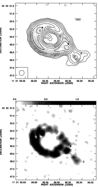
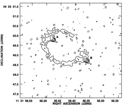
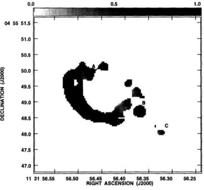
The contour levels in Figures 3.1-3.4 represent the total intensity of MG1131 at 5, 8, 15, and 22 GHz. The synthesized beam at each frequency is shown in the lower left corner. All maps display features recognized by Hewitt et al. (1988). At 5 GHz, the source consists of a radio ring, two unresolved components (A and B), and one low surface brightness extended component in the southwest direction (C). At 8 GHz, in addition to A, B, C, and the ring, a new component (D) at the center of the ring is detected. Although there is a hint of D in the 5 GHz map, it is not cleanly resolved from the ring. At 15 GHz, the surface brightnesses of C and D are below the detection limit ( 120 uJy/beam), so only A, B, and the ring are present in the map. The angular resolution at 15 GHz (0"'12) is fine enough to reveal substructures in the compact components and the ring; A and B are resolved into a possible core-jet

structure, and the ring, marginally resolved, has a gap in the northwest quadrant. At 22 GHz, only the compact components are detectable with a significant signal-to-noise ratio (> 10a, 1c = 200ttJy). The positions of the compact components in the

22 GHz map coincide with the 15 GHz peak positions of A and B.

Given the complex and extensive data reduction procedure described in Chapter 2, one might suspect that the presence of D at 8 GHz is produced solely by an artifact of the procedure. We conducted experiments to test for this possibility. Throughout the whole process, the CLEAN algorithm is the most likely source of artifacts. As a test, we created a map in which CLEAN was only permitted to

I I ... Ii I 04 55 51.5 51.0 50.5 50.0 z 0 _ o Lu a 49.5 49.0 48.5 48.0 47.5 47.0 11 0.¢ 04 55 51.5 51.0 50.5 50.0 z 0 F z 0_3i 0 Ui 49.5 49.0 48.5 48.0 47.5 47.0 11

365

31 56.55 56.50 56.45 56.40 56.35 RIGHT ASCENSION (J2000) 0 0.5 31 56.55 56.50 56.45 56.40 56.35 RIGHT ASCENSION (J2000) 56.30 1.0 56.30 56.25 56.25

Figure 3.1 - 5 GHz images. (a)Total intensity image. The contour levels are -1, 1, 2, 4, 8, 16, 32, 64, and 95% of the peak brightness of the map (19.9 mJy/beam). The vectors superimposed on the contour levels represent the electric field vectors of the polarized emission. The lengths of the vectors are proportional to the fractional polarization according to the scale shown in the upper right hand corner. The half-power contour of the beam is plotted in the lower left corner. (b) Grey-scale image of the polarized intensity ( 2/Q+ U2). The bar on the top represents the polarization intensity from 0.0 to 1.5 mJy.

I I I I I '1 I I I~)i C I I I I ·. i·, I I I _-_ I-- _-oi _{I .} i .... _ m _ _ _ _ _

04 55 51.5 51.0 50.5 50.0 49.5 0 49.0 U4 o 48.5 48.0 47.5 47.0 I I .I I I I I 11 31 56.55 56.50 56.45 56.40 56.35 56.30 56.25 RIGHT ASCENSION (J2000) 0 200 400 600 04 55 51.5 51.0 .. 50.5 50.0 ':: N. F 49.5-z 49.0 ox 48.5 48.0 -47.5 47.0 11 31 56.55 56.50 56.45 56.40 56.35 56.30 56.25 RIGHT ASCENSION (J2000)

Figure 3.2 - 8 GHz images. (a)Total intensity image. The contour levels are -1, 1, 2, 4, 8, 16, 32, 64, and 95% of the peak brightness of the map (6.7 mJy/beam). The vectors superimposed on the contour levels represent the electric field vectors of the polarized emission. The lengths of the vectors are proportional to the fractional polarization according to the scale shown in the upper right hand corner. The half-power contour of the beam is plotted in the lower left corner. (b) Grey-scale image of the polarized intensity (/Q 2+ U2). The bar on the top represents the polarization

intensity from 0 to 700 Jy.

',, _{~~~~~~~~~~~~~~~0} '@ _{':.' (} a %? :' . , I t 'by. " : vi ' -·. .... ' '~ (.~,. .. l..ooY .1 C ) OI .. I0aI I I , :: O'- I I I I a '.. 1

0 Q ° O L7 o o C? O~01~ C' ~0 o 0 .~

0~~~~~~~

a ~~0 a 0 0 B 0 I I V pB C * 0 ii . 0 0 0 A 1 I 56.50 o I oo 56.45 56.40 56.35 RIGHT ASCENSION (J2000) 31 56.55 56.50 56.45 56.40 56.35 RIGHT ASCENSION (J2000)

The contour levels are -8, 8, 16, 32,

56.30 56.25

Figure 3.4 - 22 GHz total intensity image. The contour levels are -16, 16, 32, 64, and 95% of the peak (3.8 mJy/beam).

04 55 a z 0 C z -J 0 w 0 51.5 51.0 -r 50.5 50.0 C,) 49.5 ¢ 0 49.0 o 48.5 48.0 -47.5 -47.0 I rl 0 o o 0 _O 0 0 o_oI * I I 4 I 56.30 56.25 0 o 11 31 56.55

Figure 3.3 - 15 GHz total intensity image. 64, and 95% of the peak (4.2 mJy/beam).

04 55 51.5 51.0 50.5 S 50.0 2 z 49.5 49.0 0 a 48.5 48.0 47.5 47.0 11 I I I I I I 1 . , 0 _ v ' o ,i ~~~~~~~ ' ~ 0o~~~_{o o} e , _ ooO ' - I D. o · _ ' ~~~~o O oo ' *o-. I I I I I . · - II -I