HAL Id: tel-01087024
https://tel.archives-ouvertes.fr/tel-01087024
Submitted on 25 Nov 2014HAL is a multi-disciplinary open access archive for the deposit and dissemination of sci-entific research documents, whether they are pub-lished or not. The documents may come from teaching and research institutions in France or abroad, or from public or private research centers.
L’archive ouverte pluridisciplinaire HAL, est destinée au dépôt et à la diffusion de documents scientifiques de niveau recherche, publiés ou non, émanant des établissements d’enseignement et de recherche français ou étrangers, des laboratoires publics ou privés.
plasmas : Analytical approach and in-situ data analysis
for the solar wind
Supratik Banerjee
To cite this version:
Supratik Banerjee. Compressible turbulence in space and astrophysical plasmas : Analytical approach and in-situ data analysis for the solar wind. Solar and Stellar Astrophysics [astro-ph.SR]. Université Paris Sud - Paris XI, 2014. English. �NNT : 2014PA112206�. �tel-01087024�
ÉCOLE DOCTORALE ONDES ET MATIÈRE
Laboratoire:
Laboratoire de Physique des Plasmas
Discipline:
PHYSIQUE
THÈSE DE DOCTORAT
Soutenue
le 25 septembre, 2014 par
Supratik Banerjee
Compressible turbulence in space
and astrophysical plasmas
Analytical approach and in-situ data analysis for the
solar wind
Directeur de thèse :
Prof. Sébastien Galtier (UPS, Orsay)
Composition du jury :
Président du jury : M. T. PASSOT - Directeur de recherches (Obs. de Nice) Rapporteurs : M. S. Nazarenko - Professor (Univ. of Warwick)
M. W. Schmidt - Res. Asso. (Univ. of Göttingen) Directeur de thèse : M. S. GALTIER - Professeur (Univ. Paris-Sud, Orsay)
M. F. SAHRAOUI - Chargé de recherches (LPP)
M. L. SORRISO-VALVO - Chargé de recherches (Univ. della Calabria) Membres invités: M. J. SAUR - Professor (Univ. zu Koln)
At first I would like to convey my sincere gratitude to my thesis supervisor Prof. Sébastien Galtier, my co-supervisor Dr. Fouad Sahraoui and the other honourable members of the jury for making my thesis possible and successful. I acknowledge my laboratories Institut d’Astrophysique Spatiale (IAS), Orsay and Laboratoire de Physique des Plasmas (LPP), Palaiseau for their kind co-operation.
A spacial thanks to Dr. Thierry Passot, Dr. Alexei Kritsuk, Dr. Christoph Federrath, Dr. Olivier Le contel and Dr. Lucas Sorriso-Valvo for their valuable scientific advice and encouragement. I am also grateful to the team of Prof. Vincenzo Carbone (specially Dr. Fabio Lepreti) for introducing basic methods of data analysis to me.
I am indebted to AMDA database which allowed me to use THEMIS data at free of cost and also NASA copyrighted images which were important in explaining certain aspects of my thesis.
In my thesis, I used a number of images from different sources which in-cluded journals and books subject to copyright. In this context, I would like to formally acknowledge
• American Physical Society (APS)1,
• Cambridge University Press,
• Institute of Physics (IOP publishing), • Astronomy and Astrophysics,
• Dr. Alexei Kritsuk, Dr. Thierry Passot, Dr. Annick Pouquet, Dr. Bog-dan Hnat, Dr. Chadi Salem and Dr. Lucas Sorriso-Valvo
for kindly allowing me to re-use those copyrighted images. For the other copyrighted images, the permissions are taken directly by Rightslink.
I would like to thank cordially to my friend Dr. Subimal Majee and all other friends who constantly supported me during last 3 years. A big thanks to all the members of Sammilani which is a bengali association in paris for making me happy always. I am thankful to all my friends, philosophers and guides. Finally I would like to thank all my teachers and my parents Mr. Ajit
1
"Readers may view, browse, and/or download material for temporary copying purposes only, provided these uses are for noncommercial personal purposes. Except as provided by law, this material may not be further reproduced, distributed, transmitted, modified, adapted, performed, displayed, published, or sold in whole or part, without prior written permission from the American Physical Society."
Kumar Banerjee and Mrs. Pratima Banerjee for all their contributions and sacrifices since my childhood.
I would like to acknowledge indian classical music and my guru (music teacher) Pandit Paritosh Pohankar for inspiring me at every moment.
And last but not the least ! A big thanks to my sister Indrani Banerjee and my grand mother Indira Mukherjee who always pray to god for me.
1 Introduction 1
1.1 General interest . . . 1
1.2 Turbulence in space and astrophysical plasmas . . . 2
1.3 An outline of my thesis . . . 4
2 Compressibility in fluids 7 2.1 What is compressibility ?. . . 7
2.2 Measure of compressibility for a fluid in motion . . . 9
2.3 Closure for compressible fluids . . . 11
2.4 Invariants in compressible barotropic fluid . . . 12
2.4.1 Total energy . . . 12
2.4.2 Kinetic helicity . . . 14
2.4.3 Mass and linear momentum . . . 14
2.5 Potential flow . . . 15
2.6 Two dimensional compressible flow . . . 16
2.7 One dimensional model for discontinuous compressible flow: Burgers’ equation . . . 16
2.8 Compressibility ratio for a polytropic gas across a normal shock 18 2.9 Baroclinic vector . . . 20
3 Plasma physics and magnetohydrodynamics 21 3.1 What is a plasma ? . . . 21
3.2 Two approaches to plasma . . . 23
3.2.1 Kinetic approach . . . 23
3.2.2 Fluid approach . . . 25
3.3 Magnetohydrodynamics (MHD) . . . 26
3.3.1 Mono-fluid model: Basic equations of MHD . . . 27
3.3.2 Ideal MHD approximation from generalized Ohm’s law 29 3.3.3 Linear waves in ideal MHD . . . 31
3.3.4 Invariants of ideal MHD . . . 33
3.3.5 Elsässer variables in magnetohydrodynamics . . . 38
4 Turbulent flow : important notions 43 4.1 Turbulence - A phenomenon or a theory ? . . . 44
4.2 Turbulent regime from Navier-Stokes : Reynolds number . . . 45
4.3 Chaos and/or turbulence ? . . . 48
4.4.1 Statistical homogeneity . . . 50
4.4.2 Statistical isotropy . . . 50
4.4.3 Stationary state . . . 50
4.5 Two approaches to turbulence . . . 51
4.5.1 Statistical approach . . . 51 4.5.2 Spectral approach . . . 54 4.6 Phenomenology . . . 59 4.6.1 K41 phenomenology . . . 60 4.6.2 IK phenomenology . . . 63 4.6.3 Utilities of phenomenology . . . 66
4.7 Dynamics and energetics of turbulence . . . 70
4.7.1 Turbulent forcing . . . 70
4.7.2 Turbulent cascade. . . 71
4.7.3 Turbulent dissipation . . . 73
4.8 Intermittency . . . 74
4.8.1 β fractal model . . . 77
4.8.2 Refined similarity hypothesis : Log-Normal model . . . 78
4.8.3 Log-Poisson model . . . 79
4.8.4 Extended self-similarity . . . 80
5 Turbulence in compressible fluids 83 5.1 Why is it important ? . . . 83
5.2 Primitive theoretical approaches . . . 86
5.3 Numerical approaches using one dimensional model . . . 88
5.4 Numerical Simulations in higher dimensions . . . 90
5.4.1 Numerical methods for compressible turbulence . . . . 90
5.4.2 Piecewise Parabolic Method (PPM): . . . 90
5.4.3 Compressible intermittency . . . 97
5.4.4 Compressible and solenoidal forcing . . . 99
5.4.5 Choice of inertial zone and sonic scale. . . 101
5.4.6 Two-point closure in EDQNM model for compressible turbulence . . . 102
5.5 Observational studies . . . 102
6 Exact relations in turbulence 109 6.1 Exact relations in incompressible turbulence . . . 109
6.1.1 Incompressible hydrodynamic turbulence . . . 111
6.1.2 Incompressible MHD turbulence . . . 113
6.2 Previous attempts for exact relations in compressible turbulence116 6.2.1 Heuristic approach by Carbone et al. (2009) . . . 116
6.3 New exact relations and phenomenologies in compressible
tur-bulence : My research work . . . 120
6.3.1 Isothermal hydrodynamic turbulence . . . 121
6.3.2 A new phenomenology for compressible turbulence . . 128
6.3.3 Isothermal MHD turbulence . . . 130
6.3.4 Polytropic hydrodynamic turbulence . . . 137
7 Solar wind data analysis 147 7.1 Introduction . . . 147
7.2 The solar wind . . . 148
7.2.1 The heliosphere . . . 148
7.2.2 Prediction for the solar wind . . . 149
7.2.3 The fast and the slow solar wind . . . 149
7.2.4 Exploration of the solar wind . . . 151
7.2.5 MHD fluctuations in the solar wind . . . 152
7.2.6 Nature of the solar wind turbulence . . . 152
7.3 Data source . . . 154
7.3.1 The THEMIS mission . . . 154
7.3.2 A brief description of instruments . . . 154
7.4 Judicial selection of data . . . 157
7.4.1 Selection of intervals . . . 157
7.4.2 Relevant spatial and temporal scales . . . 162
7.5 Analysis of the selected data . . . 164
8 Resuming and looking ahead... 175
8.1 Answered and unanswered issues of compressible turbulence . 175 8.2 Some future projects . . . 177
1.1 Turbulence in the mixing of milk in coffee, Credit: Daniel G. Walczyk. . . 2
1.2 Supercomputing simulation showing the formation of inter-stellar gas filaments in turbulent interinter-stellar cloud; The high-est density (red) fragments represent molecular self-gravitating cores leading to the star formation; Performed by researchers of University of California-Berkeley using the Pleiades supercom-puter at the NASA Advanced Supercomputing facility, Credit: NASA. . . 3
2.1 Highly compressible dilute diffuse gas in the interstellar space; Credit: University of Leeds. . . 8
2.2 Evolution of a Burgers’ shock in course of time (t); Credit: Ludovic Maas.. . . 18
3.1 Different types of plasmas: argon glow discharge (left above), fusion plasma (right above), uv image of solar corona (left be-low) and highly dense Lagoon nebula (right bebe-low). . . 22
3.2 Experimental verification of Alfvén waves in a hydrogen filled tube of 34 inches and of diameter 53/4 inches; The solid line
corresponds to the theoretical estimation and the circles corre-spond to the experimental values which justifies the proportion-ality of Alfvén speed to the magnetic field in an incompressible or weakly compressible fluid; The discreancy between the ex-perimental and the theoretical values are due to instrumental reasons; Reprinted with permission from (Allen et al., 1959); © (1959) American Physical Society. DOI: 10.1103/Phys-RevLett.2.383 . . . 34
3.3 Numerical simulation of twisted and knotted magnetic field lines for a system with non-zero magnetic helicity; Source: Oral presentation of Simon Candelaresi. . . 38
3.4 Order of magnitude of various plasma parameters for different types of plasmas. . . 42
4.1 Transition from laminar flow to turbulent flow as a function of increasing Reynolds number; Courtesy: Sébastien Galtier.. . . 46
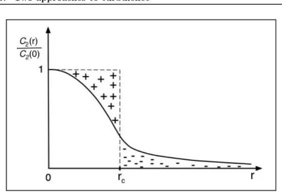
4.2 Behaviour of a second order auto-correlation function in space; Courtesy: Sébastien Galtier. . . 53
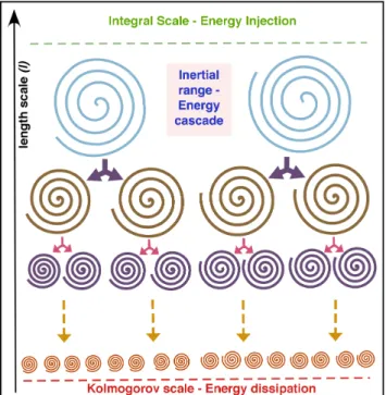
4.3 Schematic view of Richardson’s energy cascade in turbulence by eddy fragmentation. . . 60
4.4 Normalized velocity power spectra from different experiments show universal k−5/3behaviour; Reprinted with permission from
Gibson & Schwarz (1963) ; © (1963) Cambridge university press. . . 62
4.5 Sporadic interactions of Elsasser fields in IK phenomenology. 64
4.6 Clear deviation of the moments of velocity and magnetic fluc-tuations from the self-similar scaling laws of K41 and IK phenomenology in the solar wind; Reprinted with author’s permission from Salem et al. (2009); © (2009) AAS. DOI: 10.1088/0004-637X/702/1/537 . . . 75
4.7 Scaling of second order longitudinal velocity structure functions (in logarithmic plot) in time domain using data obtained from S1 wind channel of ONERA; Reprinted with permission from
Frisch (1995); © (1995) Cambridge university press. . . 77
4.8 Two dimensional representation of fractal cascade for β = 1 2;
Courtesy: Sébastien Galtier. . . 78
4.9 Comparison of different models of intermittency: plot of nth order moment for velocity structure function as a function of n, the discrete points with different colors and shapes (black and white triangles, white square, black circle and crosses) corre-spond to data obtained from different experiments, the straight chain line, dashed line, dotted line and the solid line correspond respectively the theoretical predictions of K41, beta-fractal with D = 2.8, log-Poisson and log-normal models; Reprinted with permission from Frisch(1995); © (1995) Cambridge uni-versity press. . . 81
5.1 WIND spacecraft data of velocity, density and radial magnetic field fluctuations (Days in 1995); Reprinted with permission from Meyer-Vernet (2007) ; © (2007) Cambridge university press. . . 84
5.2 Total mechanical energy spectra (left); step discontinuities for turbulent density and triangular discontinuities for turbulent velocity field (right); Source: Tokunaga (1976).. . . 89
5.3 PDF of s = lnρ for (i) isothermal case (left), (ii) γ < 1 (right-upper) and (iii) γ > 1 (right-lower) for one dimensional gas turbulence; Reprinted with permission from Passot & Vazquez-Semadini (1998); © (1998) American physical society. DOI: 10.1103/PhysRevE.58.4501 . . . 91
5.4 Vortex structures in numerical simulation (using PPM) of two dimensional compressible turbulence with 5122 resolution (left)
and power density spectra (right) for (i) solenoidal kinetic en-ergy (ES) (solid line), (ii) compressible kinetic energy (EC)
(dashed line) and (iii) total kinetic energy (Ev) (dotted line);
Reprinted with permission from Passot et al.(1988); © (1988) ESO. . . 92
5.5 Power density spectra for (in logarithmic graph) (i) solenoidal kinetic energy (ES), (ii) compressible kinetic energy (EC) and
(iii) total kinetic energy (Ev) in three dimensional compressible
turbulence PPM simulation with 2563 resolution; the solenoidal
and the total kinetic energy spectra follow a k−0.95 law whereas
the compressible kinetic energy spectrum follows a steeper k−1.8 law; Reprinted with permission from Porter et al. (1992);
© (1992) American Physical Society. DOI: 10.1103/Phys-RevLett.68.3156 . . . 93
5.6 Power density spectra for (i) solenoidal kinetic energy (ES)
(left above), (ii) compressible kinetic energy (EC) (left below)
using 643 (Q40), 1283 (Q41), 2563 (Q42) and 5123 (Q43) grid
points and (iii) vortex tube structures in 5123 numerical box of
supersonic turbulence (right); Reprinted with permission from
Porter et al. (1994); © (1994) AIP publishing LLC. . . 94
5.7 Projected gas density of Mach 6 turbulence PPM simulation with 20483 resolution. White, blue and yellow colors
repre-sent respectively low, intermediate and high projected density values; Reprinted with author’s permission from Kritsuk et al.
(2009). . . 95
5.8 Power density spectra corresponding to (a) total velocity (v), (b) solenoidal velocity (vs), (c) compressional velocity (vc), (d)
ρ1/2v and ρ1/2v
s, (e) w ⌘ ρ1/3v and (f) ρ; Reprinted with
per-mission from Kritsuk et al. (2007a); © (2007) AAS. DOI: 10.1086/519443 . . . 96
5.9 Scaling of third order structure functions of w ⌘ ρ1/3v using
data of three dimensional supersonic turbulence (r.m.s. Mach ⇠ 6) with 10243 resolution; Reprinted with author’s permission
from Kritsuk et al. (2007b). . . 98
5.10 Compensated power density spectrum of w ⌘ ρ1/3v using data
of three dimensional supersonic turbulence (r.m.s. Mach ⇠ 6) with 20483 resolution; Reprinted with author’s permission from
5.11 Compensated power spectra corresponding to different vari-ables using solenoidal and compressible forcing; Reprinted with permission from Federrath et al. (2010); © (2010) ESO. . . . 100
5.12 Modified interpretation of power spectra with the newly defined sonic scale; Reprinted with permission from Federrath et al.
(2010); © (2010) ESO. . . 101
5.13 Solenoidal and dilatational velocity power spectra for different turbulent Mach numbers at large times (left) and Pressure spec-tra at different time instants (right) obtained using EDQNM model for weakly compressible turbulence; Reprinted with per-mission from Bertoglio et al.(2001); © (2001) AIP publishing LLC. . . 103
5.14 Moments of proton density fluctuations and magnetic field mag-nitude fluctuations as a function of the order of moments in slow (left) and fast (right) solar wind; Reprinted with permission from Hnat et al. (2005); © (2005) American Physical Society. DOI: 10.1103/PhysRevLett.94.204502 . . . 105
5.15 Compressible and incompressible scaling (in log-log graph) in time domaine of the fast solar wind data obtained from Ulysses spacecraft, Y± W± represent respectively the incompressible
and compressible third order moments; Reprinted with permis-sion from Carbone et al. (2009); © (2009) American Physical Society. DOI: 10.1103/PhysRevLett.103.061102 . . . 106
5.16 Heating energy supply by compressible pseudo-energy ε± I
dis-sipation (Red and Blue squares) and incompressible pseudo-energy ε±
I dissipation (Green and Violet circles) in comparison
with two theoretical estimations of the radial temperature pro-file for fast solar wind; Reprinted with permission from Car-bone et al. (2009); © (2009) American Physical Society. DOI: 10.1103/PhysRevLett.103.061102 . . . 107
6.1 Dilatation (left) and compression (right) phases in space cor-relation for isotropic turbulence. In a direct cascade scenario the flux vectors (blue arrows) are oriented towards the center of the sphere. Dilatation and compression (red arrows) are ad-ditional effects which act respectively in the opposite or in the same direction as the flux vectors. . . 125
6.2 Numerical verification of scaling (logarithmic plot) of the flux (F ) and the source terms (Q) of equation (6.55) in supersonic turbulence using 10243 resolution; Reprinted with permission
6.3 Phenomenological view of compressible MHD turbulence in the presence of a strong directive magnetic field; An axisymmetric total energy cascade is predicted in the perpendicular direc-tion of the strong directive magnetic field following the same phenomenology of the hydrodynamic case; Source: Banerjee & Galtier(2013). . . 137
7.1 A schematic figure of the heliosphere; Credit: NASA. . . 149
7.2 Solar wind speed and the magnetic field polarity observations from the Ulysses spacecraft covering almost all the latitudes from the equatorial to the polar region; Reprinted with per-mission from Biskamp(2008); © (2003) Cambridge university press.. . . 150
7.3 An artist view of the five spacecraft of the THEMIS mission; Credit: NASA. . . 153
7.4 Working principle of the fluxgate magnetometer (FGM). . . . 155
7.5 A schematic view of ESA; Credit: Barkeley. . . 157
7.6 THEMIS spacecraft with its onboard instruments; Credit: NASA and oral presentation of Le Contel et al. . . 158
7.7 THEMIS spacecraft orbits during different periods; the red tra-jectory corresponds to THEMIS B and the grey region repre-sents the solar wind; Credit : http://themis.ssl.berkeley.edu/ . . . 159
7.8 Spacecraft trajectories (red line) obtained by SSC Orbit Viewer along with the positions of the magnetopause (off-white net like region) and bow-shock (green net like region). D1x, D2x,
D3x represent respectively the distance of the spacecraft from
the Earth, the magnetopause and the bow-shock along the x-direction. . . 160
7.9 Examination of the ionic fluid temperature for a 24-hour inter-val on 14/07/2008-15/07/2008. . . 161
7.10 Selection of Fast solar wind data for the periods of 15/06/2008 - 10/10/2008 and 15/06/2009 - 10/10/2009, the three compo-nents of velocity (in km/s) are given in three different colors (as explained in the image). . . 161
7.11 The fluctuation data scheme of 8h-11h of 11/08/2008 obtained from AMDA - the ion velocity components, ion density and magnetic field components are given in the respective three panels (top figure); calculated density fluctuations (in green) about the mean value (in violet) (middle panel) and the scaling of incompressible (in red) and partial compressible flux (in blue) as a function of time lag τ (bottom panel). . . 165
7.12 (a) Interval with negative incompressible and compressible flux, (b) Interval with positive incompressible and compressible flux. 167
7.13 (c) Interval with positive incompressible flux and negative com-pressible flux, (d) Interval with negative incomcom-pressible flux and positive compressible flux. . . 168
7.14 The effect of compressibility on the discrepancy between the incompressible and compressible flux. . . 169
7.15 Almost constant plasma beta parameter of order unity during a 10 hour interval of 10/08/2008 -11/10/2008 (second panel) . 170
7.16 Comparison of incompressible (in black), heuristic compressible (in green) and analytical compressible (in red) scalings in a 6-hour interval of 2008 . . . 172
7.17 Comparison of incompressible (in black), heuristic compressible (in green) and analytical compressible (in red) scalings in a 6-hour interval of 2009 . . . 172
4.1 Self-similarity with K41 phenomenology. . . 76
4.2 Self-similarity with IK phenomenology. . . 76
5.1 Different power spectra in supersonic turbulence (Kritsuk et al.,
2007a).. . . 95
7.1 Selected intervals of the fast solar wind with continuous data set162
7.2 Average values of the flux terms (for 3 s. lag) for a number of three-hour intervals . . . 171
Introduction
Contents
1.1 General interest . . . 1
1.2 Turbulence in space and astrophysical plasmas . . . . 2
1.3 An outline of my thesis . . . 4
1.1 General interest
T
urbulencephysics. In a simplistic manner, one can describe turbulence as a veryis said to be one of the last unsolved problems of classicalcomplicated non-linear fluid flow principally associated with vortices. It is easier to describe turbulence than to analyze it. Till date, no satisfactory analytical theory has been established to understand turbulence. It is even obscure to determine the suitable approach for understanding turbulence. De-spite this enormous complexity, the most intriguing feature of turbulence is its ubiquity in nature. Starting from the everyday fluids like tap water or milk in a cup of hot coffee (see fig. 1.1), prominent signatures of turbulence are observed in the tropospheric air, the space plasmas (the solar wind, magne-tospheric plasmas) and even in the interstellar clouds which give birth to the stars. Other than the usual hydrodynamical fluids and plasmas, turbulence is believed to describe various phenomena in non-linear optics (Garnier et al.,
2012), small scale biological fluids like microbial suspensions (Wensink et al.,
2012). Turbulence is also observed in quantum mechanics (Proment et al.,
2009). Most interestingly, turbulent behaviour is significantly perceived even in the field of finance and economics. This fact can be justified by a famous remark of Benoit Mandelbrot, who said
" The techniques I developed for turbulence, like weather, also apply to the stock market."
The formal study of turbulence is evoked from some practical interests. One of them is its efficiency in mixing. A spoon of milk gets uniformly mixed in coffee within some seconds only if we stir it to create turbulence.
Without turbulence the mixing would take place by pure molecular diffusion and would take several months to be completed. In case of weather forcasting,
Figure 1.1: Turbulence in the mixing of milk in coffee, Credit: Daniel G. Walczyk.
an understanding of turbulence is a must. The first theories of turbulence were indeed born out of that very interest (Richardson, 1922). Moreover, a thorough investigation of atmospheric turbulence or more precisely clear air turbulence (CAT) could be useful for reducing hazards to aircraft passengers across the zones of rough air and also to design more efficient aircrafts.
1.2 Turbulence in space and astrophysical
plas-mas
Clear signature of turbulence has been observed (Armstrong et al., 1995;
Bruno & Carbone, 2005) also in the space plasmas like solar wind, magneto-spherical plasmas etc. and in the astrophysical plasmas. In several studies it is observed that the fluctuations in the aforesaid plasmas usually associate large number of spatial and temporal scales and the power spectrum of energy follows almost an identical power law (with index -5/3) to the one predicted by Kolmogorov for incompressible hydrodynamic turbulence (discussed in de-tails in chapter 4). However, the plasma turbulence is not exactly identical to ordinary fluid turbulence due to the presence of electromagnetic fields.
Moreover, the space plasmas are usually non-collisional and hence a viscous dissipation mechanism cannot be associated. One has thus to consider the plausibility of kinetic turbulence in such plasmas (Belmont et al., 2014). In case of the solar wind, low frequency fluctuations are modelled by ordinary MHD turbulence whereas more sophisticated models like Hall MHD, electron MHD or purely kinetic approaches are needed to explain high frequency fluc-tuations (Meyrand & Galtier, 2010; Salem et al., 2012). An understanding of solar wind turbulence is necessary in order to understand the acceleration and the anomalous heating of solar wind (Tu & Marsch, 1997). In course of this thesis, analytical studies along with some spacecraft data analysis have been performed in order to address these issues. On the other hand, turbu-lence in the cold molecular highly compressible interstellar clouds is believed to bring about the formation of a star by preventing the collapse of a self-gravitating cloud. The scientists of University of California-Berkeley have recently performed large scale supercomputing simulations (see figure1.2) for understanding the underlying mechanisms.
Figure 1.2: Supercomputing simulation showing the formation of interstel-lar gas filaments in turbulent interstelinterstel-lar cloud; The highest density (red) fragments represent molecular self-gravitating cores leading to the star for-mation; Performed by researchers of University of California-Berkeley using the Pleiades supercomputer at the NASA Advanced Supercomputing facility, Credit: NASA.
1.3 An outline of my thesis
Compressibility in fluids is a non trivial issue which becomes more complicated when discussed in the framework of turbulence1. The principal work of my
thesis consists of deriving analytical statistical constraints or so-called exact relations for compressible turbulence. A clear theoretical background is thus necessary to be developed before presenting my work. Besides, the subject of my thesis largely covers fluid mechanics, plasma physics and also space physics. The composition of this thesis is accomplished from a pedagogical point of view so as to render it accessible to all the persons having knowledge of at least one of the three domains. Besides, discussing the main problematic of the thesis, parallel attempts are also taken to address some misconceptions or unanswered issues in a more general context. Including this introduction, this thesis consists of eight chapters.
In the second chapter of this thesis, different concepts and measures of compressibility have been introduced in a general context for a neutral fluid. Some simple thermodynamic closures (polytropic, barotropic etc.) have been discussed along with the associated inviscid invariants (mass, linear momen-tum, total energy and kinetic helicity). Very familiar one dimensional model of Burgers (1948) is also discussed including some properties of shock waves in a compressible flow.
The third chapter presents a brief overview of plasma physics. The re-ductions of kinetic Boltzmann equations2 into fluid equations and finally into
monofluid Magnetohydrodynamic (MHD) equation have been worked out in a detailed manner. The approximation of ideal MHD, the corresponding lin-ear wave modes (Alfvén and magnetosonic modes) and integral invariants (mass, total energy, cross-helicity, magnetic helicity etc.) are discussed in a schematic way. The notions of Elsässer variables and pseudo-energies both in incompressible (Elsässer,1950) and compressible MHD (Marsch & Mangeney,
1987) have been introduced at the end of the chapter.
The fourth chapter is dedicated to introduce turbulence or rather incom-pressible turbulence both in neutral and MHD fluids. The chapter begins with some interesting debatable issues like the proper definition of turbulence or the distinction between chaos and turbulence. This part is followed by a schematic discussion of different statistical symmetry considerations in the study of turbulence. The notions of correlation functions, structure functions
1
The construction of the sentence was done deliberately in order to present an alternative point of view than the usual one where we say that turbulence in fluids is complicated and becomes more complicated in compressible fluids.
2
In usual books, the fluid equations are derived from collisionless Vlasov’s equation which is physically not correct.
and energy power spectra have been elucidated always in incompressible tur-bulence. With all these elements two different phenomenological views K41 and IK are described respectively for hydrodynamical and magnetohydro-dynamic turbulence along with the corresponding power laws which predict respectively a −5/3 and a −3/2 power law index for the energy power spectra. The dynamics and the physics of energy cascade in turbulence are explained using those phenomenological views. Finally, the aspect of self-similarity or the scale invariance in turbulence is investigated using different models of intermittency and also a slightly different notion of extended self similarity (ESS). This chapter practically sets up the theoretical background for present-ing my thesis work thereby renderpresent-ing the later more accessible to someone who is not very familiar to the fundamentals of turbulence.
The fifth chapter contains a very brief review of different types of research works which have been accomplished in exploring the fundamental properties of compressible turbulence upto the beginning of my thesis and have played some role in conglomerating my ideas over compressible turbulence and possi-ble scopes in that said field. Some initial theoretical approaches are discussed along with their predictions in a separate section. This part is followed by another discussion of some important numerical approaches in compressible turbulence and their different predictions in physical space and Fourier space scaling. High resolution numerical simulations (Kritsuk et al., 2007a,b; Krit-suk et al.,2010;Federrath et al.,2010) employing piecewise parabolic method (PPM) for supersonic turbulence are discussed in an elaborate way. Unlike incompressible turbulence, no −5/3 power law is found for the fluid velocity power spectrum for compressible fluids. However, the Kolmogorov type −5/3 spectrum is found to be recovered even in compressible turbulence if one con-siders the power spectra for cube-root density weighted velocity instead of normal fluid velocity. For the MHD turbulence simulations, an identical sit-uation is noticed for the Elsässer variables. A theoretical rather analytical explanation for this behaviour is tried to investigate in scope of my thesis. The chapter ends with some significant research works on the compressible turbulence in astrophysical plasmas and space plasmas. Specially the work of
Carbone et al. (2009) using Ulysses spacecraft data revealed significant im-provement in fast solar wind turbulence scaling laws when density fluctuations are taken into account and also hints at the importance of a cube-root density weighted velocity variable in compressible turbulence.
The sixth chapter comprises of my research works on compressible turbu-lence. It begins with the derivations of some exact relations in incompressible hydrodynamic and MHD turbulence. After describing some shortcomings of previous theoretical approaches in compressible case, we have derived our ex-act relations for (a) isohtermal neutral fluid (Galtier & Banerjee, 2011), (b)
isothermal MHD fluid and (Banerjee & Galtier, 2013) (c) polytropic neutral fluid (Banerjee & Galtier, 2014). With each derivation, we have tried to understand the corresponding phenomenology and thereby predicting some spectral indices. Interestingly, the justification behind the scaling of density weighted velocity becomes clearer owing to these relations. Although the aspect of anisotropy is beyond the scope of my thesis, a simple anisotropic phenomenology is proposed in compressible MHD turbulence in the presence of a very strong mean or external magnetic field. In case of polytropic turbu-lence, fluctuations of local sound speed and the algebraic value of polytropic index are predicted to play an important role.
In the chapter 7, a brief but formal introduction of the solar wind is given. The applicability of MHD in case of the large scale fluctuations are also dis-cussed. The following part is dedicated to test our exact relation for com-pressible MHD turbulence using the THEMIS spacecraft data. After giving a very brief introduction of the THEMIS mission and some of its instruments, a step-by-step description of the data selection process is provided. In case of fast solar wind, incompressible scaling is compared with the compressible scal-ing whence an attempt to quantify the compressibility in the fast solar wind turbulence is taken. All these studies in case of slow solar wind are kept as future projects in order to compare the role of compressibility between these two types of winds.
Finally, in the chapter 8, the significance of my work is resumed briefly along with some unanswered issues. The chapter ends with a list of propositions of future works both in theory of compressible turbulence and in spacecraft data analysis of the space plasmas.
Compressibility in fluids
Contents
2.1 What is compressibility ? . . . 7
2.2 Measure of compressibility for a fluid in motion . . . 9
2.3 Closure for compressible fluids . . . 11
2.4 Invariants in compressible barotropic fluid . . . 12
2.4.1 Total energy . . . 12
2.4.2 Kinetic helicity . . . 14
2.4.3 Mass and linear momentum . . . 14
2.5 Potential flow . . . 15
2.6 Two dimensional compressible flow . . . 16
2.7 One dimensional model for discontinuous
compress-ible flow: Burgers’ equation . . . 16
2.8 Compressibility ratio for a polytropic gas across a
normal shock . . . 18
2.9 Baroclinic vector . . . 20
2.1 What is compressibility ?
C
ompressibilitymeasure of ease with which its density can be altered either locally orof a matter (solid, liquid or gas) can be described as aglobally. So, in a sense compressibility is inverse to the elasticity of a material. An increase in density (for a given mass) with respect to an initial density corresponds to lower volume with respect to the initial volume and is called compressionwhereas a decrease in density and hence a rise in volume is known as rarefaction or dilatation.
The solids are highly elastic and very hard to deform. Their compressibility is very low. The liquids are a bit less elastic but the compressibility is very low too. Compressible fluid family is primarily represented by gases. They
are usually very easy to be compressed or rarefied i.e. for a given pressure change a gas will respond the best in comparison with solids and liquids (which are almost indifferent to it). Formally compressibility (β) is defined as the inverse of bulk modulusi.e. the fractional change in volume for unit change in pressure (for a given temperature T) and is written as
β = 1 V ✓ ∂V ∂P ◆ T . (2.1)
It is important to note that the compressibility of a material is a function of instantaneous temperature and pressure (Fine & Millero,1973). Typically, at 273 K, the compressibility of water is 5.1 ⇥ 10−10 P a−1 in the neighbourhood
of zero pressure. Under the same condition, the compressibility of air is about 10−5 P a−1 which shows that air is much more compressible than water. The
Figure 2.1: Highly compressible dilute diffuse gas in the interstellar space; Credit: University of Leeds.
above discussion, however, is appropriate for a solid or liquid or gas in static condition. If we study a fluid in motion, then we have two points of view for
studying the fluid. The first one is Lagrangian view which consists of studying the flow by following a fluid blob (of given mass) and recording the changes of different dynamical variables in course of time. Compressibility of the fluid here is presented by the variation of density of the given blob with time. In order to use the other one which is Eulerian point of view, a fixed geometric volume in space is considered and the dynamical variables at each space and time point in that volume are studied. In this context compressibility is said to exist if the density functions (ρ(x, t)) have a non-zero temporal or spatial derivative almost everywhere.
2.2 Measure of compressibility for a fluid in
mo-tion
Unlike the static case, it is difficult to give a consistent measure of compress-ibility for a fluid in flow. It is because in the second case the compresscompress-ibility is no more a pure material property but gets influenced by the corresponding flow dynamics. We thus talk of compressible flow. The basic dynamical equations for a neutral (without charge) fluid is given by
∂ρ ∂t + r · (ρv) = 0, (2.2) ∂v ∂t + (v · r) v = − rP ρ + f + ν∆v + ν 3r (r · v) , (2.3) where v (x, t) is the Eulerian fluid velocity, P (x, t) is the fluid pressure, f is the body force per unit mass and ν is the kinematic viscosity (which is the ratio of dynamic viscosity to the fluid density). For an incompressible flow, at each point (x, t) of the flow field, density is constant and the above two equations get reduced to
r · v = 0, (2.4)
∂v
∂t + (v · r) v = −rP + f + ν∆v. (2.5) It is however noteworthy that in Eulerian case, the condition (2.4) is an out-come of incompressibility and not necessarily imply incompressibility (one can check immediately) whereas it corresponds directly to Lagrangian incompress-ibility. Throughout our discussion, we shall consider the Eulerian point of view.
Despite its difficulty, it is important to have a measuring parameter to com-pare the degree of compressibility of different fluid flows so that the effect of
compressibility on different phenomena can be analyzed easily. In the fol-lowing we try to construct a quantity which can be a consistent measure of compressibility. We assume an ideal (no viscosity) fluid which was initially at rest with uniform initial density ρ0 and not necessarily uniform initial pressure
P0. The initial pressure gradient is equal to the body force (which is
indepen-dent of the flow) thereby producing zero acceleration. Now we assume very small perturbation in density ρ1(⌧ ρ0) which causes small perturbations in
velocity (which was initially zero) and pressure and are respectively given by vand P1. The non-linearity, consisting of terms which are negligible with one
order higher, does not contribute to the modified dynamics and so we are left with ρ0 ∂v ∂t + rP1 = 0, (2.6) ∂ρ1 ∂t + ρ0r · v = 0. (2.7) Assuming plane wave solution for the perturbations, we obtain simply
ω2 f = ✓ P1 ρ1 ◆ k2 = C2 Sk2, (2.8)
where ωf and k denote respectively the angular frequency and the
wavenum-ber of the linear mode(s). The above equation shows that one mode is possible and that can easily be identified to acoustic mode (or sound wave) with phase velocity (and group velocity) equal to CS =pP1/ρ1. Hence we can conclude
that any small perturbation in a compressible ideal fluid can propagate with sound speed. Alternatively speaking, any information of small density fluc-tuation can be propagated between two points with mutual separation l in a characteristic compressible time τC = l/CS. For an incompressible fluid,
CS is infinity and so τc = 0. We can hence argue that higher the τC, higher is
the compressibility of the fluid. Following the same reasoning, we can say that for a given flow with velocity v(x, t), a reliable measure of its compressibility can be given by the dimentionless ratio | v |/CS which is known as the local
Mach number of the flow and is denoted by M(x, t). So for small density per-turbation, the supersonic flow is more compressible than a subsonic flow and the compressibility is linear with the Mach number according to our present method. This formalism is done for ideal fluid. The insertion of viscosity cannot, however, alter the propagation speed but attenuates the amplitude of the wave.
Another approach for measuring the compressibility is by the method of Helmholtz decomposition (Helmholtz, 1867). We learnt previously that incompressible fluid velocity is solenoidal or divergenceless (2.4). Helmholtz
decomposition expresses the fluid velocity vector, in general case, as a vector sum of two components - i) Solenoidal part (vS) and ii) Compressible part
(vC)where by definition, r · vS = 0 and r ⇥ vC = 0. A possible measure for
compressibility can be given simply by the ratio | vC |/| vS |. By construction,
these two components are mutually orthogonal in Fourier space as
k · ˆvS = 0 ; k ⇥ ˆvC = 0. (2.9)
This fact enables us to decompose the velocity in longitudinal (parallel to k) and transverse components (ˆvS and ˆvS respectively) in Fourier space.
In the community of turbulence, however, some different quantities are used to quantify the influence of compressibility in a turbulent fluid. The simplest one can just be given as | r · v |/| r ⇥ v | which is approximately analogous to the last definition using Helmholtz decomposition. Another measure is obtained from the so-called small scale compressive ratio (rCS) (Kida &
Orszag,1990,1992; Kritsuk et al., 2007a) which is given by
rCS = ⌦| r · v |
2↵
⌦| r · v |2
↵ + ⌦| r ⇥ v |2↵ , (2.10) and is believed to reflect the compressible effects in length scales near the viscous length scale in a turbulent fluid. In their paper, Federrath et al.
(2010) used another slightly different version. In order to quantify the relative importance of compressive motion over rotational motion, they used the ratio EC(k)/Etot(k) where the numerator and the denominator are defined as
Z 1 0 EC(k)dk = 1 2 Z 1 0 ˆ vC· ˆv⇤C4πk2dk, Z 1 0 Etot(k)dk = 1 2 Z 1 0 ˆ v · ˆv⇤4πk2dk.
A simple measure of compressibility can also be obtained by the quantity ρ1/ (ρ0P1) which reflects the static case but this measure does not take into
account the flow velocity and hence does not consider the correlation between the compressibility and the kinetics.
2.3 Closure for compressible fluids
As shown in the previous section, the basic equations for a hydrodynamic fluid consist of the mass continuity equation and the momentum conservation equation which get a simpler form (2.4 and 2.5) for an incompressible fluid.
These two equations (in fact four equations, the second being a vector equa-tion) form a closed system1. Precisely speaking, we have one vector variable
v and one scalar variable P (of course it is a simplification for an isotropic fluid otherwise P would be a tensor of rank two) - and we have one vector equation and a scalar one. For compressible fluids, density appears to be an additional scalar variable. So we need another scalar type relation in order to close the system. A usual practice is to express the fluid pressure as a function of fluid density. The corresponding fluid or flow-field is known as barotropic fluid. A more simplified closure is obtained if we express the fluid pressure proportional to an arbitrary power law of the density i.e.
P = Kργ.
This type of closure is called polytropic closure. Depending on the values of γ, we have the following cases. The case γ = 1 corresponds to isothermal case where the proportionality constant K comes to be the square of sound speed of the flow field. γ = cp/cv is the adiabatic closure, where cp and
cv denote respectively the specific heat of a fluid at constant pressure and in
constant volume. For γ = 0 we get an isobaric fluid where the fluid pressure is constant throughout. Incompressible limit can be derived from this polytropic closure if γ −! 1 and can be shown as follows:
∂t(P ρ−γ) = 0 ) ∂tP + v · rP + γP (r · v) = 0. (2.11)
The limit γ −! 1 leads to the condition r · v = 0 which represents an incompressible flow.
Another possible closure may be the irrotationality of the flow which means r ⇥ v = 0, although this is a vector closure and cannot readily be applied to serve our purpose.
For the flow field where energy transport is important, we have to go further and write the evolution equation for temperature too. Then for closing the system, we have to use some closure relating heat flux, pressure, density etc.
2.4 Invariants in compressible barotropic fluid
2.4.1
Total energy
In general for three dimensional compressible flows whose dynamics is gov-erned by the Navier-Stokes equations, the total energy is a conserved quantity
1
In the present context, the concept of closure is used in a view to having a closed system of algebraic equations obtained after having linearized the fluid equations which themselves cannot be closed so easily due to the non-linearity in the Navier-Stokes equations.
if the viscosity of the fluid is neglected (inviscid case). This fact is an imme-diate consequence of translational symmetry in time of inviscid Navier-Stokes equations. If the system of equation is closed with a barotropic closure i.e. P = P (ρ) we can show that the total energy density is given as
E = ρ v 2 2 − Z P d✓ 1 ρ ◆( = ρ v 2 2 + Z Pdρ ρ2 ( .
One can easily identify that the above expression consists of two terms - kinetic energy and compressive internal energy. The internal energy per unit mass is formally defined as e = − R P d (1/ρ). The total energy conservation is shown below. First we have :
∂R Edτ ∂t = Z ∂E ∂tdτ = Z ∂ ∂t ρv 2 2 − ρ Z P d✓ 1 ρ ◆( dτ. (2.12) Now we show that (using elementary vector calculus identities)
∂ ∂t ✓ ρv 2 2 ◆ =✓ v 2 2 ∂ρ ∂t + ρv · ∂v ∂t ◆ = −r · ✓ ρv 2 2 v ◆ − v · rP (2.13) and −∂ ∂t ✓ ρ Z P d✓ 1 ρ ◆◆ = −er · (ρv) +1 ρ ∂ρ ∂t ∂ ∂⇣1⇢⌘ Z P d✓ 1 ρ ◆( = −er · (ρv) − Pρr · (ρv) = −er · (ρv) − P (r · v) − Pρv· rρ. (2.14) We note further that
ρv · re = −ρv · r Z P d✓ 1 ρ ◆( = −ρv · P r✓ 1ρ ◆ = P ρv· rρ. (2.15) Using (2.13), (2.14) and (2.15), we obtain
∂E ∂t = −r · ✓ ρv 2 2v+ ρev + P v ◆ = −r · F. (2.16) The above equation has the conservative form. The rate of change of total energy density equals to the divergence of flux F. Using Gauss’ divergence theorem and assuming that the normal component of the flux vanishes at the boundary surface of our chosen volume, we can show that the total energy ,R Edτ- is an inviscid invariant in three dimensional compressible flow.
2.4.2
Kinetic helicity
Kinetic helicity is a pseudo scalar and is defined as R H!dτ where H! = v · ω
and ω = r ⇥ v is the vorticity vector. The introduction of kinetic helicity was also thanks to Helmholtz decomposition (Wu et al.,2007) discussed above. The velocity vector as well as the vorticity vector can be decomposed in lateral and transverse components with respect to one another and can be written as v2ω = H!v+ v ⇥ Λ, (2.17) ω2v= H!ω− ω ⇥ Λ, (2.18) where the longitudinal and transverse components of velocity and vorticity are respectively proportional to the kinetic helicity density H! and the vector Λ
called the Lamb vector. In case of an inviscid barotropic fluid (under possible conservative body force) total kinetic helicity is a conserved quantity thereby describing the frozen vortex lines in the flow and hence a conservation of the number of linkage or knottedness of those lines within them (Thomson,1869). Here, in the following, we examine the conservation of kinetic helicity of an inviscid barotropic fluid :
∂H! ∂t = ∂v ∂t · ω + ∂ω ∂t · v (2.19) = − (v · r) v − rP (ρ)ρ ( · ω + [r ⇥ (v ⇥ ω)] · v (2.20) = −r ·✓ v 2 2ω ◆ −rP (ρ) ρ · ω + r · [v ⇥ (v ⇥ ω)] . (2.21) In the step (2.20), we have used the fact that for a barotropic fluid, the baroclinic vector (rP ⇥ rρ) is always zero. The expression (2.21) however does not guarantee the conservation of kinetic helicity. Under the condition where the rP/ρ can be written as a pure gradient, (2.21) is reduced to a pure divergence form thereby guaranteeing the conservation of total kinetic helicity under the assumption that either the corresponding flux vector disappears at every point on the flow-field boundary surface or at the boundary surface it is purely tangential to the surface. Fortunately, the usual closures of type polytropic (non-isothermal) (P = Kργ) or isothermal (P = C2
sρ) satisfies the
necessary condition for kinetic helicity conservation in a compressible flow.
2.4.3
Mass and linear momentum
The above two conservations are non-trivial and they are not in general avail-able (as they are derived here) in the text-books. For the total mass ,R
ρdτ-and the total linear momentum ,R ρvdτ- conservation, the demonstration is more or less trivial and can immediately be obtained respectively from equa-tions (2.2) and (2.3). Is it noteworthy that these two quantities are conserved even in the presence of finite fluid viscosity. The conservation of linear mo-mentum (as one can expect) is a direct consequence of the absence of any net external force on the system whereas the mass conservation shows that the fluid flows in a closed system which prohibits any mass exchange with the exterior.
2.5 Potential flow
In the above section we have presented the irrotationality (r ⇥ v = 0) as a closure. But the significance of irrotationality is deeper than that and re-presents a specific class of flow which is known as potential flow. The basic reason behind the name resides in the fact that for an irrotational fluid, the flow velocity vector can be expressed as a gradient of a scalar potential φ i.e. v = −rφ (Zakharov & Sagdeev,1970). If the fluid is additionally incompress-ible then the potential satisfies Laplace’s equation i.e. ∆φ = 0. The flow can be determined just by its kinetics (no information on the dynamics i.e. the applied force is required to determine the local velocity field). An important field of application for the potential flow is compressible flows. Remembering the Helmholtz’s equation, we can understand that the flow velocity has only its compressible part which means v ⌘ vC and vS = 0 and thus such a fluid
is infinitely compressible according to our measure of compressibility using Helmholtz decomposition.
For this type of flow, the kinetic helicity is trivially conserved as it is iden-tically zero (ω = 0) in this case. Interestingly for an irrotational inviscid fluid the baroclinic vector is also identically zero. The fact can easily be verified by taking the curl of (2.3) omitting the viscous and the forcing term. It is thus concluded that a barotropic fluid need not be, in general, irrotational but an irrotational fluid necessarily implies barotropicity when the viscosity is ne-glected. The total energy is thus always conserved by the virtue of 2.4.1. In the following, we shall search for the conservation of the total fluid dilatation i.e. R (r · v) dτ.
Throughout our study, we have searched for flow invariants in the inviscid limit in the absence of any net external forcing. This very procedure, although not general, is appropriate in the framework of our study of completely de-veloped turbulence in the inertial zone - a zone which is supposed to be independent of the external forcing and the small scale viscous effects. A de-tailed discussion on this point will be done later while introducing the fluid
turbulence and its different aspects.
2.6 Two dimensional compressible flow
Discussion over two dimensional flows builds an essential part of fluid dynam-ics owing to its numerous practical applications. It is however a bit tricky to talk about the two dimensional flows. The number of available spatial coordi-nates are three but the fluid velocity vector is spanned in two dimensions and any variation in the third dimension is neglected. This type of flow field are thus sometimes called 2.5 dimensional. The velocity field is assumed to be in x-y plane (by choice) and is defined as
v= vx(x, y)ex+ vy(x, y)ey, (2.22)
and the gradient operator is defined as r ⌘ ∂
∂xex+ ∂
∂yey. (2.23)
The corresponding vorticity vector (pseudo-vector to be precise) is then de-fined as ω = r ⇥ v =✓ ∂vy ∂x − ∂vx ∂y ◆ ez = ωez. (2.24)
This above construction makes the kinetic helicity density (v · ω) identically zero (v ? ω) everywhere in the flow field. The total kinetic helicity is thus trivially conserved irrespective of the closure of the fluid. An interesting fam-ily of invariants has been obtained for two dimensional flow of a barotropic, inviscid fluid by Pedlosky (1987). These invariants are function of a newly defined quantity called potential vorticity (ωρ = ω/ρ). Using eqn. (2.2)
and taking the curl of the eqn (2.3), we can show that in the inviscid limit, for a three dimensional flow we have
∂ω⇢
∂t + (v · r) ω⇢ = (ω⇢· r) v. (2.25) By the above construction, we obtain additionally for a two dimensional flow (ω⇢· r) = 0, which renders ω⇢ to be a Lagrangian invariant or material
invariant of the flow.
2.7 One dimensional model for discontinuous
compressible flow: Burgers’ equation
From the above discussion, we can understand that for compressible fluids we cannot derive any separate evolution equation for the velocity field right
from the Navier-Stokes equations. However, if we consider a compressible flow in one dimension, there exists a simplistic yet very useful scalar evolution equation for the fluid velocity field - this equation is called Burgers’ equation after J. M. Burgers who played an essential role in popularizing this equation in the framework of compressible turbulence (Burgers, 1948). The equation is written as ∂v ∂t + v ∂v ∂x = ν ∂2v ∂x2. (2.26)
This equation was known to the mathematicians and physicists well before Burgers. Burgers’ equation was implemented, possibly for the first time, to the problem of discontinuities in the viscous fluid flows in the seminal paper byBateman(1915). The above equation was proposed in a view to obtaining discontinuous solution for the fluid motion in the limit of very weak kinematic viscosity (approaching zero). Unlike Navier-Stokes, this equation neglects the effect of fluid pressure gradient with respect to the advection term. Here we search for a travelling wave type solution of the equation (2.26) where the solution can be expressed as
v(x, t) = F (x + V t) = F (X),
where X = x + V t (with V constant). Under this assumption, the equation (2.26) reduces to V dF dX + F dF dX = ν d2F dX2, (2.27)
whence we can derive
2νdF
dX = (F + V )
2
± a2, (2.28)
where a is an arbitrary constant of integration. The final solution can be obtained by integrating (2.28) once more and is given by (taking the +ve sign in equation (2.28))
v = a tanh a
2ν (x + V t − C) i
− V, (2.29)
with C being the constant of integration or (taking the -ve sign in equation (2.28)) 0 0 0 0 v + V − a v + V + a 0 0 0 0 = eaν(x+V t−C). (2.30)
For the first type of solution, we do not have any definite value for v when ν −! 0 whereas in the second case (which can be re-written in using tanh function) we get v = −(V + a) or v = (V − a) according as a(x + V t − c) > 0
or < 0 whence comes the discontinuity in the solution and the notion of one-dimensional Burgers’ shock. The shock is developed essentially due to the non-linearity whereas it dissipates in course of time under the influence of fluid viscosity (see figure 2.2).
Figure 2.2: Evolution of a Burgers’ shock in course of time (t); Credit: Ludovic Maas.
2.8 Compressibility ratio for a polytropic gas
across a normal shock
If a normal shock2 develops in a compressible polytropic fluid (P = Kργ), we
can derive (Vázquez-Semadeni et al.,1996) an equation across the interface of the shock for the compressibility ratio (the ratio of the densities of the forth and the back of the shock). This study is useful as it describes (as we will see) the role of Mach number and the polytropic index on the compressibility ratio. If the two sections of fluid across the shock are characterized respectively by (ρ1, v1, P1) and (ρ2, v2, P2), then by the continuity equation and the energy
2
A shock wave which is developed in the perpendicular direction to the flow of shock creating fluid medium.
conservation equation (Bernoulli principle), we can have
ρ1v1 = ρ2v2, (2.31)
ρ1v12+ P1 = ρ2v22+ P2, (2.32)
where v1and v2are respectively the normal components of fluid velocity across
the shock interface. Eliminating v2 in (2.31) and (2.32), we obtain
v12+ Kργ−11 = ρ1 ρ2 v21+ K✓ ρ2 ρ1 ◆ ργ−12 (2.33) ) v12 ✓ 1 − ρρ1 2 ◆ = Kργ−11 ✓ ρ2 ρ1 ◆γ − 1 ( , (2.34)
denoting the compressibility ratio as χ (⌘ ρ2/ρ1) and using the fact that the
sound speed is given by C2
S = γKργ−11 , we can show that χ satisfies the
following equation
χγ+1−,1 + γM2
1- χ + γM12 = 0, (2.35)
where M1 = v12/CS2 is defined as the upstream Mach number. From the
above equation, it is easy to verify that when γ −! 1, χ −! M2
1. So for a
nearly isothermal fluid, the compressibility ratio across a normal shock can be estimated by the square of its upstream Mach number. When γ ⌧ 1 but γ 6= 0, then according to Vázquez-Semadeni et al. (1996), χ ⇠ eM2
. Unfortunately this limit is not evident to verify and it is thought that their conclusion is suffering from calculation problem. One can simply understand this problem just by taking different very small values of γ and by checking whether χ is of the order of eM2
. In fact, a very small value of γ corresponds to a near isobaric case which in turn would weaken any discontinuity of pressure and thus density in the fluid i.e. across a shock (even if it develops) the compressibility ratio comes to be nearly unity (being independent of upstream Mach number) and this fact is immediate to verify from (2.35). One can do a similar elimination of v1 in the conditions of continuity and is left with
γM22χγ+1 −,1 + γM2
2- χγ+ 1 = 0, (2.36)
where M2 is the downstream Mach number. In the isothermal limit, we obtain
that χ ! 1/M22. So the compressibility ratio becomes inversely proportional
to the square of downstream Mach number which is not difficult to imagine. The compressibility ratio, here also, tends to unity for very small value of polytropic index.
2.9 Baroclinic vector
In course of our investigation for different properties and invariants of com-pressible flow, several times we came across the baroclinic vector (a pseudo-vector in fact) which is defined as B = (rP ⇥ rρ) /ρ2. For barotropic flow
this vector is zero. It is however interesting to discuss the role of this vector. Without considering barotropicity, we can show that
∂ω ∂t =
rP ⇥ rρ
ρ2 + r ⇥ (v ⇥ ω) . (2.37)
This equation reveals that the baroclinic term can act as a vorticity generator. This term was believed to be active behind curved shocks or at their collisions after (Passot & Pouquet,1987;Fleck,1991; Klein & McKee,1994). Vázquez-Semadeni et al.(1996) numerically tested the effect of this term and concluded that actually the baroclinic term is dominated by the stretching term (the curl) in the above equation and thus affects the vortex generation rate very slightly. However, baroclinic vector can be important if their is a thermal heating in the flow field.
Plasma physics and
magnetohydrodynamics
Contents
3.1 What is a plasma ? . . . 21
3.2 Two approaches to plasma . . . 23
3.2.1 Kinetic approach . . . 23
3.2.2 Fluid approach . . . 25
3.3 Magnetohydrodynamics (MHD). . . 26
3.3.1 Mono-fluid model: Basic equations of MHD . . . 27
3.3.2 Ideal MHD approximation from generalized Ohm’s law 29
3.3.3 Linear waves in ideal MHD . . . 31
3.3.4 Invariants of ideal MHD . . . 33
3.3.5 Elsässer variables in magnetohydrodynamics . . . 38
3.1 What is a plasma ?
P
lasmamatter. It is the only ionized state of matter whereas the other threeis popularly known to be the fourth fundamental state of ordinarystates i.e. the solid, liquid and gas correspond to neutral state. Interest-ingly this 4th state constitutes 99.9% of the visible (or ordinary) matter of
our universe. Starting from the laboratory low pressure discharges, plasmas can be seen in fusion reactors, atmospherical fluids, stellar cores, stellar winds and even in the cold interstellar clouds (see figure 3.1). Although the word plasma is loosely used to indicate any ionized gas or suspension in common parlance, in physics we define a plasma in a more systematic way. Formally speaking a plasma is an ionized continuous medium which contains charged (positive ions, negative ions, electrons) and neutral (atoms) species, and is macroscopically quasi-neutral i.e. beyond a specified spatial and temporal
scale, a plasma is almost chargeless. The corresponding spatial scale is known as Debye scale (λD) within which charge neutrality is not required and the
corresponding time scale is defined by ⌧P = 2⇡/!P where !P is known as the
plasma frequency. ⌧P can more clearly be defined as the time required for a
Figure 3.1: Different types of plasmas: argon glow discharge (left above), fusion plasma (right above), uv image of solar corona (left below) and highly dense Lagoon nebula (right below).
plasma to re-establish its original state if one of its dynamical variables (den-sity, fluid velocity, pressure etc.) undergoes a small (first-order) perturbation. (λD)and !P are fundamental parameters of each type of charged species in a
plasma. For clarity, we indicate the ionic Debye length and the corresponding plasma frequency as λDi and !P i respectively. For the electrons, the
respec-tive parameters are λDe and !P e. In terms of the known quantities they are
expressed as Parameter λDi λDe !P i !P e Expression q"0kBTi niZ2e2 q "0kBTe nee2 q niZ2e2 mi"0 q nee2 me"0
where ni and ne denote respectively ionic and electronic number density,
the ionic and electronic temperatures, mi and me being respectively the ionic
and electronic masses and finally "0 is the free space permittivity. From these
aforesaid definitions one can easily realize that (considering Z = 1) for a plasma λDi λDe ⇡ r Ti Te , !P i !P e ⇡ r me mi , (3.1)
where quasi-neutrality is assumed. In laboratory plasmas, electrons are in general more energetic than the ions and so usually Te > Ti which implies
λDi < λDe. On the other hand for fusion plasmas or space plasmas, these two
temperatures are nearly equal thereby giving the same Debye length both for the ions and electrons. On the other hand, since me⌧ mi, we find !P e> !P i
for any kind of plasma.
3.2 Two approaches to plasma
A plasma can be treated microscopically or macroscopically according to the interest. The microscopical approach is known as the kinetic approach whereas the macroscopic treatment is called the fluid approach.
3.2.1
Kinetic approach
A plasma is a system of mutually interacting charged particles (ions, electrons) which sometimes can contain considerable number of neutral atoms too. A ki-netic theory for plasma consists in analyzing different properties of the plasma by the help of the individual probability distribution functions (PDF) of each particle species in phase space. This approach takes into account the collec-tive behaviour of the particles as well as their individual behaviour. We thus need to know the nature of the microscopic interaction forces along with exter-nal macroscopic forces in order to construct a kinetic description of a plasma phenomenon. In the current context, a brief and schematic presentation of kinetic approach to plasma will be presented without entering into formal and detailed derivations.
Basic equations
If the distribution function of ith species of a plasma at a given point X ⌘
(x, V, t) is given by fi(x, V, t), then for a collisional plasma, the governing
kinetic equation for the corresponding species is given by Boltzmann equation (Rax, 2005): @fi @t + V · rfi+ a · rVfi = ✓ δfi δt ◆ collision , (3.2)
where a denotes the acceleration and the right hand side term represents the change in fi(x, V, t) with respect to time due to collisional forces i.e. short
range interaction terms. Of course we do not exactly know the nature of the collision term which is, in turn, approximated either by simplistic relaxation model or by more rigorous Boltzmann collision integral and Fokker-Planck collision term (Bittencourt, 2003).
In case where we neglect intra-particle short range collisional effects but we wish to take the long range interactions (Coulomb or electro-magnetic interaction for example) between the charged particles into account, the right -hand term vanishes and the acceleration is expressed as
mia= Fext+ qi(Eint+ V ⇥ bint) , (3.3)
where Fext includes all types of external force including Lorentz force
associ-ated to some external electric and magnetic field. Eint and bint, on the other
hand, present respectively resultant electric and magnetic field due to all the moving charges inside the plasma. Under that condition, the plasma dynamics can be described by
@fi
@t + V · rfi+ 1 mi
[Fext+ qi(Eint+ V ⇥ bint)] · rVfi = 0, (3.4)
which is popularly known as collisionless Boltzmann equation or Vlasov equa-tion.
Macroscopic quantities
Macroscopic variables corresponding to each species i can be derived as the moments of different kinetic variables under their PDF fi according to the
following definitions: density ⌘ ni(x, t) = Z V fi(x, V, t) dV, (3.5) velocity ⌘ vi(x, t) = 1 ni Z V Vfi(x, V, t) dV, (3.6) pressure ⌘ Pi(x, t) = mi Z V (vi− V) ⌦ (vi− V) fi(x, V, t) dV. (3.7)
It is noteworthy that the internal fields of Vlasov equation i.e. Eint and bint
must be self-consistent i.e. they should satisfy Maxwell equations where the charge density ⇢c and the current density J should be deducible from the sum
definitions: ⇢c = X i qi Z V fi(x, V, t) dV, (3.8) J=X i qi Z V Vfi(x, V, t) dV, (3.9)
where qi is the particular charge of ith species in plasma.
3.2.2
Fluid approach
In this approach, the plasma dynamics is described only in terms of the macro-scopic variables (which themselves are derived from the kinetic approach) and not by the microscopic details. The fluid description of a plasma is not al-ways suitable for explaining a plasma phenomenon. It can only be relevant if a perfect or a near thermodynamic equilibrium can be ascertained for the individual population of each species. The fluid equations can be derived as different moments of Boltzmann’s equations in the velocity space. The zeroth order moment (corresponding to ith species) is given by
Z V ✓ @fi @t + V · rfi+ 1 mi [qi(E + V ⇥ b)] · rVfi ◆ dV = Z ✓ δf i δt ◆ c dV, (3.10) where E and b correspond to the total electric and magnetic fields. Noting that x, V, t are mutually independent variables, we can show by definition (3.6) Z V· rfidV = r · (niVi) and (3.11) Z (E + V ⇥ b) · rVfidV = Z rV· [(E + V ⇥ b) fi] dV = 0. (3.12)
In deriving the second expression, we use the fact that E and b do not have any explicit V dependence and also we use Gauss-Ostrogradsky theorem as-suming the distribution function will vanish at infinity. Using the above two expressions and multiplying both sides of (3.10) by mi (mass of ith species),
we get
@⇢i
@t + r · (⇢ivi) = Si, (3.13) which gives us a continuity equation for the ith species, S
i =R mi
,δfi
δt
-cdV =