Distributed coordination and control experiments on a multi-UAV testbed

Distributed Coordination and Control

Experiments on a Multi-UAV Testbed

by

Ellis T. King

Bachelor of Engineering

The State University of Buffalo, 2002

Submitted to the Department of Aeronautics and Astronautics

in partial fulfillment of the requirements for the degree of

Master of Science in Aeronautics and Astronautics

at the

MASSACHUSETTS INSTITUTE OF TECHNOLOGY

September 2004

©

Massachusetts Institute of Technology 2004. All rights reserved.

A uthor ...

Department of Aeronautics aif Astronautics

August 20, 2004

Certified by...

Accepted by..

MASSACHUSETTS INSTITUTE OF TECHNOLOGY

FEB 10 2005

..

Jonathan P. How

Associate Professor

hesis Supervisor

.P...

Jaime Peraire

Professor of Aeronautics and Astronautics

Chair, Committee on Graduate Students

AEROL

--Distributed Coordination and Control Experiments on a

Multi-UAV Testbed

by

Ellis T. King

Submitted to the Department of Aeronautics and Astronautics on August 20, 2004, in partial fulfillment of the

requirements for the degree of

Master of Science in Aeronautics and Astronautics

Abstract

This thesis presents the development and testing of a unique testbed consisting of a fleet of eight unmanned aerial vehicles (UAVs) that was designed as a platform for evaluating coordination and control algorithms. A hierarchical configuration of task assignment, trajectory design, and low-level, waypoint following, are used in a receding horizon framework to control the UAV system. Future UAV teams will have to autonomously demonstrate cooperative behaviors in dynamic and uncertain environments, and this testbed can be used to compare various control approaches to accomplish these coordinated missions. Flight demonstrations are made utilizing real-time mixed-integer linear programming techniques, exercising the algorithms in realistic environments with real-world disturbances.Large disturbance sources, com-putational delay and measurementnoise all represent significant error sources that reduce the ability of UAV teams to interact in a coordinated fashion by increasing uncertainty on higher planning levels. This thesis develops a method that explic-itly accounts for this uncertainty by including feedback loops on the task assignment and trajectory design algorithms to prescribe added robustness for the uncertainty at each stage. This approach takes into account low level controller saturation limits that might cause infeasibilities in the plans created at the higher levels of the plan-ning system. Detailed and realistic simulation environments are useful for large-scale multi-vehicle simulations, particularly when logistics prevent flight testing on that scale. This thesis validates one such hardware-in-the-loop simulation environment through the comparison of models obtained from experimentally collected flight data and detailed modeling of environmental disturbances and measurement noise.The product of this thesis is a robust planning system that is tolerant of the types of uncertainty experienced by real aircraft. This robustness has been demonstrated by more than 20 successful flights on a fully automated UAV testbed.

Thesis Supervisor: Jonathan P. How Title: Associate Professor

Acknowledgments

This thesis would not have been possible without the contributions of many individuals, all of whom invested a great deal of time and effort in making this unique and exciting project a success. I would like to thank my advisor, Prof. Jonathan How, for his guidance, insight and experience throughout every phase of the project. This research is largely an extension from the work of Yoshi Kuwata, and many other colleagues contributed volumes through their conversations and experience.

I would like to thank Col. Peter Young for sharing his knowledge and experience

of small-scale aircraft and providing valuable input to the project. Special thanks to the pilots, Todd Wesley, Carl Engel, Maxim Chtangeev and Adam Woodworth and other support members of the team who assisted at various times. This project would not have progressed nearly as rapidly if it were not for the fine engineering and advice from Bill Vaglienti, Ross Hoag, Marius Niculescu and other staff at Cloud Cap Technologies. The PiccoloTM system was a pleasure to work with, and worked without fail on every occasion.

Most importantly, I would like to thank my parents and brother Jesse for their endless support. This work is for them.

This research was funded by AFOSR grant

#

F49620-01-1-0453 with Lt. Col. Sharon Heise as the technical monitor. The hardware testbed was funded under the DURIP grant (AFOSR Grant

#

F49620-02-1-0216) with Dr. Belinda King as the technical monitor.

Contents

1 Introduction 17 1.1 System Configuration . . . . 18 1.1.1 Coordination Algorithms . . . . 19 1.1.2 Task Assignment . . . . 20 1.1.3 Trajectory Optimization . . . . 21 1.2 Testbed Infrastructure . . . . 21

1.2.1 Tower Trainer ARF 60 Aircraft . . . . 23

1.2.2 Autopilot . . . . 26

1.3 Thesis Outline . . . . 28

2 Hardware In the Loop Modeling and Simulation 31 2.1 Hardware in the loop simulations . . . . 31

2.1.1 Aircraft simulation Model Parameters . . . . 31

2.1.2 Actuator Models . . . . 35

2.1.3 Sensor Noises . . . . 36

2.1.4 Dryden Turbulence . . . . 37

2.2 Open Loop Aircraft Modeling . . . . 43

2.2.1 Longitudinal Dynamics . . . . 43 2.2.2 Lateral Dynamics . . . . 53 2.3 Autopilot Tuning . . . . 58 2.3.1 Lateral Autopilot . . . . 59 2.3.2 Waypoint Tracker . . . . 64 2.3.3 Airspeed/Altitude Control . . . . 70

2.4 Conclusions . . . .7

3 Timing Control for Distributed Vehicle Systems 3.1 Overview of the Timing Problem . . . . 3.1.1 Chapter Definitions . . . . 3.2 Static Wind Estimation . . . . 3.3 Robust Task Assignment with a Steady-State Wind 3.3.1 Flight Time Computation . . . . 3.3.2 Robust Task Assignment with Uncertain Winds 3.3.3 Reference Velocity Calculation . . . . 3.4 Trajectory Planning with Static Wind Disturbance . . 3.5 LQG Timing Control for Aircraft in Uncertain Winds 3.5.1 Timing Dynamics . . . . 3.5.2 Timing Control . . . . 3.5.3 Performance Predictions . . . . 3.5.4 Timing Control Simulation . . . . 3.5.5 Timing Control Flight Test Experiment . . . . 3.6 Conclusion . . . . 75 . . . . 75 . . . . 79 . . . . 79 . . . . 83 . . . . 84 . . . . 85 . . . . 87 . . . . 89 . . . . 91 . . . . 93 . . . . 97 . . . . 102 . . . . 107 . . . . 110 . . . . 113 4 Receding Horizon 4.1 Introduction Control with State Feedback 117 . . . . . . . . .... . . 117

4.2 Bank Angle Dynamics . . . . 4.3 Propagation Model . . . . 4.3.1 Closed Loop Dynamics . . . . 4.3.2 MILP Bank Angle Initial Conditions 4.4 Prediction Error . . . . 4.4.1 Measurement Error . . . . 4.4.2 Propagation Error . . . . 4.5 Constraint Tightening . . . . 4.5.1 Turn Radius Constraints . . . . 4.6 Conclusion . . . . . . . . 118 120 122 124 127 128 131 137 137 141 71

5 Example Flight and HWIL Results 143 5.1 Receding Horizon Control ... ... 143

5.2 Two Vehicle Formation Flight with Autonomous Rendezvous Using Tim ing Control . . . . 145

5.3 Five UAV HWIL Simulation with Dynamic Tasking . . . . 146

6 Conclusions and Future Work 149

6.1 Contributions . . . . 149

6.2 Future Research Directions . . . . 151

List of Figures

1-1 System algorithm architecture design. Testbed infrastructure . . . . 8 Testbed aircraft . . . .

Trainer ARF 60 testbed aircraft Aerial Photo of Crow Is, MA... Cloud Cap Autopilot System... Hardware-in-the-loop configuration FlightgearV0.9.2 visualization support 1-2 1-3 1-4 1-5 1-6 1-7 1-8 2-1 2-2 2-3 2-4 2-5 2-6 2-7 2-8 2-9 2-10 2-11 2-12 2-13 2-14 19 . . . . 2 2 . . . . 2 3 . . . . 2 4 . . . . 2 5 . . . . 2 7 . . . . 2 8 . . . . 2 9 Clark YH airfoil . . . . Experimental setup for inertia determination . ARF 60 Actuator models . . . . Dryden turbulence model, block diagram form Dryden turbulence model output . . . .

Frequency response Dryden turbulence . . . .

Flight test data, pitch & roll experiments . . .

Longitudinal model . . . . Longitudinal model residuals . . . . Short period model ARF 60 aircraft . . . . Short period model ARF 60 aircraft . . . . Short period model & response . . . .

Phugoid model ARF 60 aircraft . . . .

Roll Subsidence model ARF 60 aircraft . .

32 34 36 39 40 42 45 48 48 49 50 51 53 55

2-15 Roll subsidence model agreement (HWIL, Flight Test) 2-16 Lateral Autopilot block diagram . . . . 2-17 Aircraft in a coordinated turn . . . . 2-18 Turn rate controller tuning . . . . 2-19 Roll damper tuning . . . .

2-20 Lateral track control law for the Cloud Cap autopilot. 2-21 Tracker convergence parameter, Ld, selection . . . . .

2-22 Tracker controller tuning . . . .

2-23 MILP discrete trajectory conversion . . . .

2-24 Longitudinal autopilot diagram . . . . 2-25 Tuning airspeed & altitude controllers . . . . 3-1 Relation between groundspeed and airspeed . . . . . 3-2 Disturbance magnitude ratio Twv. variation . . . . . 3-3 Timing control block diagram . . . .

3-4 Static wind ambiguity . . . . 3-5 Airspeed error vector estimation . . . .

3-6 Reference Velocity, Vef, bounds . . . .

3-7 Effect of wind disturbance on MILP trajectories . . . 3-8 Autopilot Tracker Geometry . . . .

3-9 Open loop timing dynamics . . . . 3-10 Timing control scenario depicted . . . . 3-11 Kalman estimation for timing model . . . . 3-12 Output control filter for timing control . . . . 3-13 Timing control feedback loop . . . .

3-14 Disturbance transfer function response for timing cont

. . . . 56 . . . . 60 . . . . 61 . . . . 62 . . . . 63 . . . . 64 . . . . 66 . . . . 68 . . . . 69 . . . . 70 . . . . 72 . . . . 77 . . . . 77 . . . . 78 . . . . 81 . . . . 83 . . . . 89 . . . . 92 . . . . 93 . . . . 95 . . . . 96 . . . . 100 . . . . 101 . . . . 103 rol . . . . 104

3-15 Disturbance transfer function response for varying state weightings . 106 3-16 Control effectiveness transfer function response for varying state weight-ings ... ... 107

Timing control input commands . . . . Timing control flight experiment groundtrack . . .

Timing control flight test- timing errors . . . . Timing control flight test- Airspeed commands . . . Timing control flight test- wind magnitude estimates Timing control block diagram . . . . 3-18 3-19 3-20 3-21 3-22 3-23 4-1 4-2 4-3 4-4 4-5 4-6 4-7 4-8 4-9 4-10 4-11 4-12 4-13 109 111 111 112 112 114 119 120 121 122 123 125 128 129 130 134 135 136 138 dynamics

4-14 RH with feedback implemented on the HWIL testbed . . . . 140

5-1 Receding horizon control on the UAV testbed . . . . 5-2 Autonomous UAV flight data. Each vehicle flew the same waypoint

plan. The results are shown with a 50m offset for easier viewing. . .

5-3 Aerial photo from the onboard camera during the autonomous ren-dezvous of two aircraft using timing control . . . . 5-4 Five UAV simulation with dynamic task assignment on the HWIL

sim ulator . . . .

6-1 The Trainer ARF 60 aircraft in flight . . . . 144 145 146 148 150 RH feedback motivation . . . .

Aircraft in a coordinated turn . . . . Effect of MILP bank angle modeling . . . .

Receding Horizon timing with computation delay Waypoint tracker geometry . . . .

Closed loop model simulation results . . . .

Effect of planning with poor heading estimates . . Measured heading errors due to GPS velocity lag Initial heading angle, 4o, sensitivity on closed loop State prediction error overbound calculation (1) State prediction error overbound calculation (2) HWIL position and heading propagation errors

List of Tables

1.1 Trainer 60 ARF aircraft parameters . . . . 25

2.1 ARF 60 aircraft measurements (complete listing) . . . . 33

2.2 Experimentally determined aircraft inertias . . . . 35

2.3 ARF 60 Sensor noise models . . . . 37

Chapter 1

Introduction

Unmanned air vehicles (UAVs) offer fundamental advantages over conventional manned aircraft in many applications, providing a cost effective and enabling technology which can be used in situations otherwise too dangerous (or mundane) for human pilots to perform [1, 2]. The comparatively cheap cost of UAVs makes them well suited for coordinated activities, since larger numbers of vehicles can be employed to perform tasks, however this requires that the vehicles maintain the ability to make coordinated decisions with less reliance on ground operators. While the roles and capabilities of UAVs are continually growing, current UAV control structures were not designed to account for the interaction of multiple (semi-) autonomous vehicles, particularly for large teams (N > 4). To fully take advantage of the types of coordinated actions these teams of vehicles are capable of, it is necessary to improve on this control structure to account for the difficulties that arise with controlling teams of vehicles in real-world operating environments.

Multi-vehicle coordination is comprised of several coupled subproblems, including determining the sub-team composition, allocating resources (task assignment), and optimizing vehicle trajectories [3]. These are all computationally intensive optimiza-tion problems that require good situaoptimiza-tional awareness of the environment to achieve coordinated and cooperative behaviors. However in real-world operating environ-ments the effect of disturbances, computation delay and communication will all limit how much information is available about the environment and other team members in

the fleet, and the high level planning algorithms need to be robust to this uncertainty to be effective [4, 5].

Numerous algorithms have recently been developed to achieve these coordinated behaviors [6, 7], but a key step towards transitioning these high-level algorithms to future missions is to successfully demonstrate that they can handle the implementa-tion challenges on scaled vehicles operating in realistic environments. Previous work has demonstrated many aspects of these algorithms on ground testbeds [8], but some important components of aircraft planning were absent from these demonstrations. This thesis introduces a multi-UAV testbed that provides a more realistic platform for the evaluation of different UAV coordination and control strategies. In moving from ground to air vehicles, previously negligible environmental disturbance effects became apparent and had to be explicitly accounted for in the planning system.

This thesis extends the approach in [8] to compensate for large disturbance sources acting on the vehicle system, which is a key development if cooperative behavior is desired. The approach is demonstrated on an actual vehicle system with real distur-bances, computation delay and measurement uncertainty, allowing the robustness of the task assignment and trajectory design algorithms to these sources of error to be quantified. Detailed studies of the disturbances typically encountered by small-scale aircraft are performed and their effect on experimentally determined flight models is validated through accurate hardware-in-the-loop simulations.

1.1

System Configuration

Figure 1-1 shows the control architecture developed for the UAV testbed, with the decomposed graph based planning, trajectory design and task assignment algorithms (described in more detail in subsequent sections) represented in block diagram form [9,

10]. Low-level control and the basic estimation tasks are run onboard the vehicles,

while the planner outputs dynamically feasible waypoint lists and monitors the un-certain states of the vehicles and the world map. When significant changes to the situational awareness are detected in the environment estimator, the high level task

Disturbances

UAV Planner model

Closed Loop UAV System

Nominal speed Nominal speed .

Vehicle capability Minimum turn radius

Graph - based Task Trajectory | A p Actuator inputs

Path planning Assignment Designer |Waypoints

Approx- and I

Cost Assignments _Activities

Vehicle states Vehicle states Vehicle states Obstacles Obstacles Obstacles

Targets Targets _ISensori

-Environment Data I Vehicle /

Estimator I Simulation

--- -- -- -- --... J

Figure 1-1: System algorithm architecture design.

assignment algorithm reassigns tasks to account for the new change.

In a real-world environment the closed loop aircraft system is impacted by wind disturbance, and these can have a significant effect on the vehicle motion. For suf-ficiently high disturbance levels, the low-level vehicle controllers will not have the authority to completely reject them, possibly invalidating the assumptions in the ap-proximate UAV model used in the planning level. While the disturbance levels acting on the vehicle are not known explicitly, estimates of the current world state (includ-ing disturbance levels) are formed from all of the vehicle sensors in the fleet, and this information can be used by the planners to dynamically compensate for changes to the UAV plant model. The effect of uncertainty in these disturbance estimates can be related to the expected performance of the planner.

1.1.1 Coordination Algorithms

Mixed-integer Linear Programming (MILP) has previously been shown to provide a natural framework for posing coordination problems, because the binary integer variables can be used to encode logical constraints into the problem. Non-convex constraints such as obstacle avoidance, minimum speed constraints and task assign-ment can be handled using commercially available MILP solvers. CPLEXTM is used

throughout this thesis to obtain solutions to the task assignment and trajectory design subproblems.

By decomposing the task assignment and trajectory design algorithms into

sepa-rate but coupled sub-problems, accusepa-rate yet tractable solutions to the overall problem can be obtained [9, 10, 11]. This approach simplifies the coupling between the assign-ment and trajectory design problems by calculating and communicating only the key information that connects them. By utilizing approximate graph based planning [12] methods, the planner maintains a cost map for the each of the vehicles to the targets, which represents the minimum time path given the presence of obstacles in the en-vironment. The cost map is then used in the trajectory design and task assignment phases to solve for the minimum time path subject to the vehicle model. Recent improvements have also led to the inclusion of incremental and robust versions of the cost map update step [12].

1.1.2

Task Assignment

The task assignment sub-problem deals with the allocation of tasks to vehicles with different capabilities [13], which is a multiple-choice multi-dimension knapsack prob-lem (MMKP) [14], where the number of possible allocations grows rapidly as the problem size increases. Timing constraints, which force precedents on the waypoints that are visited during the task assignment process further increase the complexity of the problem [15]. The task assignments are achieved by the enumeration of all the tasks using straight line approximations from the cost map, and the infeasible sets are pruned from the list before passing the enumerations to the MILP solver to be optimized (i.e., the petal method) [5, 15]. The use of MILP provides a natural language for encoding the mission objectives and constraints using both binary and continuous variables [11, 16, 9]. Other recent developments in the task assignment algorithm have led to receding horizon and robust formulations [17, 4, 5], which im-prove the computational tractability of the algorithm for large numbers of vehicles and address uncertainty in the assignment costs, respectively.

1.1.3

Trajectory Optimization

Using the discrete waypoint lists from the task assignment algorithm, detailed UAV trajectories around the obstacles can be solved using a MILP-based techniques, which allow the inclusion of non-convex constraints, such as collision and obstacle avoidance in the trajectory optimization [18, 19, 20, 21]. However the solution of complete vehicle trajectories by these methods is computationally intensive, and to make them tractable, a receding horizon (RH), or model predictive control (MPC), approach is required. In the receding horizon MILP (RH-MILP) approach of Refs. [22, 8], this is accomplished by using an approximate cost-to-go calculation to obtain good estimates of the costs associated with feasible paths around "obstacles" (e.g. buildings, no-fly-zones) in the environment, and forming short dynamically feasible plan segments for only a portion of the trajectory. After executing one or more steps of the plan the optimization is repeated with updated vehicle locations. This combination gives a good estimate of the cost-to-go and greatly reduces the computational effort required to design the complete trajectory.

Previous work has shown the RH-MILP approach to guarantee arrival at the target in bounded time, using a simple vehicle dynamics model used in the near term and the straight line approximations for the path on the long term [8, 23, 24]. This approach works well when the vehicle dynamics model is consistent with the vehicle capabilities and no measurement noise is present, but when the state estimate is not perfect and if disturbances act to drive the dynamics away from their nominal values dynamical inconsistency in the form of "drifting" plans can be observed.

1.2

Testbed Infrastructure

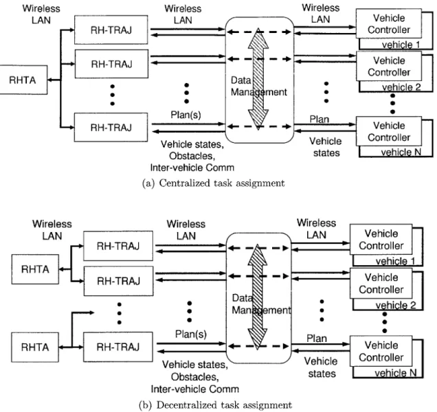
The system infrastructure was setup to emulate a fully integrated fleet of UAVs, but maintain as much simplicity as possible in the vehicles themselves. All data passes through a central hub that performs data management between the planning computers and vehicles, simulating the communication delays, vehicle sensors and uncertainty in the environment. Using this approach greatly simplifies the setup of

Wireless LAN RHTA + Vehicle states, Obstacles, Inter-vehicle Comm

(b) Decentralized task assignment

Figure 1-2: Testbed infrastructure showing ability to evaluate different ar-chitectures for task assignment.

the testbed, while maintaining nearly all of the functionality of a fully integrated system. For example, as shown in Figures 1-2(a) and 1-2(b), the testbed can be used to investigate the impact of communication networking issues on the coordination problem by imposing various limitations and constraints on how the planning laptops communicate (using their own wireless or Ethernet links). The testbed will be used to demonstrate the effectiveness of various control architectures on the task assignment process, as would be seen in utilizing dynamic sub-teams of various compositions.

A key feature of the setup of this testbed is that much of the complexity of the

system has been kept off-board the vehicles. This allows the aircraft to be scaled

LAN RH-TRAJ 4A- - -- RH-TRAJ Data eMan, ament Plan(s) RH-TRAJ Vehicle states, Obstacles, Inter-vehicle Comm

Figure 1-3: The fleet of 8 identical trainer ARF 60 aircraft used in the

multi-UAV testbed at MIT.

smaller than would be necessary if additional computers, batteries and other sensors were on board, yet the performance is similar because waypoint plans and high level control commands can be uplinked to the vehicles at a rate of up to 1 HZ. Under the presumption that the low-level vehicle controllers are working well, the planning system would not need to respond faster, and in practice transmissions are made less frequently.

1.2.1

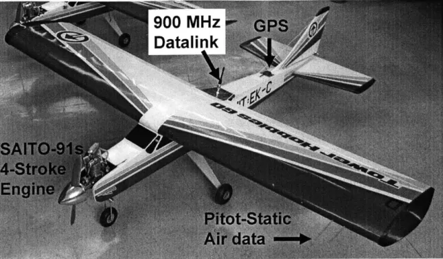
Tower Trainer ARF 60 Aircraft

In order to make successful demonstrations of multi-vehicle flights, the logistics require that the vehicles all have adequate minimum flight durations to ensure that there is sufficient time to perform the required ground operations. For a fleet of four vehicles, flight times greater than 40 minutes are needed in order to have sufficient time in the air to perform experiments. In addition, the vehicles must have sufficient wing loading capacity to carry additional weight from sensors and batteries. The vehicles selected for the testbed are commercially available Tower Trainer ARF 60 aircraft, which have easy handling characteristics and relatively large payload capacities. Only minor modifications are required to augment this class of aircraft to suit the mission requirements, which means that they can be quickly constructed and standardized across the entire fleet. In addition, maintenance and repairs are made much simpler

by utilizing cheap, standardized aircraft for the fleet, and the logistics of flight tests

Figure 1-4: The trainer ARF 60 aircraft used in the multi-UAV testbed at

MIT.

fleet of 8 trainer ARF aircraft are shown together in Figure 1-3.

The ARF 60 aircraft is shown in Figure 1-4, with a table of important aircraft parameters in Table 1.1. The large wing area of the aircraft, combined with the four-stroke, Saito-91s (91 ccs) engine provides more than 3 lbs. of payload capacity, which is sufficient for the avionics, batteries, and additional sensors. An external fuel tank more than doubles the fuel capacity of the aircraft, which allows for extended flights of greater than 50 minutes with moderate throttle settings. The integration of GPS and air data sensors are minor modifications, providing the necessary measurements for autopilot control.

The tower trainer aircraft are well suited for autopilot control because of their stable design for pilot training purposes. The stable configuration causes them to be less susceptible to upsets caused by turbulence, and the aircraft trim states are easily determined. However because the aircraft is so stable, maneuverability is sacrificed. The reduction in performance, combined with minimum flight speeds of ~20 m/s, dictate that slightly larger test areas be utilized to perform effective demonstrations,

(a) (b)

Figure 1-5: Overhead video of the local flying field at Crow Island in May-nard, MA taken with the onboard video system.

Table 1.1: Trainer 60 ARF aircraft parameters

however this tradeoff makes sense for the proof-of-concept missions attempted in this phase of the project.

Additional video and magnetometer sensors have also been integrated onboard the aircraft to provide added real-time measurements about the environment. The pan/tilt video camera (shown in Figure 1-5(a)) transmits video over the 2.4GHz band to the ground-station where it can be processed to track ground objects. Figure 1-5(b) shows a captured image from the video system in flight. The onboard magnetometer provides true heading estimates of the aircraft in flight, which can also be used to provide estimates of the ambient winds acting on the vehicle.

Measurement Value Units

(SI)

Wing Span 1.707 m

Wing Area 0.5200 m2

Chord Length 0.305 m

Wing Incidence 1 deg

Wing Dihedral 5 deg

Gross Mass 5.267 kg

1.2.2 Autopilot

At the time the aircraft testbed was designed, the options for low-level vehicle control included either purchasing or constructing low-level autopilots. Due to proprietary source code restrictions, purchasing an autopilot would be less flexible to suit the re-quirements of the planning system, however the tradeoff in the time to complete the same tasks were significant1. As a result, the decision to purchase the equipment was

made. After considering various options, the decision was made to use the PiccoloTM autopilot from Cloud Cap Technology (Figure 1-6(a)). This autopilot is used onboard the aircraft to perform the autonomous vehicle stabilization and waypoint navigation. One watt transmission of data over the 912 MHz datalink permits the vehicles to nav-igate up to three miles from the ground station (Figure 1-6(b)) and this link can also be used to continuously upload new flight plans and other control commands from ground based planning algorithms. Real-time aircraft telemetry is utilized in ground based processing, including GPS position and velocity (±2m, ±0. 1m/s respectively) air data, attitude estimates, static wind estimates and other control data. The atti-tude solutions are real time estimates obtained using measurements from Cloud Cap's Crista IMU, which provide high bandwidth, angle-rates and accelerations (±3000/s at 16 bits and ±l0g at 16 bits respectively). This information is obtained at a rate of 1 HZ through the robust 912 MHz link providing sufficient bandwidth for high level commands.

Benefits of purchasing a commercially available system are the significant time and effort saved in developing the required infrastructure to tune and test the system. The well-designed and user-configurable Cloud Cap architecture comes complete with a high fidelity hardware-in-the-loop (HWIL) simulation mode that enables real-time testing of the system on the ground before flight tests are performed. While this is primarily meant to simulate the system for controller tuning purposes, it is also interfaced with the planning system so that multi-vehicle simulations can be executed with high levels of accuracy on the ground.

'Similar projects at MIT had taken 4 years to develop their own autopilot. Recent projects at Stanford University have taken similar periods of time.

(a) Commercially available PiccoloTMAutopilot (b) Cloud Cap groundstation with 912 MHz

ra-from Cloud Cap Technologies. dio antenna and Pilot Console.

Figure 1-6: The commercially available Cloud Cap autopilot system.

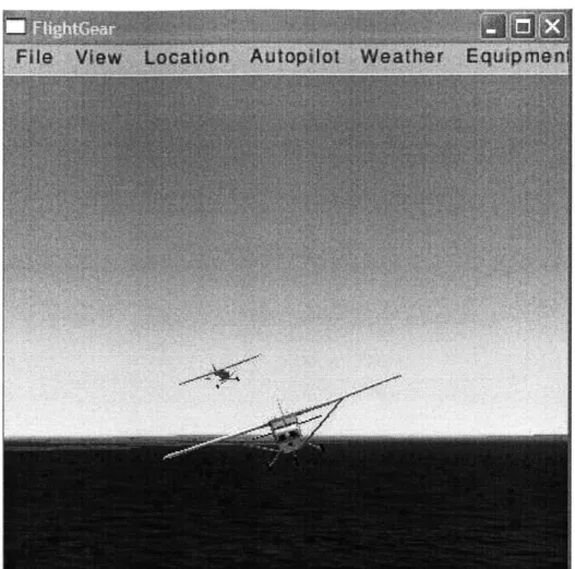
Figure 1-7 displays the setup of the system with the avionics performing HWIL simulations and the planning system in the loop. The groundstation communicates with each of the avionics through the 912 MHz data link, and the telemetry data from the vehicles is passed on to the planning system through integrated TCP/IP protocols, exactly as would be performed during an actual flight test. An integrated GUI is connected to the system to allow user feedback to the planning system and visualize the state of the mission in real-time as shown in Figure 1-8, using FlightGearVO.9.2 operated in network connection mode.

While performing HWIL simulations, each of the avionics is connected through a USB-CAN adapter to a simulator CPU which stimulates the avionics sensors with simulated measurements. The HWIL simulator application allows the specification of a detailed aircraft model that is built up from aircraft geometry and inertia measure-ments or alternatively specified through calibrated wind tunnel data. By specifying the appropriate aircraft parameters and selecting suitable models for sensors onboard, actuator delays and turbulence parameters, an accurate simulation of flying charac-teristics can be built up. This is an essential part of the process in validating control settings and testing the performance of the system before attempting an actual flight. In Chapter 2, the HWIL simulation environment is described in more detail and the flight parameters for the ARF 60 aircraft are explicitly determined.

Hardware-in-the ----

Ainc--Events 10 Loop Simulation

CPUs

--- -- --- -- -- -- --- -- -- -- -- -- -- --G roundstation

Trajectory Plan Cloud Cap 900 Mhz

r Datalink

Optimizatio Processor Interface D

; Cloud Cap

~---Mission PlanTrnmte

Ste Dcisions

Operato

Figure 1-7: Hardware-in-the-loop configuration for the UAV testbed allowing simultaneous simulation of 8 aircraft with the integrated plan-ning system connected through the 912 MHz data link, exactly as would be performed in flight.

1.3

Thesis Outline

Chapter 2 uses identification and analytical methods to find approximate models for the ARF 60 aircraft and verifies that the hardware-in-the-loop simulator reproduces motion consistent with these models. The Cloud Cap autopilot is tuned for the testbed aircraft and closed loop responses are determined to provide more accurate models to be used on the planning level. Chapter 3 introduces the notion of distur-bance estimation into the planning level and accounts for uncertainty in the bounded errors in these estimates. Part of the strategy for rejecting these disturbance estima-tion errors includes implementing timing control to vary the reference speed of the aircraft to reject relative timing errors on the vehicle level. Chapter 4 implements

Figure 1-8: FlightgearVO.9.2 visualization support for the HWIL simulation

environment.

position and heading feedback on the planning level to account for difference between the planned MILP trajectory and the one that is actually flown by the aircraft. This includes dealing with the effect of initial condition uncertainty due to measurement errors and computation delay, as well as the required reductions in authority on the planning level.

Chapter 2

Hardware In the Loop Modeling

and Simulation

The hardware-in-the-loop (HWIL) simulation is only useful if it accurately portrays the vehicle dynamics and if the behaviors observed during flight tests can be repli-cated on the ground. This chapter focuses on identifying some of the dynamical modes of flight for the 60 ARF Trainer aircraft, and verifying that the HWIL sim-ulations reflect the dynamics expected from the aircraft being employed. Reduced order models for 4 of the 5 dynamical modes are determined for the trainer ARF

60 aircraft using identification techniques on experimental flight data and analytical

predictions based on aircraft geometry and aerodynamic data. Section 2.1 describes the simulation settings used to create the hardware-in-the-loop (HWIL) simulations, and Section 2.2 details the procedures used to create models of the aircraft dynam-ics from data collected during flight tests and hardware-in-the-loop simulations. In Section 2.3, the Cloud Cap autopilot is tuned for the trainer ARF 60 aircraft and the closed loop response for several of the modes is measured using the HWIL simulator.

2.1

Hardware in the loop simulations

2.1.1

Aircraft simulation Model Parameters

Aerodynamic, inertial and engine calibration information is provided to the Cloud Cap HWIL simulation application to model the aircraft being flown. For simply

a)

hh rd

(a) The Clark YII airfoil geometry.

(b) The Clark

a [deg]

YH airfoil lift and drag curves.

The Clark YH airfoil closely resembles the airfoil used on the trainer ARF 60 aircraft and is used to model wing aerodynamics. configured aircraft such as the tower trainer 60 ARF used in the testbed, many of the performance characteristics can be obtained using the geometry of the aircraft, such as the data found in Table 2.1. Detailed descriptions of the surface geometry, wing lift curves, and engine performance curves enable simulations of the aircraft under realistic flight conditions, providing the input parameters are configured accurately. For example, the Clark YH airfoil closely resembles the trainer ARF 60 airfoil and is used to describe the aerodynamic properties of the main wing on the aircraft

[25].

Some of the data is shown in Figure 2-1. A more detailed description of the simulator input files is given in Ref. [26].

Table 2.1: Trainer 60 ARF measurements, experimentally determined iner-tias as shown in Subsection 2.1.1. Symbolic notation is borrowed from Ref. [27]

Aircraft Inertia Experiment

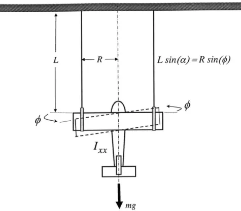
The aircraft pitch, roll, and yaw inertias are important parameters for the accurate HWIL simulation of the aircraft dynamics. Fortunately, due to the small scale of the aircraft, experimental measurements can be easily made for each axis of the aircraft. The experimental setup for the roll axis is shown in Figure 2-2. From the aircraft free body diagram, the tension in each cable, T, is

(2.1) 2T = mg

Measurement Value Units Symbol

(SI)

Wing Span 1.707 m b

Wing Area 0.5200 m2

S

Chord Length 0.305 m

Wing Incidence 1 deg

Wing Dihedral 5 deg I'

Wing Sweep 0.0 deg A

Tail Area 0.0879 m2 _St

Tail Span 0.606 m be

Tail Offset X 1.14 m it

Tail Sweep 9 deg At

Fin Area 0.0324 m2 _Sf

Fin Span 0.216 m bf

Fin Offset X 1.143 m if

Fin Offset Z 0.120 m hf

Fin Sweep 53 deg Af

Fin Volume Ratio 0.0189 - Vf

Fuselage CX Area 0.130 m2 Sb Fuselage Length 1.270 m lb Gross Mass 5.267 kg m Empty Mass 4.798 kg me Roll Inertia* 0.31 kg -m2 Pitch Inertia* 0.46 kg. m2 Yaw Inertia* 0.63 kg -m2

L sin(a) =R sin(#)

mg

Figure 2-2: Torsional pendulum experimental setup to determine roll axis

inertia, I,, for the trainer aircraft. The period of oscillation of a roll angle perturbation,

#,

is measured to parameterize the aircraft inertia. The angle a is the small angle deviation of the supporting cables from the vertical position. This experiment was also repeated for the pitch and yaw axes to determine I, and Izz respectively.

For rotational perturbations applied to the airframe, the product of interior angles and distances must be constant

R# = La (2.2)

where

#

is the aircraft roll angle perturbation and a is the small angle deviation of the supporting cables from the vertical position. The differential equation describing the motion of the torsional pendulum is governed by a torsional inertia term and the restoring moment due to tension forces

I22< + 2TR sin a = 0 (2.3)

Table 2.2: Experimentally determined aircraft inertias [kg-m2_]

Aircraft Roll Axis Pitch Axis Yaw Axis

No. IXX IVV Izz

1 0.28 0.46 0.65

2 0.30 0.44 0.61

3 0.33 0.47 0.63

Mean 0.30 0.42 0.63

Std Dev. 0.029 0.011 0.021

Using the small angle approximation for a since L

>

R, and substituting known values from Eqs. 2.1 and 2.2, Eq. 2.3 reduces to

mgR2

ILzO+ _L $=0 (2.4)

which is characterized by the undamped natural frequency, w, and period of

oscilla-tion, T,

mg R2 (2.5)

IxxL 27ir Ty = 2(2.6)

By finding averaged values for the period of oscillation, T,, in each of the pitch, roll,

and yaw axes, the inertia about each axis can be approximated. This experiment neglects aerodynamic and other forms of damping as well as the cross-axis inertias (e.g., Iz, lyz). The experimental results are summarized for each of the axes and three

different aircraft in the same configuration in Table 2.2, showing agreement between different vehicles used in the tests. The largest variation was found in the roll axis due to the difficulty of mounting the aircraft through the center of gravity, which is essential in this experimental setup.

2.1.2

Actuator Models

The servos used on the aircraft have saturation limits, limited bandwidth, and limited slew rates which are captured in the actuation models of the Cloud Cap

hardware-Actutor I22zwn+n2

Input Input

Saturation Scaling Actuator Transfer Fcn

Figure 2-3: Actuator models used the Cloud Cap

ulations in-the-loop

is given by

W-0

PPActu~

Output Output O

Saturation Rate Limiter

Hardware-in-the-loop

sim-simulator. As shown in Ref. [26], the actuator transfer function, Gaet(s),

specifying the bandwidth limit, Bw

2

Gact(s) = 2+2 _(2.7)

n= 27rBw (2.8)

= (c = 0.707 (2.9)

where the damping ratio,

C,

is selected at the critical value to set the actuator band-width equal to the natural frequency (wb = Wn) . The aileron, elevator, and rudder channels all respond with approximately the same characteristics (Bw = 10 Hz), but

the throttle is modeled with less dynamic range (Bw = 2 Hz) as the engine RPM requires added time to ramp up to produce thrust. The input/output saturation and slew rate limits are determined as per manufacturer specifications (±600, 2 Hz respectively), and applied as shown in Figure 2-3.

2.1.3

Sensor Noises

The Cloud Cap hardware-in-the-loop simulator includes detailed sensor models based on information from the manufacturer to corrupt the simulation measurements. For the purposes of simulation, noises on the pressure, rate gyros and accelerometers onboard the aircraft are modeled using band-limited white noise and specified drift rates [26]. Although the same noise and drift models could be applied to GPS position and velocity measurements, this information is typically assumed to be perfect in the HWIL tests. The values used to parameterize the PiccoloTM pressure sensors, the CristaTM IMU angle-rate sensors, and the accelerometers are shown in Table 2.3.

itr ut

Table 2.3: Crista IMU HWIL Sensor Noise Models

2.1.4

Dryden Turbulence

Stochastic turbulence disturbances are required for accurate HWIL simulations, as real world experiments are characterized by unpredictable winds acting on the vehicle. The Dryden turbulence model is one of the accepted methods for including turbulence in aircraft simulations [28]. By applying shaped noise with known spectral properties as velocity and angle rate perturbations to the body axes of the vehicle, the effect of turbulence is captured during discrete time simulations. The noise spectrum for each of the perturbations is predominantly described by a turbulence scale length parameter, L, the airspeed reference velocity, V, and the turbulence intensity, o-. The selection of these parameters allows for the turbulence to be modeled according to the prevailing wind conditions.

The spectral frequency content for generalized aircraft turbulence have been well studied [29, 28] and are given for each of the aircraft body axes:

2uo2Lu 1 Sug(w) W)2

(2.10)

o2 1+3( Lo )2 Svg (w) = oII 2 (2.11) rVo I + (LW)2) 2Lw 1+3( o)2 S.9(w) = V. 2 (2.12) 'grVo _{1 +} ( Iw)2)

Sensor PDynamic PStatic Gyro Accel.

[unit] [Pa] [Pa] [deg/s] [m/s/s]

Resolution [unit] 3.906 2.00 1.6E-4 6.0E-3

Min [unit] -300 0.0 -5.20 -100.0

Max [unit] 4000 110,000 5.20 100.0

Noise Gain 20.0 20.0 0.10 0.0

Butterworth Order 2 2 2 2

BW Cutoff Freq. [Hz] 11.0 11.0 20.0 20.0

Drift Rate [unit/s] 0.05 1.0 1.5E-4 2.OE-3

Max Drift value [unit] 15.0 100.0 0.01 0.20

S 2 0.8 (rL) )1/3( S,,w)- 4b (2.13) LwVo +(4 O LO )2VIWI Sqg (w) = v -2 Swg(w) (2.14) 1 +

(

4bw) 7rY0

specral frqunc ofg th(()W2

)

(2.15)

where w is the spectral frequency of the turbulence and the aircraft wingspan, b, is used as a parameter in the angle rate filters to scale the effect of rotation on the main lifting surface. The subscripts u, v, w and p, q, r refer to the familiar body frame aircraft wind velocities and angle rates, respectively, thereby allowing independent classification of the turbulence in each axis. These spectral shaping functions are used to form shaping filters to give the body axis noise transfer functions [30]

L1 Hug (s) =a, 2 * L (2.16) rV0 1

+

_V. L 1V+V35Ls Hg (s) = Uo L ( + V.)2 (2.17) L 1+ v/53-L s Hwg(s) = Yw) L + 2 (2.18) rao irV.1+ LS VLO 8 7r 1/6 Hpg(s) = 0m 0. 4b (2.19) L 1/3 ₊₍₄ ) Hqg(s) = Hwg (s) (2.20) 1+ ( b) S Hrg(s) = voI Hvg (s) (2.21) 1+

(

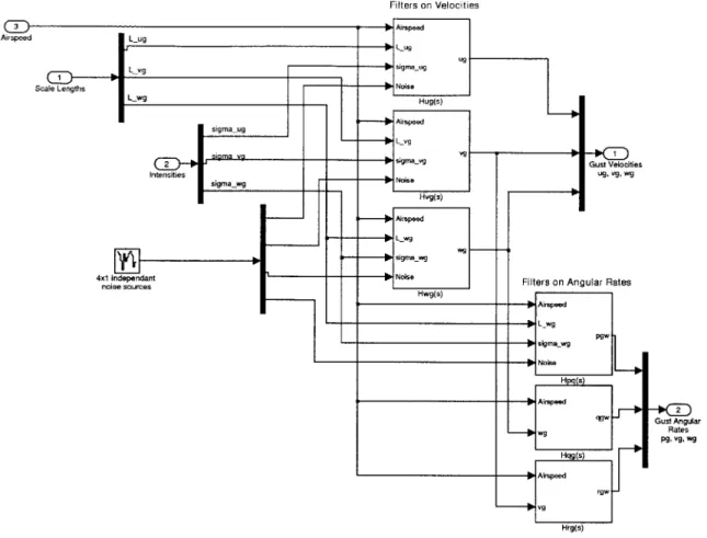
_7rV3b 0Y)

The block diagram for the full 6 DOF Dryden turbulence model is shown in Figure 2-4. Note the cross axis couplings of the angle rate filters qy and rg.

Example turbulence perturbations values are plotted in Figure 2-5 as a function of the scale lengths and intensities for each of the body axes. The same 4 x 1 white noise input was used for each trial set. Larger scale lengths, L, increase the time constant of

Filters on Velocities Airspeed Scale Lengths Gust Velocibes ug. Vg. W9 pg, vg, wg

Figure 2-4: Block diagram for the 6 DOF Dryden Turbulence model. The velocity perturbations ug, Vg, Wg are independent outputs of the

filtered values of the turbulence scale lengths, L, intensity values, o and the white noise input sources. The principle axis coupling of the aircraft is taken into account through the inputs to the angle rate perturbation filters.

the turbulence seen for a given airspeed, while larger o- values increase the deviation about zero. L and o typically vary with altitude in the lower atmosphere as ground effects become more prominent, but for HWIL simulations they are usually fixed.

The frequency response of the Dryden filters are shown for the same three cases in Figure 2-6. The filter cutoff frequency is determined by the ratio of the scale length to airspeed, and this effectively produces lower bandwidth filters for larger scale lengths. The scale length parameter is chosen according to one of several specifications, all of which take into account the variation of L with altitude. The military reference

0.5 5 0 -0.5 > 0 -1 0 1 2 3 4 5 6 7 8 9 -iS 0 1 2 3 4 5 6 7 8 9 Time [s]

(a) Velocity perturbations

0 1 2 3 4 5 6 7 8 9 -0.2 0

0

1 2 3 4 5 6 7 8 9 -0.1 -0.2-0 1 2 3 4 5 6 7 8 9 Time [s]

(b) Angle rate perturbations

Figure 2-5: The output of the Dryden velocity and angle rate filters for

different selections of the intensity and scale lengths. Set 1:

L 150,o = 0.5, Set 2: L = 1500, o- = 0.5, Set 3: L = 150, o-= 1.5 0.

0

0.2 0 0

-is valid up to 1000 feet [29].

LW = h (2.22)

h

LU = LV = ( 2.23)

(0.177 + 0.000823h)1 2

The turbulence intensity is a gain factor that scales the magnitude plots in Fig-ure 2-6 to values appropriate for different wind levels (i.e., light, moderate, severe). The intensity level has been defined for low altitude flight according to MIL-F-8785C

as

o- = 0.1W2 0 (2.24)

o-, = o-, = U" (2.25)

(0.177 + 0.000823h)0-4

where W20 is the wind speed as measured at 20 ft in altitude. According to

MIL-F-8785C, W20 < 15 knots is classified as "light" turbulence, W2 0 ~ 30 knots is "moderate", and W20 > 45 knots is "heavy". Other military specifications such as

MIL-HDBK-1797 exist for the low altitude cases [29], and different types of models

are used for other regions of the atmosphere. For the purposes of the UAV application, the low altitude models are sufficient.

The utility of the Dryden turbulence model is that it allows the expected turbu-lence levels to be described for an aircraft flying at a given reference speed for more realistic HWIL simulations. Turbulence is applied to the vehicle body axes consistent with the known parameterized values for scale length and intensity, which effectively defines the appropriate filters with cutoff frequencies and magnitudes needed for sim-ulation. Note that in addition to turbulence, wind is also usually modeled with a static component, W, that represents a prevailing magnitude and direction in an inertial axis. Together these define an arbitrary three-axis wind vector

W =W + 6W' (2.26)

where SW' is the effective Dryden wind turbulence in each axis after being rotated through the appropriate body to inertial transformation direction cosine matrix.

For small scale aircraft, the static wind component is usually a gross disturbance relative to the aircraft airspeed, and it can have a large effect on high level planning

Bode Diagram

10 10 10 10 10

Frequency (rad/sec)

(a) Velocity filter for w_

Bode Diagram

0 f .... .... ... .. .. ... ..-

---10

10 10 10' 10 10 10 0

Frequency (rad/sec)

(b) Angle rate filter for qg

Figure 2-6: The Bode plots of the Dryden velocity and angle rate filters, given white noise inputs to Ho9(s) in (a) and Hqg(s) - Heg(s)

in (b). Various selections of the intensity and scale lengths are

shown in different sets. Set 1: L = 150,o- = 0.5, Set 2: L = 1500,

algorithms. The effect of this type of disturbance on the planning system and aircraft dynamics is discussed in more detail in Chapters 4 and 5.

2.2

Open Loop Aircraft Modeling

2.2.1

Longitudinal Dynamics

A common model for the longitudinal motion of the aircraft is [27, 311

1 zu XU zw Xq X U X

WU Z' Zq Ze W + r e (2.27)

mU mW mq me q m6,

L 0 0 1 0 0 0

+ = Ax+Bu (2.28)

where the state variables x = [u w q 0]T refer to the longitudinal velocities, u and

w, the pitch rate, q and the angle of inclination, 0. The elements of the A matrix

in Eq. 2.27 represent the concise form aerodynamic stability derivatives referring to the airplane body axis. Tables of values relating the concise form derivatives to the dimensionless or dimensional derivatives are available in numerous sources [27, 32]. The control input u = 6e is the elevator defection angle with the engine thrust fixed

and is input to the dynamics through the aerodynamic control derivative matrix B. The Longitudinal Dynamics in Eq. 2.27 are typically resolved into two distinct phugoid and short period modes, which represent dynamics of the aircraft on different timescales. The short period is characterized by high frequency pitch rate oscillations and can have high or low damping, depending on the dynamic stability of the aircraft. In contrast, the phugoid mode is characterized by lightly damped, low frequency oscillations in altitude and airspeed with pitch angle rates, q, remaining small.

Short Period Mode

A simple approximation for the short period mode of the aircraft can be obtained by

assuming the speed of the aircraft is constant over the timescale of the short period dynamics (t = 0), that the aircraft is initially in steady level flight and that the

derivatives refer to a wind-axis system (0 = 0). The equations of motion then

reduce to

[1Z

Zq

iFW

1+

_{6e c (2.29)}

[q mW mq q m ,

Following further approximations shown in [27] which make assumptions about the relative size of the mq, Zq and zw derivatives, the transfer functions for the two short term equations describing the response to elevator are:

w(s) z2__ s_+_VoA _{k(s + 1/T) (2.30)}

6e(s) (s2 - (mq + zw)s + (mqzw - mwVo)) s2 + 2C8wes +w2

q(s) _ mn(s - zW) A kq(s + 1/To) (2.31)

6e(S) (s2 - (mq + zW)s + (mqzw - mWV₀)) s2 + 2(8was +w2

where kq, kw, To, T, (,, and w, represent approximate values for the short period mode and V is the vehicle reference speed.

One of the most accurate ways to obtain models for the aircraft data is to use actual flight data. Identification algorithms such as those in the Matlab System Iden-tification Toolbox [33] can be used to used to obtain open loop models of the system dynamics from flight data collected during experiments. These models can then be used to validate the HWIL simulation environment as well as to help determine the gain settings for the autopilot control loops as shown in Section 2.3. Input-output data was collected by disengaging all of the autopilot loops and performing a series of maneuvers to measure the aircraft response to deflections from the elevator and aileron control surfaces. Example data from two experiments are shown in Figures 2-7(a)-(b) depicting the longitudinal and lateral modes, respectively.

To capture the longitudinal dynamics, the bank angle was held fixed at zero degrees, while a series of pitch oscillations were commanded using the elevator. Figure 2-7(a) shows a sample of data that was collected on one run of the pitch test. From the plot it is clear that the longitudinal modes are being excited due to input from the elevator, while the lateral motions in the roll and yaw axes are essentially fixed. Sample data from a roll excitation run is plotted in Figure 2-7(b). This plot also clearly shows coupling in the yaw axis due to the dihedral angle of the wing.

U) CO-0 ~U) - C (L-a 100 50-0 -50--100 40 20 - 0- -20--40 0- 100100 -0 100 -1055 100 50 - 0--50 --100 - I - -, - -4 -,%1A" I -- ~.i ~.1 ~j 308 310 312 Time [s] 314

(b) Roll test data induced with aileron deflections. Note the yaw axis coupling due

to the large dihedral angle of the wing

Figure 2-7: Sample flight test data used in the estimation algorithms.

Dash-dot lines represent rate gyro data output for each axis. Control surface inputs are plotted for each corresponding axis in degrees of deflection 'j~;; '~i* cc 0) a) A ~~I 1 t 50 x U) 0-as -- 50 100-'- ' 1080 1085 - I '.'- '-_'4, -' ~,4, I 'I U. (0 U) zU 10 ~0 10 -306 316 318 -r -- Aile -- Rudd 0 --- Elev 1060 1065 1070 1075 time [s] -- , 1b ! %;

Parametric models for the input-output transfer functions can be formed using experimentally collected data and used to determine the unknown coefficients in

Eq. 2.31. Then from the characteristic equation, the longitudinal short period

dy-namics can be inferred from models of the transfer function from elevator angle to pitch rate. Also note that qualitative predictions about the values of the parameters in Eq. 2.31 are available, since they depend on the concise stability derivatives which all have physical significance. Once models are obtained the approximate parameters can then be verified against these qualitative predictions.

Figure 2-8 shows the output of a parametric subspace model based on experimental data such as that shown in Figure 2-7(a). The model output (solid line) tracks the actual measurements of pitch rate (dashed line) quite well and was validated on data sets from different test days and aircraft. Model residuals within the 99% confidence bounds for the auto- and cross correlation functions are plotted in Figure 2-9 and indicate that the 3rd order model is sufficient to describe the input-output dynamics.

This model is represented by the continuous transfer function in Eq. 2.32 and has zero-pole pairs as indicated in Figure 2-10(a). The short period is well represented by the high frequency, oscillatory mode of the system, while there is one low frequency pole located near the imaginary axis. The transfer function is:

q(s) 9.539s2 - 1440s + 60.52

T6 = 6e(S) S3 + 21.77s2 + 325.8s + 29.94

9.539(s - 150.9)(s - 0.0420) (s2 _{+ 21.7s + 323.7) (s + 0.0925)}

The third order model Tqe,(s) was selected because it provided the best fits to a large number of data sets and residuals that remained below the 99% confidence intervals in Figure 2-9. Approximate values for the short period dynamics can be obtained by resolving the oscillatory mode in Eq. 2.32 to determine the corresponding values for w, and (. A step response for this mode is plotted in Figure 2-10(b),

indicating a reasonable short period response time with settling time 0.4 seconds, and

(, = 0.6. Second order models produced from the same data set were found to have

difficulty reproducing the outputs of the experiment, and exceeded the confidence bounds as shown in Figure 2-9. Higher order models (4th and higher) tended to