Development of energy efficient membrane distillation systems

Development of Energy Efficient Membrane

Distillation Systems

by

Edward K. Summers

S.M., Massachusetts Institute of Technology (2010)

S.B., Massachusetts Institute of Technology (2008)

Submitted to the Department of Mechanical Engineerin

in partial fulfillment of the requirements for the degree of

Doctor of Philosophy

at the

MASSACHUSETTS INSTITUTE OF TECHNOLOGY

June 2013

@

Massachusetts Institute of Technology 2013. All rights reserved.

Author...

?.

Department of Mechanical Engineering

May 16, 2013

Certified by...

...

John H. Lienhard V

'olins Pro ssor of Mechanical Engineering

Thesis Supervisor

A ccepted by ...

...

David E. Hardt

Graduate Officer, Department of Mechanical Engineering

ARCHNIFS

OF TECHN0LOGY

JUN 2

2013

Development of Energy Efficient Membrane Distillation

Systems

by

Edward K. Summers

Submitted to the Department of Mechanical Engineering on May 16, 2013, in partial fulfillment of the

requirements for the degree of Doctor of Philosophy

Abstract

Membrane distillation (MD) has shown potential as a means of desalination and water purification. As a thermally driven membrane technology which runs at relatively low pressure, which can withstand high salinity feed streams, and which is potentially more resistant to fouling, MD could be used for desalination where reverse osmosis is inadequate. The use of thermal energy, and the ease of construction at small scale, makes this technology attractive for off-grid or renewable power applications as well. However, most research on MD has focused on maximizing purified water output per unit of membrane area as opposed to minimizing system energy consumption and cost. Current MD systems suffer from poor energy efficiency, with reported performance rarely exceeding that of a simple solar still.

This thesis explores means to optimize the design of MD for energy efficiency to make it competitive with existing thermal desalination systems, with particular focus on the Air Gap Membrane Distillation (AGMD) configuration. A detailed

ID numerical model to explore the effect of design parameters on energy efficiency

was developed. Means to enhance energy recovery from hot discharge brine without additional brine concentration, and reduce diffusion resistance by means of reducing pressure in the air gap were explored. A novel configuration delivering solar flux directly to the membrane, and multi-stage, multi-pressure configurations comparable to MSF were also developed. A parameter to relate the performance of a bench-scale experiment with similar membrane and gap size to a production system was developed and validated.

Small scale experiments were conducted to verify performance for the novel solar powered configuration, reduced gap pressure, and capturing energy from hot dis-charge brine. Experiments demonstrated the efficacy of a solar absorbing membrane to provide heat to the cycle, and established a benefit of deforming the membrane

into the gap under hydraulic pressure; reducing gap size and measurably improving performance. Parametric studies have shown the effectiveness of using the model to design larger, more practical, competitive systems; establishing the importance of long flow lengths, low mean membrane flux, and large membrane area in the design of efficient MD systems.

Thesis Supervisor: John H. Lienhard V

Acknowledgments

Thank you to my advisor, Prof. John Lienhard V, for his guidance, and to my labmates, who were always willing to discuss ideas and offer advice.

Thank you to my thesis committee, Prof. Alexander Mitsos, Prof. Gregory Rut-ledge, and Prof. Hassan Arafat, for providing valuable feedback over the course of my research.

Also, to the Masdar Institute for funding this project and assuring I got a pay-check.

Thank you to our co-collabrators at Masdar, Prof. Hassan A. Arafat, Rasha Saffarini, Elena Guillen, and Mohamed Ali for contributing to this work in various respects.

And lastly to my friends and family for their patience and support throughout my time here at MIT.

Contents

1 Introduction

1.1 Membrane Distillation ...

1.1.1 Characteristics of MD . . . . 1.1.2 Previous Work . . . . 1.2 AGMD: Advantages and Potential for Im

2 Analytical Models of MD

2.1 Introduction . . . . 2.2 Common Model Elements . . . .

2.3 Direct Contact MD . . . . 2.4 Air Gap MD . . . .

2.5 Pumped Vacuum MD System . . . . 2.6 Solution Method and Verification . . . .

2.7 Model Validation . . . . 2.7.1 Direct Contact MD . . . .

2.7.2 Air Gap MD . . . .

2.7.3 Pumped Vacuum System . . . . . 2.7.4 Membrane Distillation Coefficient

3 Novel MD Configurations

3.1 Solar Direct Heated Membrane AGMD

3.1.1 M odeling . . . . 3.1.2 Cycle Configurations . . . . provement 21 22 24 25 28 29 29 30 33 35 40 43 43 43 45 46 47 51 51 53 59 Data . . . . . . . . . . . .

3.2 Multi-Stage Vacuum MD . . . . 3.2.1 M odeling . . . .

3.3 Novel Energy Recovery Enhancements . . 3.3.1 Hot Brine Discharge Regeneration .

3.3.2 Reduced Pressure Gap AGMD . . .

4 Experimental Validation

4.1 Experimental Scaling ...

4.2 Design and Construction . . . . 4.2.1 Objectives . . . . 4.2.2 Experimental Design . . . . 4.2.3 Solar Direct Heated Experiment . . . . 4.2.4 Spacer Experimentation . . . . 4.3 R esults . . . . 4.3.1 Validation and Reduced Pressure Gap AGMD 4.3.2 Solar Direct Heated System . . . . 4.3.3 Hot Brine Discharge Regeneration . . . .

5 Applications

5.1 Parametric Study of MD Systems - Optimal Configurations . . . .

5.1.1 Module Geometry . . . .

5.1.2 Operating Conditions: Temperature and Mass Flow Rate . . . 5.1.3 Relationship Between Recovery Ratio and GOR . . . . 5.1.4 Comparison of VMD: Use of Brine Energy Recovery . . . .

5.2 Large-Scale Solar Direct Heated AGMD . . . . 5.2.1 Comparison of GOR Between Different Solar Heating

Configu-rations: A Simple Direct Heated System . . . .

5.2.2 Conclusions . . . .

5.3 MSF-Competitive Multi-Stage VMD System . . . . 5.3.1 Energy Efficiency Comparison . . . .

5.3.2 Irreversibility Comparison - Entropy Generation . . . .

. . . . 6 1 . . . . 6 3 . . . . 6 5 . . . . 6 5 . . . . 6 7 71 . . . . 7 1 . . . . 8 1 . . . . 8 1 . . . . 82 . . . . 86 . . . . 88 . . . . 92 . . . . 92 . . . . 97 . . . . 100 103 103 106 108 111 112 116 118 120 121 122 123

5.3.3 Conclusions . . . .. . . . . 126

6 Conclusions

6.1 M odeling. . . . .

6.2 Experimentation . . . . 6.2.1 Challenges of Small-Scale Experiments

6.3 Future Work . . . . 6.4 Contribution to Collaborative Works . . . . .

127 127 129 130 131 131 . . . . . .. . .- - . . .- . . . . . . . . . . . . . .

List of Figures

1-1 World map detailing physical and economic water scarcity in 2006. . 21

2-1 The feed (hot) side of any MD configuration with heat and mass fluxes

labeled. . . . . 30

2-2 A simple counter flow DCMD module. . . . . 33

2-3 A control volume for a DCMD module cell. . . . . 34

2-4 An AGMD membrane module with an integrated condenser. . . . . . 36

2-5 A control volume of an AGMD module cell. . . . . 36

2-6 A VMD module where permeate is removed by a vacuum pump and condensed... ... 40

2-7 Schematic drawing of a startup curve showing the vacuum pressure and mole fraction of vapor on the permeate side of the module. . . . 41

2-8 Control volume of a VMD membrane module cell. . . . . 42

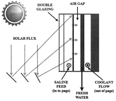
3-1 Schematic diagram of a radiatively heated MD module with energy and m ass flows. . . . . 52

3-2 Side view of a possible solar direct-heated system configuration. . . . 53

3-3 The hot side of the MD membrane receiving heat flux, with heat and m ass fluxes labeled. . . . . 54

3-4 Transmissivity of solar collector glass compared to water in the visible and near infrared spectra . . . . 57

3-5 Loss modes through the solar collecting surface of the module. ... 58

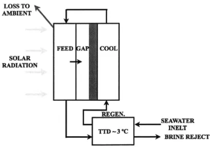
3-7 An AGMD desalination unit with recovery heat exchanger at the

bot-tom of the cycle. . . . . 60

3-8 Temperature profile of the feed side of the membrane for a solar direct heated system and a conventionally heated system. . . . . 61

3-9 Process diagram for a once-through MSF system . . . . 62

3-10 Multi-Stage Vacuum MD (MS-VMD) process diagram. . . . . 63

3-11 Brine regeneration in AGMD . . . . 66

3-12 Comparison of GOR for an AGMD system with and without regener-ation . . . . 67

3-13 Comparison of energy efficiency improvement resulting from reducing the gap size and gap pressure in an AGMD system with 100 m2 _of m embrane area. . . . . 69

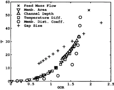
4-1 Non-Dimensional System Parameter T vs. modeled GOR for 66 dif-ferent system s. . . . . 78

4-2 Non-Dimensional System Parameter T vs. GOR with best fit curve . 79 4-3 Relationship of TRR vs. recovery ratio with best fit curve. . . . . 80

4-4 Flow sheet for the experimental setup with all possible configurations show n. . . . . 82

4-5 Serpentine flow channel in a square area. . . . . 83

4-6 Components of MD module "sandwich". . . . . 84

4-7 Assembled module configured to be heated at the top of the cycle. . . 85

4-8 Assembled module with a composite membrane being heated by solar energy. . . . . 87

4-9 Absorptivity of several solar absorbing materials for a composite MD m em brane. . . . . 88

4-10 Open spacer placed over the condenser plate . . . . 89

4-11 Narrow rib spacer, with higher rib frequency. . . . . 90

4-12 Screen spacer with support in both the horizontal and vertical directions. 91 4-13 Two stage water column to reduce gap pressure to as low as 0.4 atm. 92

4-14 Comparison between experimental data and model for a conventionally

heated AGMD system at atmospheric pressure. . . . . 93

4-15 Comparison between experiment and models with and without stretch-ing of the membrane. . . . . 94

4-16 GOR vs. top temperature for various gap pressures. . . . . 95

4-17 GOR vs. top temperature for various gap pressures compared to ex-perimental results at atmospheric pressure. . . . . 95

4-18 GOR vs. top temperature for atmospheric and 0.4 atm gap pressures compared to experiments. . . . . 96

4-19 Recovery ratio vs. top temperature for atmospheric and 0.4 atm gap pressures compared to experiments. . . . . 97

4-20 Flux performance of a solar direct heated system. . . . . 98

4-21 Various heating configurations tested for comparison. . . . . 99

4-22 Comparison of different solar heating configurations . . . . 100

4-23 GOR vs. Heat Input for an conventionally heated system with and without regeneration. . . . . 101

5-1 DCMD system flowsheet. . . . . 104

5-2 AGMD system flowsheet. . . . . 105

5-3 VMD system flowsheets, (A) without and (B) with brine regeneration. 105 5-4 GOR as a function of flow channel height. . . . . 107

5-5 GOR as a function of length in the flow direction. . . . . 107

5-6 GOR as a function of air gap size in an AGMD system. . . . . 108

5-7 GOR as a function of top temperature, Tfin. . . . . 109

5-8 GOR as a function of bottom temperature, Tsw,in . .. . . . . 109

5-9 GOR as a function of mass flow rate. Gaps in lines indicates transition flow region, where heat transfer coefficient is not defined. . . . . 110

5-10 Recovery ratio as a function of length for DCMD and AGMD systems. 112 5-11 GOR as a function of flow channel depth in VMD systems with and without brine regeneration. . . . . 113

5-12 GOR as a function of effective length in the flow direction for VMD

systems with and without brine regeneration. . . . . 114

5-13 GOR as a function of top temperature (T,in) for VMD systems with

and without brine regeneration. . . . . 114 5-14 GOR as a function of bottom temperature (Tswin) for VMD systems

with and without brine regeneration . . . . 115 5-15 GOR as a function of mass flow rate in VMD systems with and without

brine regeneration . . . . 115 5-16 GOR as a function of degree of solar concentration with and without

brine regeneration. . . . . 118 5-17 GOR as a function of feed inlet temperature for two different solar

direct heating configurations and conventional heating. . . . . 120

5-18 GOR as a function of the number of stages in an MS-VMD process. . 123 5-19 Recovery Ratio as a function of the number of stages in an MS-VMD

process. ... ... 124

5-20 Control volumes for comparison of entropy generation between MSF

and M S-VM D. . . . . 125 5-21 Irreversibility comparison between a conventional once-through MSF

List of Tables

1.1 GOR and operating conditions of existing single-stage MD desalination

system s. . . . . 26

2.1 Operating parameters from Martinez-Deiz. . . . . 44

2.2 Comparison between model presented here and an experiment by Martinez-D eiz. . . . . 44

2.3 Operating parameters from Fath et al. . . . . 45

2.4 Comparison between simulation and Fath et al. experiment. . . . . . 46

2.5 Operating parameters from Mericq et al. . . . . 47

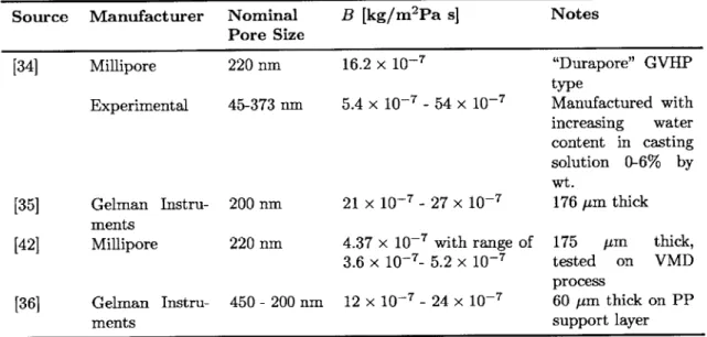
2.6 Experimentally tested membrane distillation coefficients for PTFE mem-branes. Membranes were tested in DCMD configuration unless other-w ise noted. . . . . 49

4.1 Parameters of a baseline AGMD system from which test cases are gen-erated. ... .. . .... .. ... .. .. .. . . . . ... .. .. .. 77

4.2 Experiment attributes and operating parameters. . . . . 86

5.1 Module attributes of a baseline MD module. . . . . 104

5.2 Baseline Properties of a Solar Heated AGMD Module . . . . 116

5.3 Attributes and operating conditions of a simple one-piece solar MD desalination system . . . . . 119

Nomenclature

Roman Symbols

B Membrane distillation coefficient or membrane flux coefficient [kg/m 2Pa s]

c _{Vapor concentration [mol/m} 3_]

co Speed of light [m/s]

C, Specific heat capacity at constant pressure [J/kg K]

dg,,p _{Air gap width [m]}

dA Differential area element [im2

]

dz Differential module length [m] g Acceleration of gravity [m/s2_]

h Enthalpy [J/kg]

ht Convective heat transfer coefficient [W/m 2K]

hfg Latent Heat of Evaporation [J/kg]

h, Planck's constant [J s] I Irradiation [W/m 2_] I, Irradiance [W/m 2 nm] J Vapor flux [kg/m 2_s] k Thermal conductivity [W/m-K] kb Boltzmann's Constant [J/K]

Ket _{Glazing extinction coefficient [1/m]}

fi Mass Flow Rate [kg/s] n Index of refraction

P Total pressure [Pa]

p Partial pressure [Pa]

qIOSS Average heat loss across a membrane module [W/m 2_]

Q

q _{Heat flux [W/m} 2

1

RR Recovery Ratio

r Reflectance

S _{Solar radiation flux absorbed by the membrane [W/m} 2 Sf Solar radiation flux absorbed by the bulk feed stream [W/m 2

TTD Heat exchanger terminal temperature difference [K]

T Temperature [K]

Ut Overall heat loss coefficient [W/m 2_K]

v Specific volume [m 3/kg]

w Membrane width [m]

x Mole Fraction

z Lengthwise Coordinate

Greek Symbols

(Ta) Transmission-absorption product

a Absorptivity

a _{Thermal diffusivity [m}2_/s]

ATf lash Saturation temperature difference between stages [K]

ATht, _{Temperature rise across the heater}

_[C]

ATim Log-mean temperature difference [K]

j Thickness [m]

E Heat exchanger effectiveness A Wavelength [nm]

w Humidity ratio [kg water/kg dry air]

p Density [kg/m 3]

p Reflectivity

0 Beam angle [rad]

r Transmissivity Porosity Subscripts a Air gap abs Absorber air Air b Bulk flow bl Blackbody c Condenser stream c1 Inner cover c2 Outer cover

cond Condenser cooling water

conv Convective heat transfer

exp Isothermal expansion

f

gl Glazing material

i Condensate film interface

in In

I Liquid phase

m Membrane

max Maximum

out Out

I Beam component perpendicular to surface

p Permeate

p, c Condensed permeate in a liquid phase

rad Radiative heat transfer

rej Brine rejected to environment

sat Saturation

stack Glazing stack

SW Seawater

v Vapor

w Water

wall Condenser wall

Chapter 1

Introduction

Currently many areas of the world suffer from a scarcity of fresh water. Despite the fact that the world is over 2/3 water, the vast majority of it is too salty for human consumption. According to the International Water Management Institute [1] many

areas of the world have severe physical water scarcity, as shown in Figure 1-1 [1].

Approwchng physkat water Scrcity

Economic water cartt

Uttie or no water scarnity

Not estimated

Figure 1-1: World map detailing physical and economic water scarcity in 2006 [1].

As the human population grows this problem is only going to be compounded. Desalination can provide a means of expanding the world's supply of fresh water. However, desalination technologies run up against myriad technical and economic challenges. The most common means of desalination, Reverse Osmosis [21 is

gener-ally considered the most efficient, and works by mechanicgener-ally forcing water through salt-impermeable membranes against the osmotic pressure gradient. These systems, however, suffer from high complexity, high capital cost, and a limitation on feed stream salinity where feed streams generally do not exceed 45,000 ppm of dissolved solids [3]. Thermal technologies, popular in the Middle East [2] where thermal energy is more readily available can process a variety of brines, but suffer from fouling and scaling limitations [4].

Therefore, there is a need to develop desalination systems that overcome these barriers, but are also scalable in output and cost efficient, and can be deployed in a variety of areas that do not necessarily have access to large municipal water distri-bution infrastructure or the means to maintain a technically complex system. Tech-nologies that can work in combination with existing desalination processes would also make desalination more accessible to areas suffering from both economic and physical water scarcity.

1.1

Membrane Distillation

Membrane Distillation (MD) is such a technology that could potentially increase the use and accessibility of desalination.

Membrane distillation is a separation process in which a hot feed stream is passed over a microporous hydrophobic membrane. The temperature difference between the two sides of the membrane leads to a vapor pressure difference that causes water to evaporate from the hot side and, pass through the pores to the cold side. The vapor is pure water which can be condensed. This process has application to desalting water. Compared to reverse osmosis, MD does not require a high pressure feed, and can process very high salinity brines. Compared to other large thermal processes, it can be easily scaled down. Demonstrated pilot plants have been used at a small scale (0.1 m3/day), including stand-alone systems disconnected from municipal power or water networks [5, 6, 7].

col-lected from the permeate side. In direct contact MD (DCMD), the vapor is condensed on a pure water stream that contacts the other side of the membrane. In air gap MD

(AGMD), an air gap separates the membrane from a cold condensing plate which

collects vapor that moves across the gap. In sweeping gas MD (SGMD), a carrier gas is used to remove the vapor, which is condensed in a separate component. SGMD is typically used for removing volatile vapors and is typically not used in desalination

[8]. In vacuum MD (VMD), the permeate side is kept at lower pressure to enhance the

pressure difference across the membrane, and condensation may occur in the module, or in an external condenser. All the different configurations of MD can be applied to seawater and brackish water desalination [8, 9]; however, those most commonly used for desalination are DCMD, AGMD, and VMD.

Most research on MD desalination focuses on maximizing membrane flux, or vapor produced per unit area of membrane. However some studies have examined energy efficiency for experimental plants at the 0.1 m3/day scale [5, 6]. Additionally, more recent MD desalination studies have also examined energy efficiency [5, 10, 11, 12]. Using membrane flux as a proxy for thermal performance may not lead to the correct conclusion about overall system performance, as fresh water output and energy con-sumption can be highly dependent on system configuration, membrane area, system top temperature, and heat recovery from hot brine and condensing vapor. In a com-plete cycle, the highest flux may not lead the best use of energy, as it often requires high heat inputs and the resulting high vapor flux can increase resistance to heat and mass transfer, driving up energy use.

Few direct comparisons have been made between the different configurations of MD: DCMD, AGMD, VMD. Studies that have compared different configurations have focused on the processes in the MD module, instead of full thermal cycle per-formance. Cerneaux et al. [13] compared heat and mass transfer processes and total flux over ceramic MD membranes in DCMD, AGMD, and VMD. Alkalibi and Lior compared flux over different MD configurations (including SGMD) [14] and expanded their analysis to include heat and mass transfer characteristics [15]. Ding et al. [16] examined the removal of ammonia from water using MD with a focus on flux and

chemical concentrations. However, no studies have examined MD in the context of a full desalination cycle, where energy recovery is highly important to the viability of a desalination process. Therefore, evaluation of MD in this thesis will be focused on energy efficiency.

1.1.1

Characteristics of MD

DCMD systems in desalination have been studied fairly extensively. While they have

good salt rejection, they suffer high trans-membrane heat loss, and consequently low membrane flux. Typical DCMD systems, tested with NaCl solutions between 35,000 and 100,000 ppm, have achieved a membrane flux from 1-10 L/m 2_{hr [17, 18, 19]. The} biggest disadvantage of these systems is that the cool water on the permeate side results in large conductive heat losses through the thin membrane.

AGMD typically has slightly higher flux for similar temperature conditions, as

the air gap provides thermal insulation between the hot feed and cold condenser water. However, resistance to mass flux is limited by diffusion across the air gap and evaporation through the pores, which is also dependent on the pore size and the resultant trans-membrane diffusion mechanism. Condensate film thickness is typically

10 times thinner than the air gap width [14]. Fluxes for AGMD systems operating

near 70 'C inlet feed temperature range have been reported from 10 L/m 2_{hr [14, 6]} up to 65 L/m 2_{hr [13]. This type of system is most commonly used in pilot-scale} desalination systems [20].

VMD has the best performance in terms of flux as a result of enhancement by the mechanical pressure difference. One system operating at a high temperature of

85 'C [21] achieved a flux of 71 L/m 2_{hr. A second system [13] was able to achieve} a consistent flux of 146 L/m 2hr operating at 300 Pa on the permeate side and with a 40 'C feed inlet temperature. A third system [22] made use of turbulent feed flow and vacuum to enhance flux, achieving 40 L/m2_{hr. The applied vacuum on the} permeate side was roughly half an atmosphere, which can easily be achieved without expensive pumps and pressure vessels. This indicates that a mechanically applied pressure difference is more advantageous when using VMD systems. In cases where

fouling is a concern, mechanical pressure enhancement can keep feed temperatures low while still achieving high flux.

SGMD relies on a sweeping gas to entrain water vapor. It is typically not used in

desalination as the latent heat is not given up into the air stream, and adding moisture to an air stream results in an increase in enthalpy without necessarily increasing the bulk temperature. This makes it hard to recover energy from the permeate stream,

as the moist air sometimes exits close to, or below, the seawater inlet temperature, requiring additional cooling to create the appropriate temperature gradient to transfer heat into the feed stream. The requirement for external cooling has made this cycle too complex and expensive to be realized for desalination, where energy recovery is crucial.

1.1.2

Previous Work

Compared to real-world desalination processes, current MD desalination systems suf-fer from poor energy efficiency. Energy efficiency in this paper will be measured by the gained output ratio, or GOR, defined in Equation 1.1.

GOR = 1h.1

Qin

GOR is the ratio of the latent heat of evaporation of a unit mass of product water to the amount of energy used by a desalination system to produce that unit mass of product. The higher the GOR, the better the performance, as the energy used for evaporation is recovered and recycled multiple times. Amongst thermal systems, a solar still would have a a GOR on the order of 0.5 [23], whereas a good Multi-Effect Distillation system may have a GOR of 12 [24]. Table 1.1 shows the GOR values of existing experimentally tested MD systems with operating conditions when available. GOR is directly proportional the recovery ratio (RR), or the amount fresh water produced per unit feed that enters the system, Equation 1.2 describes the recovery ratio:

RR -f

rnf (1.2)

Considering the heat input, Qj, can be written as the temperature rise of the

feed as it passes through the heater, or ATht, and the capacity rate of the feed, the

GOR can then be written in terms of the recovery ratio and temperature rise required

through the heater:

GOR = RRhfg C, ATht,

(1.3)

In addition to increasing energy recovery in a system, improving GOR also involves improving system recovery ratio by increasing water production or decreasing the amount of feed flow rate required, thereby reducing load on the heater.

Table 1.1: GOR and operating conditions of existing single-stage MD desalination systems. "SP" denotes System Banat et al. (2007) [7] Fath et al. (2008) [6] Guillen-Burrieza et al. (2011) [5] Criscuoli (2008) [25] Wang et al. (2009) [26] Criscuoli (2008) [25] Lee et al. (2011) [11] Zuo et al. (2011) [10] solar powered Type AGMD (SP) AGMD (SP) AGMD (SP) VMD VMD (SP) DCMD DCMD DCMD

systems. Operating conditions listed if given.

GOR Operating Condition

0.9 Clear sky, 40.11 kWh/day absorbed en-ergy, 7 m2 memb. area

0.97 Clear sky, Tt0p = 60-70 *C, 7 m2 area, Tbot = _{40-50 'C, 0.14 kg/sec low rate,}

Seawater

0.8 TtoP= 80 *C+ , 20.1 L/min (0.33 kg/s) feed flow rate, 5.6 m2

memb. area, 2 modules in series, 35,000 PPM feed salinity

0.57 40 cm2 memb. area, 1 kPa permeate pressure

0.85

0.17 40 cm2 _{memb. area}

4.1 0.5 L/min (0.008 kg/sec) feed flow rate,

T = 90 'C, 0.4 m-, 2 memb. area (per

stage), 8 stages in series

1.4 0.04 m/s Feed, 0.48 m/s permeate (hollow fiber, permeate on shell side),

TP=90 'C, 10 m2

area, Tbot= 25 *C, 30,000 PPM feed salinity

Most experimental systems have achieved a GOR of around 1. Larger membrane areas have achieved higher GOR values. With the limited amount of data on VMD systems reported GORs remain rather low, below 1, when compared to tested DCMD and AGMD designs. A wide range of GOR for each type of system shows the depen-dence on configuration and operating conditions. The systems are all at prototype scale, with an output of 0.1-1 m3/day. These results show the need for additional insight on how the design of each type of MD configuration affects the thermal per-formance, which would in turn affect water cost.

Renewable Powered Systems

Solar powered desalination has the potential to provide a solution for arid, water-scarce regions that also benefit from sunny climates, but which are not connected to municipal water and power distribution networks that are necessary for the most common large-scale desalination systems. Solar energy is a natural way provide heat-ing energy or electrical power to a small scale system that must run independent of any other infrastructure.

The most common form of solar desalination is a solar still. Solar stills are simple to build, but inherently do not recycle energy as water condenses on a surface that rejects heat to the ambient environment [23]. Another option of this type is solar powered reverse osmosis. While more energy efficient than any thermal based system, it requires expensive components which are expensive to maintain. RO membranes experience high pressures and can easily be damaged by substances commonly found in seawater, therefore pretreatment is required. As a result, high cost and complexity make these systems unattractive for off-grid or developing world applications.

However, renewable-powered MD systems which have been built currently have poor energy efficiency. When measured by the gained output ratio (GOR) these systems do not exceed the performance of a simple solar still, which typically has a GOR of 0.5-1, as most solar stills do not usually employ energy recovery [27]. Systems with poor energy performance are generally costlier to run, especially if there is a large capital cost associated with solar collection [28]. Table 1.1 lists the

energy performance of existing renewable energy powered MD systems, denoted by "SP",.

1.2

AGMD: Advantages and Potential for

Improve-ment

Of all the systems commonly used for desalination, air gap membrane distillation

(AGMD) shows the strongest potential for improvement. GORs of current AGMD systems tend to be lower than for other systems, and the insulation properties of the air gap prevent direct thermal loss between hot and cold sides. The built in condenser surface allows fluid to be condensed at the local saturation temperature instead of being mixed and condensed at the mean saturation temperature as in a VMD system. Creative design improvements and optimization could potentially make

Chapter 2

Analytical Models of MD

2.1

Introduction

Detailed modeling of the transport processes in an MD module is the first step toward complete cycle modeling, and allows for the identification of performance limiting processes at different operating conditions.

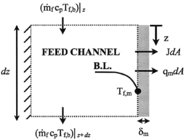
Existing analytical models for MD systems were adapted to be solved numerically (discretized) using a finite difference method. The membrane id divided along its length, L, in the flow direction, into discrete cells of length dz and width w, which multiplied make a differential area element, dA. Bulk flows serve as inputs and outputs for neighboring cells. An example cell of differential length for the feed side of any MD configuration with heat and mass flows illustrated is shown in Figure 2-1. In all cases a counter-flow configuration is used. A large system of equations, describing the heat and mass transfer interactions at each cell are combined with appropriate boundary conditions at the first and last cell and solved using Engineering Equation Solver (EES) [29]. EES is a simultaneous equation solver which uses a Newton iteration method to converge on the solution.

For AGMD, models by Liu et al. [30] and Rattner et al. [31] were used as a basis to solve to heat and mass transfer interactions across the cell. For DCMD a model by Bui et al. [32] was used. In the case of VMD, models that reflect steady-state operation were used, in which all air and other non-condensible gases have

been removed from the permeate side of the membrane module and the mole fraction of water vapor is close to 1. These formulations are similar to those of Mericq et al. [33] However instead of directly calculating membrane permeability, a constant membrane distillation coefficient is used representing the average values from several tested commercial membranes [34, 35, 36]. Properties for pure water [37] were used and evaluated at the temperature and pressure of the bulk flows in each cell. The models were validated with recent experimental data.

2.2

Common Model Elements

All MD configurations have a hydrophobic membrane which holds back the warm,

saline feed stream. A control volume of the feed side and membrane is shown in Figure 2-1.

(Ilf CpTfb) z

...

...

V.

FEED CHANNEL

JdA

dzf

(rhf

CTb)

z+Iz

a

Figure 2-1: The feed (hot) side of any MD configuration with heat and mass fluxes labeled.

Mass transfer through the pores, Jm, is driven by a partial pressure difference between the water vapor on both sides. The total flux through any part of the membrane is defined by Equation 2.1:

Jm = B(pw,f,m - PW,p,m) (2.1)

The vapor pressure of the water on the feed side at the membrane, Pw,f,m, is a known function of the temperature of the feed at the membrane, Tf,m, and the mole fraction of water in the feed at the membrane, Xw,f,m (assuming an ideal solution).

Pw,f,m = Psat,w(T,m)xw,f,m (2.2)

The feed stream provides both the latent heat of evaporation, and any heat loss through the membrane; therefore, the temperature near the membrane surface is different from the bulk temperature due to the presence of a thermal boundary layer associated with the convection resistance through the fluid.

An energy balance on the feed stream results in Equation 2.3:

(rhfhf,b)lz+dz = (Tlfhf,b)z - (Jmhv,f,m + qm)dA (2.3)

A mass balance on the feed side leads to the mass flow rate of the feed as function

of length, which can vary appreciably over the total length of the module. However due to the low recovery ratio found in MD (on the order of 5%), this reduction in mass flow is small compared to the mass flow rate of the feed, but it is taken into account

as a change in mass flow rate between successive cells in the numerical calculation.

rnfIz+dz = rf Iz - JmdA (2.4a)

Expanding the equation and using mass conservation from Equation 2.4:

drhf hf,b + Tfdhf,b = -(Jm hv,j,m + qm)dA (2.5a)

rnfdhf,b = -(Jm(hv,f,m - hf,b) + qm)dA (2.5b)

The vapor enthalpy, exiting the feed channel and passing into the membrane can be written in terms of the latent heat of fusion and the local liquid enthalpy which is equal to the saturated fluid enthalpy at that temperature:

hvm = hw,m + hfg(Tm) (2.6)

The vapor enthalpy (Equation 2.6) can be used substituted into the energy balance to obtain the change in the enthalpy over a single cell.

rnfdhf,b = - [Jm(hfg + hf,m - hf,b) + qm] dA (2.7)

where dhf,b is the bulk enthalpy difference in the positive z direction of the feed water, and qm is the heat flux conducted through the membrane. The latent heat hfg is evaluated at the local membrane temperature T,m. Convective heat transfer to the membrane surface is dependent on the speed of the flow and geometry of the flow channel. It can be evaluated with Equation 2.8:

Jm(hfg + hf,m - hf,b) + qm = ht, (T,6 - Tf,m) (2.8)

in which T,m, and Tf,b are the temperatures of the membrane surface and bulk respectively at length-wise distance z. The convective heat transfer coefficient ht,1

can be determined by established correlations for Nusselt number for either laminar or turbulent flow in any specific configuration and geometry [38].

Next, a control volume is taken around the membrane itself. Most of the energy that passes through the membrane is that carried by the mass flow and latent heat

of evaporation; however, heat is lost by conduction through the thin membrane. Heat can be conducted through the solid membrane surface in the solid (non-porous) portions, or through the water vapor in the pores as shown in Equation 2.9:

qm = [km(1 -

)

No mass is added or removed inside the membrane and all vapor flows out. Addi-tionally it is assumed no condensation occurs in the pores.

2.3

Direct Contact MD

The membrane module as a whole is a counterflow device with the inflows and out-flows as shown in Figure 2-2. Pure liquid water runs along the opposite side of the membrane, and provides a condensing surface for the vapor passing through the pores.

FRESH

BRINE WATER

INLET EXIT

MD

BREVE _BRINE FRESH_WATER

REJECT INLET

INLET

Taking a control volume on each side of the membrane, and the membrane itself, an energy and mass balance can be used to calculate all the necessary quantities. Figure 2-3 shows a control volume for one cell of length dz.

(Jlf cpTb)I z (IiIcCpTpb)|z B..PERMEATEV Tp

V

dz

FEED CHANNEL

.1...

...

.

Figure 2-3: A control volume for a DCMD module cell.

The feed side, and membrane are modeled as described in the previous section, and the permeate side is very similar, as it is a liquid. The vapor pressure is the saturation pressure at the membrane temperature of the permeate stream. Since the stream is pure, the mole fraction is 1, and the expression reduces to Equation 2.10:

Pw,p,m = psat,w(T,m) (2.10)

The permeate stream provides the condensing surface and accepts the condensed mass. An energy balance on the permeate stream results in Equation 2.11:

(Tihh,b)lz = (rfphp,b)Iz+dz + (Jmhvp,m + qm)dA (2.11)

Since the condensate is absorbed into this stream, which flows counter to the feed, a mass balance leads to mass flow rate of the permeate as function of length.

drh, = -JmdA (2.12b)

Utilizing the same substitutions as those for the feed stream, and general definition of the vapor enthalpy:

Thpdhp,b [Jm(hfg + hp,m - hp,b) + qm] dA (2.13)

where dh,,b is the enthalpy difference in the positive z direction of the permeate stream. Similar to the feed side, convection to the membrane surface is dependent on the speed of the flow and geometry of the flow channel. It can be determined with

Equation 2.14:

Jm(hfg + hp,m - hp,b) + qm = ht,p(T,b - Tp,m) (2.14) in which Tp,m, and Tp,b are the temperatures of the membrane surface and bulk re-spectively at length-wise distance z.

2.4

Air Gap MD

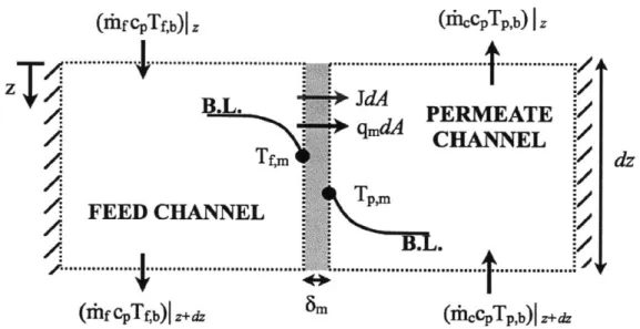
In AGMD, the condensation process is also integrated in the module, but with an air gap of thickness dgp on the order of 1 mm separating the coolant from the fresh water. In this case, seawater is also used as the coolant providing regeneration. An

AGMD module with the inflows and outflows as shown in Figure 2-4.

Taking a control volume surrounding each side of the membrane, the membrane itself, and the air gap/condensate channel, an energy and mass balance can be used to calculate all the necessary quantities. Figure 2-5 shows a control volume for one cell of length dz.

HEATED FEED IN B IE BRINE REJECT TO HEATER

tr

I

Figure 2-4: An AGMD membrane module with an integrated condenser.

(rfhfb)Iz

z~l

qmdA

A FEED CHANNEL

I

V

QC

V

TV

. .

..

dz

riicCp

Figure 2-5: A control volume of an AGMD module cell.

AIR

COOL-GAP ANT

I

The feed side and membrane are modeled as described the previous section. On the permeate side (air gap side), the partial pressure is a function of the mole fraction of water vapor present at the membrane surface and the total pressure on the permeate side, PP.

Pw,,,m = PXw,,,m (2.15)

In the case of the systems modeled here, P, is always atmospheric pressure. The mole fraction can be related to the common humidity ratio by Equation 2.16 [39].

XwIPIm = wp,m/0.622

(2.16)

1 + w,m/0.622

A control volume is taken around the air gap. Since the gap distance is very small

(dgap/Lm < 1 and dgap/wm < 1) convective flow, in the form of natural circulation, in the z direction is assumed to be negligible. The flow of permeate to the condenser surface is governed by binary diffusion across the gap as described by Equation 2.17 [40]:

Jm _ cD -a In

(1+

(2.17)

Mw dgap - J Xa,ml - 1

In this formulation, it is assumed that no mass is transfered back through the mem-brane so that the flow of water vapor through the memmem-brane is one way. With the temperatures of an MD process, it is unlikely that air will dissolve back into the water of the feed stream.

The flow of mass is dependent on the molar concentration, ca, in the gap. This is approximated by treating the vapor-air mixture as an ideal gas at the mean cell temperature:

Pa

Ca = "P (2.18)

aR(Ta,m + T)/2

Energy flow into the air gap is limited by membrane conduction as described by Equation 2.9. While there is some energy released by sensible cooling of the vapor

as it passes through the membrane and air gap, it is typically less than one percent

of the membrane conduction qm and a several orders of magnitude lower than the latent heat carried by the vapor. Therefore it is approximated to be zero. In the air gap, that energy is convected across the gap with the moving vapor, as described by Equation 2.20. Thermal radiation across the gap was considered, but found to have a negligible effect on flux and temperature, and was not included in this model. The convective heat transfer is easily derived by solving the energy equation where the convective velocity u is Jm/pmix:

dT d2_T

Ud = a (2.19)

dx dX2

where x in this case is the coordinate direction across the gap (not a mole fraction). Applying boundary conditions at the air side of the membrane (temperature and heat flux) and integrating twice the following equation is obtained:

Ta,m - TZ =

(m)

All fluid properties are for the air/vapor mixture at the specific temperature in each

cell.

The temperature of the condensate interface, T is determined by the partial pres-sure of water in air by solving Equation 2.2 at the interface where the mole fraction

xi is the ratio of the partial pressure of water vapor to the gap pressure Pa.

Upon entering the condensate layer the vapor gives up its latent heat, and the mass contributes to the thickening of the condensate layer. In gravity driven conden-sation, the layer thickness, 6, resists heat flow and is related to the mass of permeate

condensed by a simple laminar flow boundary layer equation [38]:

dhp= (P V)wM [(6 + d)3 - j3] (2.21)

3v,

The heat conducted through the condensate layer is the sum of the heat conducted through the membrane, q,,, and the latent heat given up through condensation, eval-uated at the interface temperature, Ti.

% = q. + Jmhf, (2.22a)

qc = k (Ti - Twall) (2.22b)

The condensate collects at the bottom of the module and the heat goes into the coolant stream. A boundary layer resistance in the coolant stream similar to that of the feed stream limits heat flow as described by Equation and 2.8. However, the heat that is absorbed into the condensate stream and passes through it's boundary layer is different, as no mass passes through the wall. The heat that enters the condensate stream is the sum of the membrane conduction, latent heat, and some sensible cooling of the liquid in the condensate layer.

rhcdhp,b = [qc + Jm(hw,i - hw,waii)] dA (2.23)

Boundary layer resistance is described by:

qc + Jm(hw,i - hw,wa ) = -ht,c(Tc,b - Twal₁) (2.24)

The heat transfer coefficient in the coolant stream, ht,,, is calculated in the same way as that of the feed stream. The thermal resistances are comparable because of comparable mass flow rate and flow channel size.

2.5

Pumped Vacuum MD System

A pumped vacuum system is the most common type of VMD system. It consists of

vapor extraction driven by a vacuum pump. Figure 2-6 show the flows in and out of a VMD module. HEATED FEED MD @ pI BRINE VAPOR TO REJECT CONDENSER

Figure 2-6: A VMD module where permeate is removed by a vacuum pump and condensed.

Unlike the AGMD system, where the air does not exit the system and can be main-tained at a constant pressure, the vapor flow is driven by a vacuum pump. The pressure that the pump can achieve is inversely proportional to the flow rate of vapor from the module. This is obtainable from a pump curve. Since the vacuum pressure of the pump curve is a function of the total flow rate, integration of the permeate mass flow through the entire module is needed to find the vacuum pressure. Therefore, iteration is required to find the actual pressure.

During startup, the pump removes any air sitting in the module at a high rate, and the pump reaches steady state operation. During steady state, mass conservation dictates that only water vapor that enters through the membrane is removed (no air

leaks in an ideal case). Figure 2-7 shows a schematic drawing of a startup transient.

0 *ri

o 1

---$4 " Vapor Mole Fraction I

na . I *0.8 0 0.4 0 2 Vacuum Pressure . O 0 20 40 60 Time

Figure 2-7: Schematic drawing of a startup curve showing the vacuum pressure and mole fraction of vapor on the permeate side of the module.

This model assumes that the process is running at a steady state such that:

Jm = B(pw,f,m - P) (2.25a)

Pf = PVm (2.25b)

From Pump Curve

The end result is that the flux is effectively dependent on the feed side temperature and the power of the pump. Since there is only vapor at reduced pressure on the permeate side, and the boundaries of the permeate chamber are adiabatic, no fogging is expected.

The feed side heat and mass transfer are calculated as described in the first section. However, on the permeate side there is no air at a lower temperature to conduct heat from the membrane, only vapor at Tj,m. As a result T,m ~ Tf,m and qm ~ 0. This is consistent with the very nearly isothermal expansion experienced by the water vapor as it passes through the pores, as the membrane thickness (minimum length of the pores) is about 1000 times the size of the nominal pore diameter. The heat flow that keeps the vapor isothermal, qexp, is conducted though the solid parts of the membrane, and it may be calculated from the change in vapor enthalpy, hv, using Equation 2.26:

qexp = Jm [hf,m + hfg - hv(P, Tf,m)] = RTf,m in (v'Pm) (2.26)

\ VV f,m /

This heat of expansion is subtracted from the heat removed from the feed side control

volume.

A boundary layer of moving vapor develops on the permeate side and the overall

enthalpy of the vapor stream increases with additional membrane flux. A control volume representing this process is shown in Figure 2-8.

(rif cpTb)| z _{1ivhv,blz Iilviz}

z

PERMEATE/

/FEED CHANNEL

PEMET

/ L

qmdA

VAPOR

CHANNEL

dz

Tf~m Tp~m

(Ilf CpTf,b) z+dz ilIvhv,bI z+dz Imy Iz+dz

Figure 2-8: Control volume of a VMD membrane module cell.

Since no species other than water vapor is present in the permeate channel in steady state there, no concentration gradient is present to resist mass flow. Hence, the enthalpies of the streams combine according to Equation 2.27:

(rihv,b)jz+dz = (?iphv,b)Iz + Jmhv,mdA (2.27a)

2.6

Solution Method and Verification

The discretized numerical model was typically made up of several hundred cells with a set of equations describing the interactions from the hot-side to the cold-side bulk conditions at each cell. The resulting system can be upward of 10,000 equations solved simultaneously. Each of the cells encompass a finite length, and mass and heat flows are described by a single quantity for that length. A sufficient discretization to accurately describe the membrane could be obtained by increasing the number of cells (decreasing dz for given length) and observing a change in the output. For the longest membrane length, or largest values of the differential dz, the solution did not change in excess of 1/2% after the number of cells was increased to 260.

2.7

Model Validation

Models were evaluated numerically using parameters published in experimental stud-ies of MD systems. The standard package Engineering Equation Solver [29] was used for calculations. Properties for pure water [371 were used and evaluated at the temperature and pressure of the bulk flows in each cell.

2.7.1

Direct Contact MD

Validation of the DCMD model was based on experiment done by Martinez-Diez and Florido-Diaz [35]. Table 2.1 shows given parameters provided as inputs for the model. The membrane distillation coefficient was not reported and was only implied by the experimental results, however for the purposes of validation, a value of B for the same type of membrane measured by Vazquez-Gonzalez and Martinez [36] was used.

Table 2.1: Operating parameters from Martinez-Deiz [35]. Starred parameters are compared with inodel for validation.

Given Parameter

Feed/Permeate Flow Rate

Feed Temp. (Inlet/Outlet Average) Permeate Temp. (Inlet/Outlet Average) Length

Channel Width Channel Depth Membrane Type

Membrane Distillation Coeff. (Measured, [36]) Permeate Flux* Value Various 45 *C 35 *C 55 mm 7 mm 0.4 mm

Gelman Inst. TF200 PTFE 22 x 10-7 kg/M 2 Pa sec

Various

Experiments were conducted [35] at three mass flow rates through the channel:

1.65 x 10-3 kg/s, 1.21 x 10-3 kg/s, and 0.772 x 10-3 kg/s. Table 2.2 shows the

experimental results compared to the model.

Table 2.2: Deiz [35].

Comparison between model presented here and an experiment by

Martinez-Run # Mass Flow Rate Permeate Permeate % Difference

Flux - Expt. Flux - Model From

Experi-ment 1 1.65 x 10-3 kg/s 10.08 kg/m2hr 16.28 kg/m 2hr 61.5% 2 1.21 x 10-3 kg/s 9.36 kg/m2_hr 16.05 kg/m 2hr 71.5% 3 0.772 x 10-3 kg/s 8.64 kg/m 2 hr 15.79 kg/m 2hr 82.7%

Given the simplicity of the DCMD system, presuming the accuracy of the module geometry and mass flow rate, the results suggest that the value of B is different from the one measured by Vazquez-Gonzalez and Martinez [36] (given in Table 2.1). If only an error in the membrane distillation coefficient is presumed, better agreement is obtained by reducing B to 13 x 10- 7. Additionally the spread in results between

each mass flow rate is greater than predicted by the model, with closer agreement at the higher mass flow rate. This suggests inconsistencies in the feed and permeate channel flowrate or channel geometry, and as a result inconsistencies in the temper-ature polarization, which can be a dominant resistance in DCMD, especially for low Reynolds number feed flows such as the ones in this study. With a small membrane

area, inconsistencies between runs could more dramatically affect the results and the local membrane distillation coefficient could be significantly different in a small membrane coupon vs. a large one due to manufacturing variability or fouling.

2.7.2

Air Gap MD

The Fath et al. [6] air gap system was a larger scale solar-heated installation. Its parameters are shown in Table 2.3. Data was given for the operating conditions and inlet/outlet temperatures over time. For the present comparison, a point in the middle of the day was selected to avoid the effect of startup transients.

Table 2.3: Operating parameters from Fath et al. [6]. Outlet temperatures and mass flow rates, denoted with an asterisk, are compared with the model for validation.

Known Parameters Value Approximated Value Parameter

Feed Flow Rate 0.14 kg/s Membrane Distilla- 16 x 10-7 kg/m2 _{Pa s}

tion Coeff.

Feed Inlet Temp. 72 *C Air Gap Width 1 mm

Condenser Inlet Temp. 45 0C Flow Channel 4 mm Width

Membrane Area 8 m2

Permeate Flowrate* 10 kg/hr

Feed Outlet Temp.* 50 *C

Condenser Outlet Temp.* 65 *C

Mean membrane distillation coefficient values for PTFE membranes were obtained from external testing [17, 34, 35]. The value used here represents an average value for commercially manufactured membranes. Measurements for the channel depth and air gap were made from a photo of the cross-section of the module and outer module dimensions [41]. With a mean condensate layer thickness 60 Am, the condensate layer thickness did not exceed 1/10th of the air gap, which is consistent with prior observation [14].

Table 2.4 shows the results of the simulation compared with the experiment. Er-rors are deviations from the experimental value. For calculating error all temperatures are temperature differences between the inlet and outlet.

Table 2.4: Comparison between simulation and Fath et al. experiment [6].

Quantity Experimental Simulated % Difference from Experiment

Permeate Flow Rate 10 kg/hr 9.38 kg/hr 6.2%

Feed Outlet Temp. 50 *C 49.3 *C 3.3%

Condenser Outlet Temp. 65 *C 67.4 *C 12.0%

The simulation approximates the flux and temperatures well, slightly over-predicting flux and temperature drop. The over-prediction of flux, which would lead to more en-ergy being taken from the feed stream, may be explained by the lack of non-idealities such as heat loss which would affect the channels on the outer-most surface of a spiral-wound module such as this. Also the presence of non-condensible gases and dissolved solids in the seawater would lower the partial pressure on both the feed and air gap sides, resulting in lower flux.

2.7.3

Pumped Vacuum System

While there have been no pilot-scale VMD systems similar to the Fath et al. air gap system, recent experiments have been conducted on smaller bench-top setups. One such setup is a flat sheet system developed by Mericq et al. [42]. Several experiments were conducted with varying salinity brines, including RO retentate. Table 2.5 shows parameters from the lowest salinity experiment with a salt concentration of 38,000 ppm. Fluxes were measured initially and over time to account for fouling of the membrane. The initial flux value is used for comparison as the model does not account for fouling.

The heat transfer coefficient has been calculated from the channel geometry and known flow rate and Reynolds number.

The resultant flux was 10.43 kg/m 2hr, 3.2% greater than the initial value measured in the experiment. Since the simulation used pure water properties, there will be a difference of flux due to the reduction in partial pressure of the water vapor and reduction in specific heat capacity [43]. However, an analysis of a VMD module based on the pilot-scale dimensions in Table 2.3 using seawater properties and varying the

Table 2.5: Operating parameters from Mericq et al. [42]. Parameters denoted with an asterisk are compared with the model for validation.

Known Parameters Value

Feed Flow Rate 0.0366 kg/s

Feed Inlet Temp 53 *C

Permeate Side Pressure 7 kPa

Membrane Area 57.75 cm2

Channel Depth 1 mm

Membrane Distillation Coeff. 4.37 x 10-7 kg/M2 Pa s

Feed Side Heat Transfer Coeff. 7809 W/m2K Permeate Flux* 10.1 kg/M2 hr

salinity shows that the flux decreases 3% as the salinity increases by 45,000 ppm from

0, which is within the uncertainty in the experimental results.

2.7.4

Membrane Distillation Coefficient Data

The membrane distillation coefficient has a large impact on the flux and, due to the non-uniform nature of MD membranes, it is difficult to determine exactly.

The membrane distillation coefficient, B, is primarily a function of the membrane material properties, the pore size, the vapor being passed through the membrane, and a weak function of temperature. Flow is controlled by two diffusion processes, Knudsen, and molecular diffusion, which depend on the pore size relative to the mean free path of water molecules as given by Equation 2.28:

A = (2.28)

v2'7rPpoI2

The mean free path is dependent on pressure and temperature. P,, the sum of the partial pressures, is the total pressure in the membrane pore, and is equal to the pressure on the permeate side at all times and positions. Formulations for each process [44] can be described using Equation 2.29:

2 gr (8 M 1/2 BK - 2(2.29a)