HAL Id: hal-00316239
https://hal.archives-ouvertes.fr/hal-00316239
Submitted on 1 Jan 1997
HAL is a multi-disciplinary open access
archive for the deposit and dissemination of sci-entific research documents, whether they are pub-lished or not. The documents may come from teaching and research institutions in France or abroad, or from public or private research centers.
L’archive ouverte pluridisciplinaire HAL, est destinée au dépôt et à la diffusion de documents scientifiques de niveau recherche, publiés ou non, émanant des établissements d’enseignement et de recherche français ou étrangers, des laboratoires publics ou privés.
First results from the plasma composition spectrometer
PROMICS-3 in the Interball project
I. Sandahl, S. Barabash, H. Borg, E. Yu. Budnik, E. M. Dubinin, U. Eklund,
H. Johansson, H. Koskinen, K. Lundin, R. Lundin, et al.
To cite this version:
I. Sandahl, S. Barabash, H. Borg, E. Yu. Budnik, E. M. Dubinin, et al.. First results from the plasma composition spectrometer PROMICS-3 in the Interball project. Annales Geophysicae, European Geo-sciences Union, 1997, 15 (5), pp.542-552. �hal-00316239�
Ann. Geophysicae 15, 542—552 (1997) ( EGS — Springer-Verlag 1997
First results from the plasma composition spectrometer PROMICS-3
in the Interball project
I. Sandahl1, S. Barabash1, H. Borg1, E. Yu. Budnik2, E. M. Dubinin2, U. Eklund1, H. Johansson1, H. Koskinen3, K. Lundin1,
R. Lundin1 , A. Mostro~ m1 , R. Pellinen3 , N. F. Pissarenko2 , T. Pulkkinen3 , P. Toivanen3 , A. V. Zakharov2
1 Swedish Institute of Space Physics, PO Box 812, S-981 28, Kiruna, Sweden 2 Space Research Institute, Profsoyuznaya 84/32, 117 810 Moscow GSP-7, Russia 3 Finnish Meteorological Institute, PO Box 503, SF 00 101 Helsinki, Finland Received: 3 January 1996/Revised: 13 May 1996/Accepted: 27 May 1996
Abstract. PROMICS-3 is a plasma experiment flown in the Russian project Interball. It performs three-dimen-sional (3D) measurements of ions in the energy range 4 eV—70 keV with mass separation and of electrons in the energy range 12 eV—35 keV. The Interball project consists of two main satellites, the Tail Probe and the Auroral Probe, each with one subsatellite. The Interball Tail Probe was launched on 3 August 1995, into a 65° inclina-tion orbit with apogee at about 30 RE. Both main satel-lites carry identical PROMICS-3 instruments and thus direct comparisons of the particle distributions will be possible once the Auroral Probe is launched. Further-more, PROMICS-3-Tail is the first instrument measuring the 3D ion distribution function in the magnetospheric boundary layers at high latitudes. In this paper we describe the PROMICS-3 instrument and show initial results from the Tail probe, measurements of the mag-netosheath, plasma sheet, and ring current plasmas.
1 Introduction
The Interball project is designed to study mechanisms responsible for the transport of solar wind energy, mass, and momentum to the Earth’s magnetosphere as well as the accumulation and dissipation of these entities. In particular, this includes the study of processes involved in magnetospheric substorms. During its lifetime, the Inter-ball Tail probe will visit all local time sectors, thus provid-ing measurements from several locations in the plasma sheet and the magnetospheric boundary layers. The Auroral probe will make measurements above the high-latitude ionosphere, using both in-situ and imaging tech-niques. The Tail Probe was launched on 3 August 1995 and at present the Auroral probe is still waiting to be
Correspondence to: I. Sandahl
launched. A presentation of the Interball project is given by Galeev et al. (1995).
During the past few years it has become increasingly clear that in order to understand many magnetospheric processes we need multi-point measurements in space. In the field of hot plasma particle measurements it has been realized that crucial information is contained in the full three-dimensional (3D) particle distribution, as well as in the separation of the different particle species. The PROMICS-3 experiment addresses all these questions. PROMICS is an acronym for Prognoz Magnetospheric Ion Composition Spectrometers, since earlier instruments by the same team were flown on the Soviet satellites Prognoz 7 and Prognoz 8. But while these earlier instru-ments, PROMICS-1 and PROMICS-2, only measured in two viewing directions with respect to the satellite spin axis and missed the sunward streaming plasma, PROMICS-3 measures the full 3D distribution function. In addition, PROMICS-3 has a larger energy range. PROMICS-3 performs simultaneous measurements of ion and electron distribution functions, moments, and plasma composition both above the auroral ionosphere and in the magnetotail with identical spectrometers. The instruments are the result of a cooperative effort between the Swedish Institute of Space Physics, IRF, in Kiruna, the Space Research Institute, IKI, in Moscow and the Finnish Me-teorological Institute, FMI, in Helsinki.
With its apogee near 30 RE and inclination about 65°, Interball will probe the high-latitude boundary layers over long time periods. PROMICS-3-Tail will be the first ion mass spectrometer making full 3D distribution func-tion measurements in this region. Earlier ISEE 3 results revealed that there are often bi-directional electron beams in the tail lobes (Baker et al., 1986; Gosling et al., 1985). These beams were considered to be formed of electrons entering the magnetosphere from the solar wind through the locally open magnetotail, and to form the population that at low altitudes has been identified as the polar rain within the polar cap. Later, Geotail measurements showed that these bi-directional electrons are accom-panied by relatively low-energy ion beams, which seem to
originate from the high-latitude ionosphere. Such ion beams have earlier been observed at low altitudes by Viking and Akebono in the cleft region (Thelin et al., 1990; Nishida, 1992). Low-altitude bi-directional electron beams are normally associated with ion conics (Thelin and Lundin, 1990) that subsequently fold into beams further out along the field lines. With PROMICS-3-Tail, we will be able to study the entry mechanisms of the particles through the high-latitude magnetopause (Lundin, 1988), and to study both the ion and electron signatures in the tail, whereas PROMICS-3-Auroral can probe the up-ward flowing ions and the polar rain. Furthermore, in advantageous constellations of the two spacecraft, we may even be able to relate the populations seen in the tail to those seen at the conjugate point above the polar regions. During the latter part of 1995, the Interball apogee was near the tail center. In November and December of 1995 particularly, there were several interesting passes during which Interball traversed the central plasma sheet very close to the nominal neutral sheet from distances beyond 30 RE to the ring current region inside geostationary orbit. These regions have been identified to be the key regions for the substorm process: The current sheet disruption events are frequently observed inside of about 10 RE (e.g., Lui, 1991), whereas the neutral line is assumed to form typically in the region between 15 and 30 RE (Baum-johann et al., 1989; Baker et al., 1996). Observations and theoretical arguments suggest that both of these processes involve the formation of a thin and intense current sheet during the substorm growth phase (Sanny et al., 1994; Pritchett and Coroniti, 1994). However, it is not clear whether these processes evolve independently within lo-calized current sheets or are local signatures of the inner and outer portions of a large-scale thin and intense cur-rent sheet. With PROMICS-3, we will be able to study the particle motions within the neutral sheet in both of these regions, and thus address the questions about the scale size of the thin current sheet and the temporal sequence at the late growth phase and early expansion phase.
Increased levels of O` ions in the near-Earth magneto-tail have been suggested to play a role in substorm dy-namics (Baker et al., 1982; Cladis and Francis, 1992). Enhanced oxygen populations have been detected earlier with AMPTE/CCE during multiple substorms and during strong substorm growth phases (Daglis et al., 1994). Daglis et al. (1994) concluded that in multiple substorm events, the oxygen content enhances after the first breakup, and remained at an enhanced level during the subsequent substorms or substorm activations. However, the significance of these observations to the onset mecha-nism or growth phase time scale is as yet unknown. With PROMICS-3, we can probe the oxygen content of the central plasma sheet over periods lasting several hours during the tail passes, which gives a good opportunity to study its significance to the dynamics of substorms.
The ion dynamics both at the high-latitude boundaries and within the plasma sheet has received considerable attention recently. Several statistical studies have revealed that the plasma sheet is in a turbulent state, from which the average convection pattern is formed only after heavy averaging over almost randomly distributed velocity
vec-tors (e.g. Angelopoulos et al., 1992). Furthermore, theoret-ical studies of ion trajectories in the plasma mantle and plasma sheet have shown that the non-adiabaticity of the ion motion in most parts of the tail (outside the quasi-dipolar, near-Earth region) does have an effect in the large-scale configuration and pressure distribution of the tail plasma sheet (Ashour-Abdalla et al., 1991; 1993). The full 3D distribution functions from PROMICS-3 together with several magnetic field experiments on board Interball can provide valuable information about how the plasmas are organized in the plasma sheet at various distances.
Having identical instrumentation at high and low alti-tudes allows us to establish field-line mappings in regions where the particle spectra are similar. Using DMSP and the LANL geostationary satellite data, Reeves et al. (1995) have demonstrated that for many cases, a spectral match between high-altitude and low-altitude satellites lasts only a fraction of a minute. In such occasions, at the time for the spectral match it can often be assumed that the two satellites are on the same field line, thus providing a direct, observational mapping between high and low altitudes. This method can be important for future development of magnetic field modelling capabilities.
This work gives a brief introduction to PROMICS-3 and describes the first scientific results from the Tail Probe. A more detailed presentation of the instrument can be found in Sandahl et al. (1995) and an extensive descrip-tion including all calibradescrip-tion constants and constants for the detailed moment calculation is in preparation and will be issued as an IRF report.
2 PROMICS-3 basic design
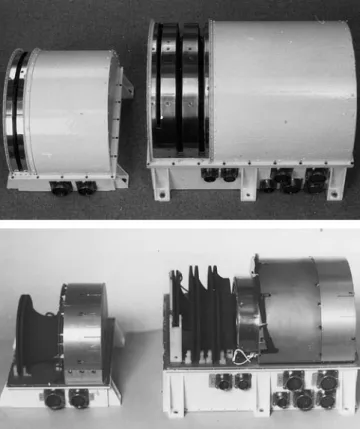
Each PROMICS-3 instrument consists of two units, MEPS (magnetospheric electron spectrometer) for elec-tron measurements in the energy range 12 eV—35 keV and TRICS (3D ion composition spectrometer) for positive ion measurements with mass separation in the energy range 4 eV—70 keV. PROMICS-3 measures the 3D distri-bution functions of electrons and up to six positively charged ion species. Photographs of the instrument units are shown in Fig. 1.
The basic design principle of MEPS is shown in Fig. 2. The electrons enter the instrument through one single toroidal electrostatic analyzer with a total opening angle of 180° and a deflection angle of 127°. Behind the analyzer eight detectors are arranged in a fan-like fashion, each one recording electrons from an analyzer sector of approxi-mately 35°. There is some overlap between the fields of view of the different sensors, as shown in Fig. 3. The satellite spin axis is horizontal in the figure and thus the full unit sphere is covered during one spin. The MEPS detectors are numbered D12 to D19 as shown in Fig. 2. The spin axis points towards the Sun and D12 is the most sunward-looking detector.
In order to minimize noise, each sensor is placed in a closed compartment. The sensors are Mullard X955 BL channel electron multipliers. Thermal electrons are ex-cluded by grids with a voltage of !12 V in front of the electrostatic analyzer and the CEM compartments. The
Fig. 2. Basic design principles of MEPS Fig. 1. PROMICS-3. The electron spectrometer MEPS is to the left
and the positive ion spectrometer TRICS is to the right. The lower photograph shows the instrument with covers removed. Note the
stacked design of the three TRICS toroidal electrostatic analyzers Fig. 3. Calibrated field of view of MEPS-Auroral voltages of the electrostatic analyzer plates are
symmetri-cal so that the potential halfway between the plates is approximately zero.
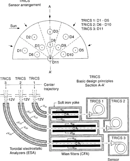
The design of TRICS is quite similar to MEPS and is outlined in Fig. 4. In order to obtain a good dynamic range as well as a high sensitivity at all energies this unit is divided into three subunits with different energy ranges. TRICS-1 and TRICS-2 contain five detectors each and TRICS-3 consists of one detector. These detectors are
numbered D1 to D11 as shown in Fig. 4. Detectors 5 and 10 have their viewing directions closest to the Sun. Each TRICS subunit consists of a toroidal electrostatic ana-lyzer followed by Wien velocity filters with crossed electric and magnetic fields. All detectors of each subunit share the same toroidal analyzer, but have separate Wien filters. In order to keep the size and weight of the instrument down, the subunits are stacked, making maximum use of the instrument volume. TRICS also contains a data proces-sing unit, DPU, with a SBP9989 processor serving both TRICS and MEPS. The DPU performs all onboard calculations in real time and also carries out instrument control.
In TRICS-2 and -3 the voltages of the electrostatic analyzer plates and the Wien filter electrostatic plates are symmetrical giving a zero center potential between the plates. In TRICS-1, the subunit for the lowest energy range, the center potential is !12 V in order to avoid particles with nearly zero energy in the instrument. Since
Fig. 4. Basic design principles of TRICS
the ion detection efficiency of the sensors is poor for energies below a few kilovolts, all TRICS sensor openings have a negative potential of at least 2.5 kV.
Figures 5 and 6 show some examples of the perfor-mance of TRICS. In contrast to MEPS, there is very little overlap between the sectors measured by the different detectors. This is demonstrated in Fig. 5, which shows the calibrated opening angles of TRICS-2-Tail. Figure 6 shows the mass resolution at 12 keV of TRICS-3-Tail.
A summary of the instrument characteristics is given in Table 1.
3 Measurement and telemetry modes
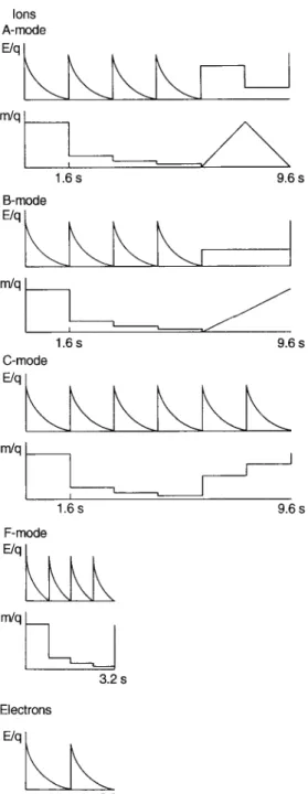
The ion spectrometer TRICS can be operated in four different measurement modes denoted A, B, C, and F. The electron spectrometer MEPS is operated in only one mode. The measurement modes are described in Fig. 7. A complete measurement cycle for ions is completed in about 9.6 s in modes A, B, and C giving 12 cycles per spin. In the fast mode F and for the electrons, the duration of a measurement cycle is about 3.2 s. The onboard software distributes the measurement cycles evenly around each spin revolution of the satellite.
Mode A is the default mode. Each 9.6-s cycle begins with energy spectra of 32 energy levels at four fixed mas-ses. After that 32 level mass spectra are obtained at two fixed energies. The sampling time at each level is 43.7 ms and the sweep time for each spectrum is 1.6 s. Since TRICS consists of three subunits sweeping three energy ranges simultaneously, the total number of energy levels is 96. The fixed mass and energy levels can be selected by commands. The default mass levels correspond to H`, He``, He`, and O` and the default energy levels are 0.1, 0.6, 1.6, 5.4, 11, and 33 keV.
The first part of the mode B cycle is identical to mode A. The only difference is that the mass spectrum contains 64 mass levels and is obtained during 3.2 s for one mass only.
In mode C, no mass spectra at all are measured. Instead energy spectra are measured for six fixed masses.
Mode F is designed for boundary crossings and other circumstances when a high temporal or spatial resolution is desired. Energy spectra of 0.8 s and 16 energy levels are measured at four fixed masses. This mode can only be used together with the direct telemetry mode described later.
The electron measurement cycle consists of a total of 64 energy levels that are stepped through during two
Fig. 5. Calibrated field of view of TRICS-2-Tail
Fig. 6. Mass resolution of TRICS-3-Tail at 12 keV
Table 1. Summary of instrument characteristics
MEPS TRICS
Particle species: Electrons Ions 1—56 amu, mass separation
Weight (kg): 3.2 12.6
Power cons. (W): 2 11
MEPS TRICS-1 TRICS-2 TRICS-3
Energy range (keV): 0.01—35 0.004—1.5 1—30 5—70
Number of sensors: 8 5 5 1
Total field of view (degrees): 3]180 10]180 4]180 2]48 Field of view per sensor: 3]35 10]36 4]28 2]48 Geometric factor at 1 keV (cm2 sr): 6]10~5 9]10~4 6]10~5 1]10~5
DE/E (FWHM): 0.07 0.20 0.10 0.06
M/DM (FW) for H`: 3 (1 keV) 9 (6 keV) 16 (12 keV)
Calculated moments: Density, mean velocity vector, pressure tensor, energy flux. Temporal resolution: 120 s ("one spin) for full distribution (240 s in slow mode). Data production rates
Direct transmission: 1900 bps,
Tape recorder: 16 bps (slow), 40 bps (medium), 384 bps (fast), 1900 bps(Same as direct transmission).
consecutive sweeps. Sweep number one measures the flux at even and sweep number two at odd energy levels. Due to the small energy bandwidth of the spectrometer, a 32 level sweep leaves gaps in the energy coverage, but these gaps are covered by the following sweep. This procedure was adopted because it is known that electron energy distributions sometimes contain very narrow peaks. On the other hand, less dramatic distribu-tions can here be measured with a higher time resolution than what would have been possible with a single 64 level sweep.
Due to telemetry and data storage limitations, it is not possible to transmit all the data obtained. Therefore, a rather complicated scheme of onboard data selection has been developed, which includes data compression as well as averaging and moment calculations. The output data production rate for the four possible telemetry modes are given in Table 1. The tape recorder mode bitrates thus denote the rate at which PROMICS-3 sends data to the tape recorder. Algorithms for the data selection have been defined for each possible combination of instrument mode and telemetry mode and is included in the onboard software. In the three-letter mode acronyms, the first letter (A, B, C, or F ) denotes the instrument mode and the last (D, S, M, or F ) the telemetry mode. The data selection algorithms are essentially fixed, but some minor modifications can be carried out by commands from the ground, for example changes of inte-gration limits, mass and energy tables or intercalibration factors, or exclusion of an entire detector from the moment calculation.
In the tape recorder modes, the available data storage space for PROMICS-3 is 16 Mbit. This space is filled up in 11.6 h by the fast mode or in 112 h by the medium mode. The longest tape recorder sessions last for about 4 days. It is thus necessary to plan the data taking very carefully in advance.
Fig. 7. Ion and electron measurement modes
4 Output parameters
The telemetered data from PROMICS-3 is a combination of energy spectra, mass spectra, and moments. In the direct telemetry mode the telemetry stream contains en-ergy and mass spectra with a good resolution and the moments can be calculated from this information on the ground. In the slow mode, on the other hand, more than one third of the telemetry capacity is devoted to onboard calculated moments. The moments are given with a time resolution of two spins, or about 240 s. The energy spectra are averaged down to eight energy levels per subunit, giving ion spectra of 24 levels. The energy spectra are also
averaged over a combination of different detectors and spin phase angles, so that the final result represents the mean spectrum over a part of the unit sphere. The unit sphere is divided into 3, 4, 6, or 16 sectors, depending on the mode. Just as in the case of the slow mode, the telemetry format during medium and fast modes contains a combination of moments and spectra, but with better temporal and better energy resolution.
5 Flux and moment calculation
The physical unit actually measured by PROMICS-3 is the count rate R(¼,b, /), where ¼ is the particle energy, b the angle between the spin-axis and the spectrometer orientation, and/ the azimuth angle given by the space-craft spin phase. The differential directional flux j is ob-tained from the count rate given in counts per second from
j (¼,b, /)"R(¼,b, /)
Ck (cm2 s sr keV)~1. (1) Ck is the conversion factor for detector k which has been
determined by calibration. The conversion factor can be expressed as
C(¼, k)"Gkg¼"(ifk)~1G0g¼ (cm2 sr keV). (2) Here ifk is the intercalibration factor for detector k, G the geometric factor in cm2 sr for the most sensitive detector of the subunit, h the absolute efficiency of the channel electron multiplier for the particle species to be measured and ¼ the energy in keV. The values of ifk range between 1 and 2 and mainly depend on geometrical differences between the sectors.
The absolute efficiency function h for electrons is ap-proximated by g"0.327#15.318 ¼!133.93 ¼2 ¼(50 eV, g"0.632#2.8232 ¼!8.1718 ¼2 50 eV4¼(200 eV, (3) g"0.89
A
1! 2 3# 8.5 (¼!0.1)B
200 eV4¼.This approximation of the efficiency function has been obtained by calibration at IRF and it closely follows the function given in the Electron Multipliers Data Hand-book (Philips Components, 1990) for energies below 3 keV. For higher energies, the above equation gives a somewhat lower efficiency.
For ions, an approximation derived from the efficiency curve given in the Electron Multipliers Data Handbook is used. The ion efficiency ranges between 0.4 and 0.8.
The plasma moments calculated by PROMICS-3 are the number density N, the mean flow velocity u
6 the mo-mentum flux tensor P
1, and the energy fluxe6. Separate ion moments are calculated and telemetered for each of the three TRICS subunits. For TRICS-1, however, the energy levels overlapping with TRICS-2 have been excluded from
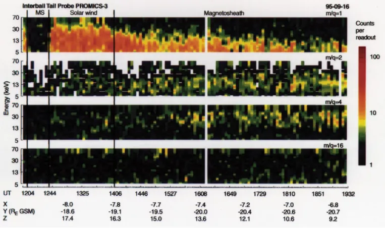
Fig. 8. Ions of different species measured on 16 September 1995 in the dawnside magnetosheath just inside the bow shock had energies proportional to the mass per unit charge
the integration in order to facilitate the calculation of the total moments from TRICS-1 and -2. In the electron moments, the contribution from photoelectrons is avoid-ed by excluding the energies below 70 eV.
6 First results
6.1. Observations in the dawnside magnetosheath
6.1.1 Ion composition at the bow shock in a compressed magnetosphere
Figure 8 shows an inbound pass through the dawnside magnetopause and magnetosheath on 16 September 1995, between 1204 and 1900 UT. During this period, Interball Tail Probe went from 27 to 24 RE in radial distance. Judging from Kp, the magnetic activity was moderate to low (values between 3 and 1#), but despite this the data from TRICS-1 and the FM-3I magnetometer show that the spacecraft was outside the bow shock both before 1210 UT and between 1240 and about 1410 UT. The compression may have been caused by a high solar wind density. Between 1210 and 1240 UT a temporary expan-sion of the magnetosheath engulfed Interball Tail and around 1410 the spacecraft again entered the mag-netosheath.
PROMICS-3 was in the AEM-mode, which is the slowest mode normally used. The data in the figure are from TRICS-3 and are in this mode averaged over two
satellite spins (240 s) into 8 energy bins. TRICS-3 accepts ions from a sector of about 50° centered approximately perpendicularly to the sunward direction.
The four panels show four different ion species; from top to bottom protons, alpha particles, He`, and O` in the energy range 5—70 keV. The count rates are not high, the maximum being only about 30 counts per readout, which corresponds to a flux of a few 104 (cm2 s sr keV)~1, but still a very interesting pattern is revealed. At 1240 UT, just after the retreat of the temporary magnetosheath expansion, the satellite encountered protons with energies of up to 30 keV and sometimes even more. Bursts of simi-lar protons appeared also before the part of the pass shown in the figure, but the onset at 1240 UT was more abrupt. It is not known how protons in the solar wind can gain such high energies. Classical pickup processes are only able to give a factor of four energy increase. One possibility is that the ions had originally been reflected from the bow shock and then gone through pickup acceleration.
After 1408 UT the upper energy threshold of these protons began to drop and soon afterwards increased fluxes of both alpha particles and He` ions appeared. This coincided with the reentry of the satellite into the mag-netosheath. The average energy of the alpha particles was about 15 keV, while the He` ions had higher energies, on average about 30 keV. In the oxygen panel, no corre-sponding population was measured. However, for the doubly and singly charged helium ions, the energy was proportional to the mass per charge. If this were true also
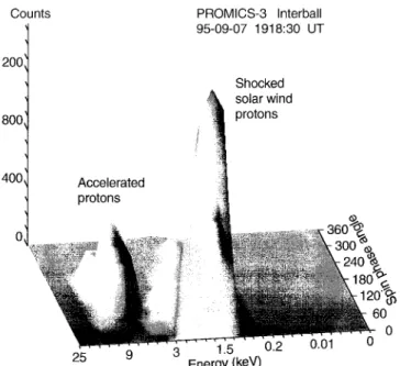
Fig. 9. Proton distribution measured in the dawnside mag-netosheath at about 30 RE (GSM coordinates: !6.8, !23.2, 18.7) on 7 September 1995 at 1918 : 30 UT. There were two distinct popu-lations, shocked solar wind protons with a peak at about 1.5 keV and accelerated protons with a peak at about 8— 9 keV
for oxygen, the average energy of oxygen ions would be about 120 keV, which is above the energy threshold of the instrument. There are, in fact, some counts in the highest energy channel, which could be the low-energy tail of such a population.
We tentatively interpret the He` and O` ions as being of ionospheric origin. However, the ordered energy rela-tionship suggests that alpha particles have become mixed with these before going through the same acceleration mechanism, for example ion pickup. It is, however, quite puzzling that high-energy protons were present in the solar wind and not in the magnetosheath.
In principle the ions of m/q+4 could also be heavier solar wind ions of a higher charge state, for example C4`, O5`, O6`, or Fe12`. This would imply a fast solar wind stream, but if that were the case there would also be very large fluxes of 5—6 keV protons. Since the proton flux was not very much larger than the flux of heavier ions, we rule out this alternative.
6.1.2 Proton distribution in the magnetosheath
During the beginning of the Interball mission the satellite orbit crossed the morningside magnetosheath and went out into the solar wind. Figure 9 shows a proton distribu-tion measured in the magnetosheath on 7 September at 1918: 30 UT at a distance of about 30 RE from the Earth. The data were obtained by TRICS-1 and TRICS-2 and the instrument was in the fastest possible mode, the FED mode. The plot shows the total number of counts in each energy step from D1 to D5 (TRICS-1) and from D6 to D10 (TRICS-2) as a function of spin phase angle. No heavier ions were detected. This was a day of moderate geomagnetic activity, Kp"3—4.
Two separate populations can easily be distinguished. The highest peak was centered at 1.5 keV and at a spin phase angle of 90°. It was mainly seen in detectors 5 and 10, which are the most sunward-looking detectors. Since it was also confined to a limited range of spin phase angles it has the character of a tailward steaming plasma. We interpret this population as shocked solar wind plasma.
The second population had higher energy, 8—9 keV, and appeared at spin phase angles of about 180°. Most of it was measured by detector D9 which has its viewing direction centered about 54° from the Sun. This popula-tion is probably related to accelerapopula-tion processes at the bow shock. There is a wide variety of suprathermal ion distributions in the bow shock and magnetosheath: reflec-ted ions, field aligned beams, diffuse protons, gyrophase-bunched and intermediate distributions (Fuselier, 1994). To distinguish between these populations a more detailed analysis of ion distribution functions together with mag-netic field data is necessary. Here, this example is present-ed to illustrate the capability of the instrument for such types of studies.
6.2 Observations in the magnetotail
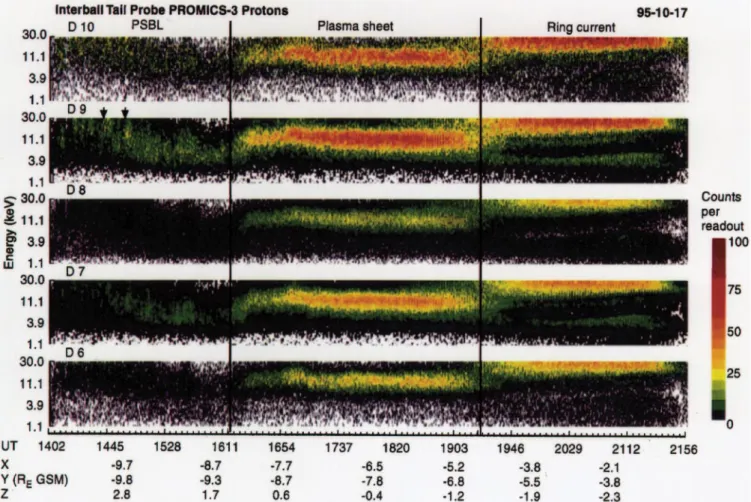
6.2.1 A traversal of the magnetotail from 15 to 4 RE During the inbound part of the orbit Interball spends several hours fairly close to the equatorial plane and it is thus possible to study the plasma sheet and surrounding regions. During October these traversals began in, or close to, the dawnside magnetosheath about 20—25 RE downtail. Figure 10 is a spectrogram obtained on 17 October between 1402 and 2156 UT. During that time, the satellite travelled from about 15 RE to about 4 RE. Figure 11 shows the trajectory in the xz and xy planes of the GSM coordinate system. The heavy lines give the actual spacecraft position and the thin line the projection along the field lines to the current sheet center according to the Tsyganenko 1989 (Kp) model.
The magnetic acitivity on this day was moderate. There seems to have been substorm activity earlier in the day (Kp"3 and 4), but the afternoon and the evening were relatively quiet (Kp"2 and 1).
PROMICS-3 was during this time in the AEF mode. The data in Fig. 10 were obtained by TRICS-2. The top panel shows the most sunward-looking detector, the middle panel the detector looking perpendicular to the spin axis, that is approximately in the GSM xy plane, and the bottom panel the most tailward-looking detector.
From the beginning of the spectrogram until about 1615 UT, fluxes were rather low with a decreasing average energy. In D9, a few very localized bright spots appeared, indicating the presence of strongly collimated beams. This whole region has properties typical of the plasma sheet boundary layer and we identify it as such. In Fig. 11, a finely hatched line has been used to mark it. It is interesting to note that this region here is very wide, more like a region in its own right than just a boundary. In fact, some examples given by Eastman et al. (1984) also show quite a wide PSBL.
Fig. 10. Spectrogram obtained during a traversal of the magnetotail on 17 October 1995. The intensity scale is counts per readout, which is approximately proportional to the energy flux. The accumulation
time for detectors D7 and D9 is twice as long as for D6, D8, and D10. ¹wo arrows above the second panel mark field-aligned beams
In this part of the orbit, the magnetic field lines should have an angle with respect to the Sun-Earth line of about 45° and field-aligned beams, if present, should be seen in D9 and D7. This is also what we observe. Two tailward-streaming, field-aligned beams are indicated by two arrows above the second panel.
At about 1615 UT the plasma characteristics changed to what is relatively normal in the plasma sheet. The intensity and the average energy increased. Most ions had energies between a few keV and about 15 keV. The distri-butions had no dramatic features and at the resolution of the plot no strong variations were measured as the satel-lite moved Earthward. The neutral sheet was crossed, but no signature of this was left in the particle data. In Fig. 11, the plasma sheet is marked by a solid line.
The plasma sheet population was left at about 1920 UT close to the geostationary orbit distance. This is a normal location of this boundary. As expected, the most energetic plasma sheet ions disappeared tailward of the less ener-getic ones. The satellite now entered the ring current region with much higher ion energies than before. Only the low-energy portion of the ring current population is within the energy range of the instrument. The ring cur-rent part of the orbit is drawn as a hatched line in Fig. 11. Here an interesting feature is the low energy population of about 3 keV. It only showed up in the three middle
detectors and was thus flowing in the cross-tail direction. These ions could be low-energy plasma sheet ions, which can drift closer to the Earth than ions of a higher energy. Figure 12 shows the result of a model calculation of the drift paths of ions with an original energy of 0.5 keV at a distance of x"!13 RE in the tail. The cross-tail electric field was assumed to be 0.1 mV/m and the original pitch angle 45°. The plot shows that such ions are able to reach the regions where the 3 keV ions were found. While drift-ing these ions increase their energy to about 4 keV. 6.2.2 Ring-shaped distribution of protons
in the plasma sheet
It has been known for some time that particle distribution functions in the plasma sheet are often very complicated. An example of a ring-shaped proton distribution with phase-bunching, obtained by TRICS-2 in the dawnside plasma sheet, is shown in Fig. 13. This distribution was encountered during an inbound pass at 0140 UT on 21 September at a distance of about 13 RE close to the equa-torial plane (SM coordinates !3.5, !13.1, !2.8). The magnetosphere had been rather quiet for several days. The upper part of the figure gives the angular distribution in a Mollweide projection. In this projection the surface elements have the correct relative size. The ‘‘latitude’’ corresponds to the angle with respect to the spin axis and
Fig. 11. The trajectory of Interball in GSM coordinates during the time of the spectrogram in Fig. 10. The thin lines show the projec-tions to the current sheet along the geomagnetic field lines according to the Tsyganenko model
Fig. 12. Drift trajectories of protons with an initial energy of 0.5 keV and pitch angle 45° in a dawn-dusk electric field of 0.1 mV per meter. Such particles may be the source of the 3 keV population occurring simultaneously with the ring current in Fig. 10
Fig. 13. Ring-shaped proton distribution with gyro bunching meas-ured on 21 September at 0140 UT in the dawnside plasma sheet (SM coordinates: !3.5, !13.1, !2.8). The upper part shows the total number of protons in the energy range 1—30 keV as a function of direction of incidence. The lower part shows a spectrogram mea-sured by D9 during one spin. This spectrogram constitutes the contribution from D9 to the upper part of the figure. The scale applies only to the lower part
the ‘‘north pole’’ points toward the Sun. The ‘‘longitude’’ gives the spin phase angle. The color scale shows the integrated number of counts from all energy levels in each direction bin. This procedure seems acceptable, since the energy spectra are similar to each other and do not con-tain significant peaks. An example of this, the contribution from D9, is shown in the lower part of Fig. 13.
The ring-like distribution of protons is clearly seen. The distribution along the ring is not uniform and the exist-ence of gyro-bunching may be observed.
Three-dimensional measurements of proton distribu-tions in the plasma sheet have been carried out earlier. Ring distributions and partial ring distributions were found by Nakamura et al. (1991). Frank et al. (1994) measured the 3D distribution function of protons in the Earth’s magnetotail during the passage of the Galileo spacecraft, demonstrating that Maxwellian distributions often did not describe the particle populations adequately. These authors presented cases of tailward flows with ring-shaped distributions. As in the case presented here, the angular distribution around the ring was asymmetrical and resembled several gyro-bunched beams. Ring-shaped velocity distributions of protons were observed also by Geotail at the plasma sheet-lobe boundary in the mid-tail
region (XGSM"!70 RE) and in the deep tail XGSM" !
120 RE) (Saito et al., 1994). These complex velocity distributions are likely to arise due to nonadiabatic motion of the ions in the tail current sheet (Speiser, 1965; Ashour-Abdalla et al., 1992, 1993).
7 Conclusions
The plasma spectrometer PROMICS-3 onboard Interball Tail Probe is working well and has already produced large amounts of interesting data. The early autumn 1995 and midwinter 1995/96 covered the dawn and dusk flanks, respectively, whereas passes in November covered the central tail. Good cusp passes were obtained in January and February 1996, and it is expected that spring and summer passes will bring interesting observations of the dayside. The studies are benefiting from the 3D capabili-ties of the PROMICS-3 instrument, and results will be reported in the near future. The tail passes during Novem-ber—December 1995 have initiated several studies of tail dynamics during disturbed periods and other ongoing studies concern the dawnside magnetosheath and bow shock. These studies involve other ISTP spacecraft also, and will be reported elsewhere. Interball and other ISTP spacecraft are opening up the possibility of disentangling some of the still-unresolved issues in magnetospheric physics.
Acknowledgements. The major part of the hardware has been
de-signed and built at the Swedish Institute of Space Physics in Kiruna. Much of the electronics has been built in Finland by the Finnish Meteorological Institute, Hollming OY, and VTT. PROMICS-3 is financed by grants from The Swedish National Space Board, the Technology Development Center (in Finland) and the Academy of Finland. The magnetometer data were kindly provided by M. Noz-drachev. We wish to thank the referees for helpful comments.
Topical Editor K.-H. Glaßmeier thanks J. Woch and K. Kudela for their help in evaluating this paper.
References
Angelopoulos, V., W. Baumjohann, C. F. Kennel, F. V. Coroniti, M. G. Kivelson, R. Pellat, R. J. Walker, H. Luhr, and G. Pasch-mann, Bursty bulk flows in the inner central plasma sheet, J.
Geophys. Res., 97, 4027, 1992.
Ashour-Abdalla, M., J. Bu~ chner, and L. M. Zelenyi, The quasi-adiabatic ion distribution in the central plasma sheet and its boundary layer, J. Geophys. Res., 96, 1601, 1991.
Ashour-Abdalla, M., L. M. Zelenyi, and J.-M. Bosqued, The forma-tion of the wall regions: consequences in the near-Earth mag-netotail, Geophys. Res. ¸ett., 19, 1739, 1992.
Ashour-Abdalla, M., J. P. Berchem, J. Bu~ chner, and L. M. Zelenyi, Shaping of the magnetotail from the mantle: global and local structuring, J. Geophys. Res., 98, 5651, 1993.
Baker, D. N., E. W. Hones, D. T. Young, and J. Birn, The possible role of ionospheric oxygen in the initiation and development of plasma sheet instabilities, Geophys. Res. ¸ett., 9, 1337, 1982. Baker, D. N., S. J. Bame, W. C. Feldman, J. T. Gosling, R. D.
Zwickl, J. A. Slavin, and E. J. Smith, Strong electron bidirec-tional anisotropies in the distant tail: ISEE 3 observations of polar rain, J. Geophys. Res., 91, 5637, 1986.
Baker, D. N., T. I. Pulkkinen, V. Angelopoulos, W. Baumjohann, and R. L. McPherron, Neutral line model of substorms: Past results and present view, J. Geophys. Res., 101, 12975, 1996.
Baumjohann, W., G. Paschmann, and C. A. Cattell, Average plasma properties in the central plasma sheet, J. Geophys. Res., 94, 6597, 1989.
Cladis, J. B., and W. E. Francis, Distribution in magnetotail of O` ions from cusp/cleft ionosphere: a possible substorm trigger,
J. Geophys. Res., 97, 123, 1992.
Daglis, I. A., S. Livi, E. T. Sarris, and B. Wilken, Energy density of ionospheric and solar wind origin ions in the near-Earth mag-netotail during substorms, J. Geophys. Res., 99, 5691, 1994. Eastman, T. E., L. A. Frank, W. K. Peterson, and W. Lennartson,
The plasma sheet boundary layer, J. Geophys. Res., 89, 1553, 1984.
Frank, L. A., W. R. Paterson, and M. G. Kivelson, Observations of nonadiabatic acceleration of ions in Earth’s magnetotail, J.
Geo-phys. Res., 99, 14877, 1994.
Fuselier, S., Suprathermal ions upstream and downstream from the Earth’s bow shock, in Solar wind sources of magnetospheric
ultra-low-frequency waves, Geophys. Monograph 81, p. 107, 1994.
Galeev, A. A., Yu. I. Galperin and L. M. Zelenyi, The INTERBALL project to study solar-terrestrial physics, in Interball mission and
payload, CNES-IKI-RSA, p. 11, May 1995.
Gosling, J. T., D. N. Baker, S. J. Bame, W. C. Feldman, R. D. Zwickl, and E. J. Smith, North-south and dawn-dusk plasma symmetries in the distant tail lobes: ISEE 3, J. Geophys. Res., 90, 6354, 1985.
Lui, A. T. Y., A synthesis of magnetospheric substorm models, J.
Geophys. Res., 96, 1849, 1991.
Lundin, R., On the magnetospheric boundary layer and solar wind energy transfer into the magnetosphere, Space. Sci. Rev., 48, 263, 1988.
Nakamura, M., G. Paschmann, W. Baumjohann, and N. Sckopke, Ion distributions and flows near the neutral sheet, J. Geophys.
Res., 96, 5631, 1991.
Nishida, A., Monoenergetic ion band observed by Akebono, Proc.
International Conference on Substorms, Kiruna, 23—27 March,
1992, ESA SP-335, 1992.
Philips Components, Electron multiplier data handbook, 1990. Pritchett, P. L., and F. V. Coroniti, Convection and the formation of
thin current sheets in the near-Earth plasma sheet, Geophys. Res. ¸ett., 21, 1587, 1994.
Reeves, G. D., L. A Weiss, E. W. Hones, M. F. Thomsen, and D. J. McComas, A quantitative test of different magnetic field models using conjunctions between DMSP and geosynchronous orbit,
Abstract, IºGG XXI General Assembly, Boulder, CO, 1995.
Saito Y., T. Mukai, M. Hirahara, S. Machida, A. Nishida, T. Terasawa, S. Kokubun, and T. Yamomoto, GEOTAIL observa-tion of ring-shaped ion distribuobserva-tion funcobserva-tions in the plasma sheet-lobe boundary, Geophys. Res. ¸ett., 21, 2999, 1994. Sandahl, I., S. Barabash, E. M. Dubinin, H. Koskinen, R. Lundin,
D. Obod, R. Pellinen, N. F. Pissarenko, T. Pulkkinen, B. Rautio, and A. V. Zakharov, The plasma composition spectrometer PROMICS-3 in the Interball project, in Interball mission and
payload, CNES, IKI, RSA, May 1995.
Sanny, J., R. L. McPherron, C. T. Russell, D. N. Baker, T. I. Pulkkinen, and A. Nishida, Growth phase thinning of the near-Earth current sheet during the CDAW-6 substorm, J. Geophys.
Res., 99, 5805, 1994.
Speiser, T. W., Particle trajectories in model current sheets; 1. Analytical solutions, J. Geophys. Res., 70, 4219, 1965.
Thelin, B., and R. Lundin, Upflowing ionospheric ions and electrons in the cusp-cleft region, J. Geomag. Geoelectr., 42, 753, 1990. Thelin, B., B. Aparicio, and R. Lundin, Observations of upflowing
ionospheric ions in the mid-altitude cusp/cleft region with the Viking Satellite, J. Geophys. Res., 95, 5931, 1990.
Tsyganenko, N. A., Magnetospheric magnetic field model with a warped tail current sheet, Planet. Space Sci., 37, 5, 1989.