Diurnal cycle of deep tropical convection

DIURNAL CYCLE OF DEEP TROPICAL CONVECTION

by

Sewon Park

Submitted to the Department of

Earth and Atmospheric and Planetary Sciences in Partial Fulfillment of the requirements for the

Degree of MASTER OF SCIENCE

at the

Massachusetts Institute of Technology February 1992

1992 Sewon Park All rights reserved

The author hereby grants to MIT permission to reproduce and to distribute copies of this thesis document in whole or in part.

Signature of Author s

Department of Earth Atmospheric and Planetary Sciences January 18, 1992 Certified by

Professor Peter Stone Thesis Supervisor

Accepted By

-r,-Thomas H. Jordan Department Head

CONTENTS Abstract .... Introduction Data... Result... Conclusion.. Figures... References.. . . ...114 ... 15 ...26 ... 28 ...53 . . . . . . . . . . . . . . . . . . .. . . . . . . . . . . . . . . . . . . . . . .

DIURNAL CYCLE OF DEEP

TROPICAL CONVECTION BY

SEWON PARK

Submitted to the Department of Earth, Atmospheric and Planetary Sciences

on Jan 18, 1992 in partial fulfillment of the requirement for the Degree of Master of Science in

Atmospheric Science

ASTRACT

Deep tropical convection has long been recognized to play a central role in both the equatorial Hadley cell of the earth's general circulation and in supplying electric charge to global electrical circuit. It has become common to use cloud data extracted from satellite observations of visible and infra-red radiation as a proxy for tropical convection and condensation. Data from the International Satellite Cloud Climatology Project (ISCCP), which has three-hour time

resolution and is therefore adequate for calculating diurnal

variations, is becoming available. In this paper, the high cloud cover data from August 1983 to 1987 July are used to determine the

diurnal variation of deep convection.

Thesis Supervisor: Dr. Peter Stone

INTRODUCTION

Deep tropical convection has long been recognized to play a central role in both the equatorial Hadley cell of the earth's general circulation and in supplying electric charge to the global electrical

circuit.

Role in General Circulation

Because of the strong dependence of solar radiation and weak latitude dependence of outgoing infra-red radiation, there is a radiation excess in equatorial region and deficit in the polar region. The tropics is where the majority of the solar energy which drives the atmospheric heat engine is absorbed by the earth and transferred to the atmosphere. Therefore, an understanding of the tropics is very important for understanding the atmospheric system.

The mean rising motion in lower latitudes (the Intertropical Convergence Zone, ITCZ) transports heat upwards which they moves poleward as part of the Hadley cell. But the storage of available potential energy is very small due to the very small temperature gradients.

Riehl and Malkus (1958) showed that the stability of the tropical atmosphere was such that these simple transports would cool the upper troposphere and thus destroy potential energy. In order to satisfy the heat budget of the general circulation, they argued that only motion that followed a moist adiabatic ascent could actually heat the upper atmosphere. This could only be achieved by upward motion taking place through deep penetrative convection cells.

The large scale motions in the equatorial zone are driven primarily by latent heat release and this latent heating occurs primarily through cumulonimbus convection rather than large scale forced ascent. Thus the latent heating associated with condensation in tropical convection is the primary mechanism forcing the general circulation of the atmosphere. This heating drives the low latitude Hadely circulations which in turn are a major source of momentum for the mid-latitude jet stream. And the jet steam is the major source for mid-latitude eddies and weather.

Fluctuations in tropical convection can generate waves which propagate out of the tropics and transport energy to mid-latitudes (Hoskins and Karoly, 1981). The time it takes for wave energy to propagate from the tropics to mid-latitudes is only one to two weeks. So the fluctuations in tropical convection are important for the

Extensive observations of condensation in tropical convection are not available, so it has become common to use cloud data extracted from satellite observations of visible and infra-red radiation as a proxy for tropical convection and condensation. Richards and Arkin (1981) showed a good correlation between precipitation and cloud cover in the tropics. This research was limited to the specific area and may not apply to anomalous rainfall

situations. This deficiency may limit its extension to other areas.

Many studies using this proxy data have been done, e.g., interannual variations associated with El Nino, fluctuations associated with the 40-60 day Madden -Julian oscillation. Most of them have focused on long time scales. But there are much short time scales associated with planetary scale features. Thus there is a substantial need to document the climatology of fluctuations in tropical convection on short time scales.

Albright et. el. (1985) found a significant diurnal cycle in tropical convection, particularly over the land, but also over the ocean. At certain hours, the fractional coverage by clouds colder than -360C deviated by as much as 40% from the daily mean. The

variation was especially large in the South Pacific Convergence Zone (SPCZ). Many studies have been done on the diurnal variation of cloud cover in the tropics, but most of them were about the local time diurnal variation in specific areas. (Reed, Jaffe 1981, Raymond

1983, Richards and Arkins 1981, Rossow, Schiffer 1991 Fu et al.

Albright and Reed (1985) suggested two convective regimes in SPCZ, a first regime of very deep convection that grows during the night and peaks near sunrise and a second regime of less deep convection that develops rapidly around noontime, peaks in the middle to late afternoon. Rossow and Schiffer (1991) analyzed the diurnal variation of cloud cover for one month (July 1983). They showed that oceanic cloud amount variations are small except at low latitudes. Over the tropical land there is a significant phase difference from the surface temperature, possibly indicating a large semi-diurnal components. Also there is a significant regional variability of phase and amplitude of diurnal cycle in that month.

Role in Global Electricity

It is generally believed that thunderstorm electrical generators provide the source of the fair weather electrification and, in turn, the fair weather electrification is often used as the initial condition in proposed thunderstorm charge generation mechanisms.

The atmosphere is a conductor of electricity as a result of the presence of ions. It is easy to show that the atmospheric condensor, which has a 130vm-' field , would be discharged by the leakage current, which is about 3x10-2_Am-2_{, in less than half an hour. Since}

the field remains approximately constant, there must exist a supply current equal to the discharge current, which, as stated, is apparently provided by the thunderstorm acting as generator. Because of the low relatively low resistance of the upper conducting layer and the planetary surface, the charge is distributed over the globe in a time that is short compared with the decay time. Thus, the fair weather electric field in all parts of the world is influenced equally and simultaneously by thunderstorm currents regardless of their location, and the ionosphere is at a constant potential throughout the globe.

Wilson(1922) suggested that thunderstorms were the generator that maintained the fair weather field in the face of the conduction current that acts to discharge the field. He pointed out that the maximum potential gradient should occur when the most thundery regions of the earth attain their maximum activity. Brooks

(1925) estimated annual, seasonal, and latitudinal frequencies of thunderstorms over the land and oceans from the rather sketchy observations by weather stations and ships. He estimated that 1800 thunderstorms are simultaneously in progress. According to Gish and Wait (1950) conduction currents on the order of 1 ampere are measured over the tops of thunderstorms. This strongly supported Wilson's hypothesis, since a global current of 1,800 amperes is sufficient to balance the conduction current to earth in fair weather regions of the atmosphere (Chalmers, 1967).

The near surface fair weather potential gradient over the oceans, far from land, averages about 130vm-'. Over land, it changes a lot, depending on aerosol variations. The diurnal variation of the potential gradient is of particular interest. Over the land the diurnal variation also reflect the diurnal changes in the concentration of the aerosol, which are also tied to local time. However, over the ocean, there is a universal time dependent diurnal cycle. This universal diurnal variation presumably occurs over land as well, but is obscured by the effect of aerosols.

The Earth's fair-weather electric field intensity follows universal time (UT) rather than local time. Its variation within each 24 hour period is controlled by the integrated currents from globally distributed thunderstorms. The phase of the universal time diurnal variation of surface electric field (the Carnegie curve) shows a good agreement with the diurnal variation of thunder areas around the world. Mauchly(1923) showed the universal diurnal variation for the oceans on the basis of the measurements made on the several cruises of the R/V Carneigie.

Whipple (1929) refined Brook's estimates and judged that the diurnal variation of the potential gradient was similar to that of the number of thunderstorms in progress over the globe. Trent and Gathman (1972) counted oceanic thunderstorms based on more than

7 million observations made by ships at sea during 1949-1963.

There is a general correspondence between the global diurnal variation of the number of thunderstorms and electric field

measurements over the ocean (Mauchly 1926), and this evidence supports the theory that the global circuit is significantly modulated

by near-equatorial convection in the Maritime Continent, Africa, and

South America. Markson(1986) supported this idea by comparing the variation in area of the America sector highest clouds from a

GOES-E satellite analysis with variations of the ionosphere electric

potential.

Most researchers consider Wilson's model to be correct because it provides the only reasonable explanation for the atmospheric electric field. The normal 250 kilovolt potential difference between the earth's surface and the conductive upper atmosphere is maintained by the worldwide thunderstorm activity, which is predominantly located within 20 of the equator. Therefore, thunderstorms in the equator appear to be the most significant means for charging the earth.

The deep clouds, or cumulonimbus clouds, are the engine that drives the strong electrical generator manifested in lightning flashes and other electrical phenomena. Roughly speaking, the lateral size of an individual cloud is about the same as its height, and thunderstorms more often occur in groups than singly. The life of a

single cell averages about 20min, but the sequence of several cells leads to a storm lifetime of an hour or more. It has been recognized that thunderstorm activity has a pronounced concentration in the tropics, and within the tropical belt, a pronounced concentration over the land areas.

DATA

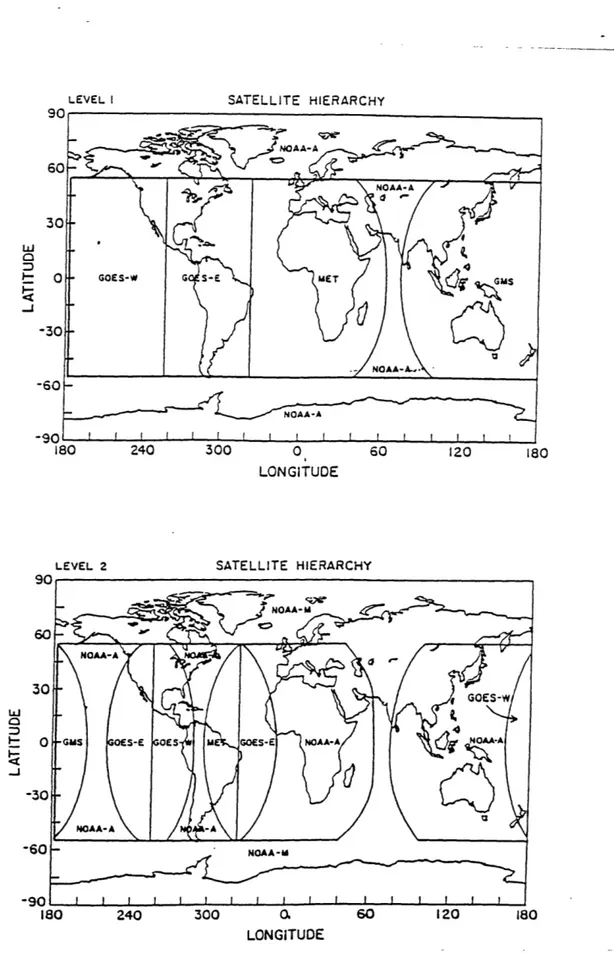
The International Satellite Cloud Climatology Project (ISCCP) was established as the first project of the World Climate Research Program (WCRP 1984) to collect and analyze satellite radiance measurements to infer the global distribution of cloud radiative properties and their diurnal and seasonal variations. Operational data collection and processing for ISCCP have been underway since July 1983. To obtain global averages while resolving diurnal variations, the project planned to use data from at least one polar-orbiting and five geostationary weather satellite.

Fig. 1-1 shows the regional coverage provided by satellites used for ISCCP.

The Satellites measured radiances in each pixel for VIS(O.6 p9m) and IR(1 lum) wavelengths which depend on ozone and water abundance. The data have been sampled to a pixel spacing of about 30Km . Hence in the cloud analysis each image pixel is treated as representing a specific scene about 30Km across. Each pixel was separated into cloudy and clear scenes. All image pixels containing

Original ISCCP plans called for reporting the properties of five cloud types ;low, middle, high, cirrus and deep convective clouds. The latter two types were qualitatively defined to be optically thin and thick high clouds, respectively. The cloud types are identified by their values of cloud top pressure and cloud optical thickness. To allow for diurnal studies and to study the effects of the cloud top adjustment procedure, the cloud top pressure distribution determined by the IR-only algorithm is also reported during the day-time along with the cloud top pressure distribution determined

by the VIS/IR algorithm but without the cloud top adjustment.

The deep convections in the tropics, in which we were interested have about 8 - 10 km height. Therefore, the highest cloud data can be the index of deep convection. In this paper, two kinds of cloud type are analyzed. The first is that with the lowest cloud top pressure (5mb < P < 180mb), which is determined by the VIS/IR algorithm. The second is that with the lowest cloud top pressure and the largest optical thickness(22.63 < TAU < 119.59). Because of the need for optical thickness these data were provided only in daytime. Fig. 1-2 shows the area for which visible data can be provided in each GMT hour.

The ISCCP retrieved detailed information about the global cloud properties every three hours throughout the month. The nominal spatial resolution is 250Km. The data was given on a longitude -latitude grid with 2.5 degrees resolution on both longitude and latitude. Thus 10368 grid cells (2.5 * 2.5 degrees longitude latitude)

cover the whole globe. Each such cell contained a certain total number of pixels. "Cloud Cover" in one grid cell for the respective cloud class is defined as follows.

Cloud Cover = Number of cloudy pixels / Total number of pixels

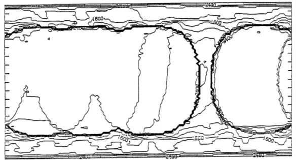
Fig. 2 shows the number of observations in a 1-year period. The 100% observation number is 2920. In this period the percent of observational coverage is at least 85% from 60N latitude to 60S latitude, except in the Indonesian Area, which is about 30%.

In this paper, the data from August 1983 to July 1987, were analyzed. Because of the Data Tape conditions, some period of the data are not included. Table 1. shows the periods which couldn't be used in this paper, and defines the seasonal means used.

In January 1985, the satellite 7 was changed to

NOAA-9. This satellite is important for the primary which used in the cloud analysis procedure. The data was calibrated to eliminate any discontinuities, to the extent possible (Rossow and Schiffer, 1991).

Table 1. 1983 0 0 0 0 0 1984 0 00 0 0 O0 0 0 O 0 0 0 0 1985 0 0 0 0 0 0 0 0 00 X 0 1986 0 0 0 0 0 0 0 2H 0 0 11H 0 1987 0 0 1H 1H 2H X 0

0: used X: unused 1H:first half used 2H: second half used

Autumn 1983(SEP,OCT,NOV) 1984(SEP,OCT,NOV) 1986(SEP,OCT,NOV)

Winter 1983(DEC)1984(JANFEB) 1984(DEC)1985(JAN,FEB)

1985(DEC)1986(JAN,FEB) 1986(DEC)1987(JAN,FEB)

Spring 1984(MAR,APR,MAY), 1985(MAR,APR,MAY) 1986(MAR,APR,MAY)

Summer 1984(JUN,JUL,AUG) 1985(JUN,JUL,AUG)

RESULT

Mean cloud cover

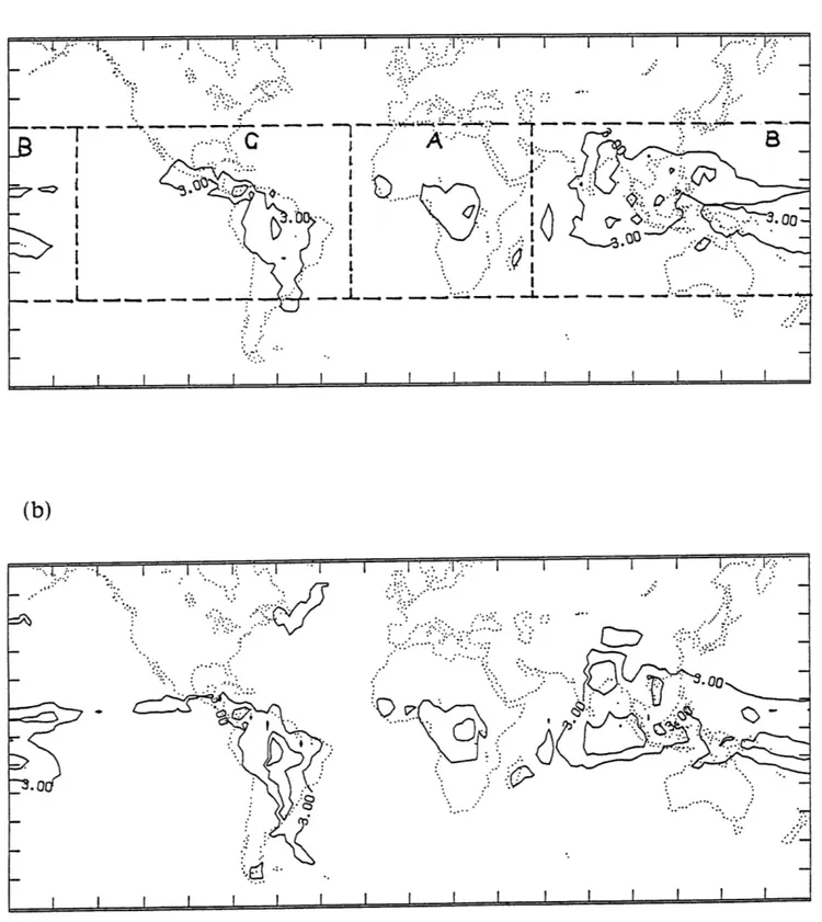
Fig 4. shows the geographical distribution of mean cloud cover

for two different period. In this map we can see 3 major convection

areas, America,especially South America, Africa and Asia with the

western equatorial Pacific.

Global diumal cycle

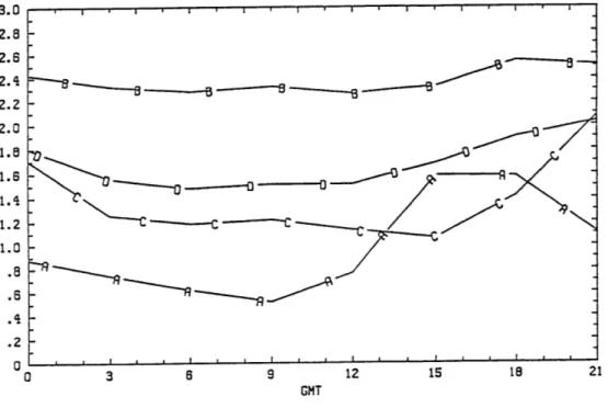
Fig 5. shows the four years average global diurnal cycle (D

line). The percent cloud coverage data were averaged from August

1983 to July 1987

in the tropics (31.25N - 31.25S) at each GMT

hour.

Also, shown for comparison, in Figure 3-1, is the carnegie

curve for the mean diurnal cycle of the global ionospheric potential.

The diurnal cycle of high cloud cover does indeed closely resemble

the diurnal cycle in Ionosphere potential, thus lending support to

Wilson's theory.

Each A,B,C line is the four year average diurnal cycle in the

respective sectors shown in Fig 4.

Because of the large amount of

cloud cover, the Asia-Austrailia sector ,B, is the major contributor

to the global deep cloud cover diurnal cycle.

Fig 6. shows the 4-year mean diurnal cycle over ocean and land.

Ocean and land are defined by whether the center of the grid cell is

located on land or on ocean from the map.

Line A is the total

tropical diurnal cycle, while lines B and C are the cycles over land

and ocean,respectively. The land cycle has a bigger amplitude, but

the ocean cycle is more similar to the total tropical cycle.

Fig 6(b)

is the same as Fig 6(a) but only the optically thick clouds, based on

the visible data, are included. Thus thick, night-time clouds are

excluded.(see Fig.1-2)

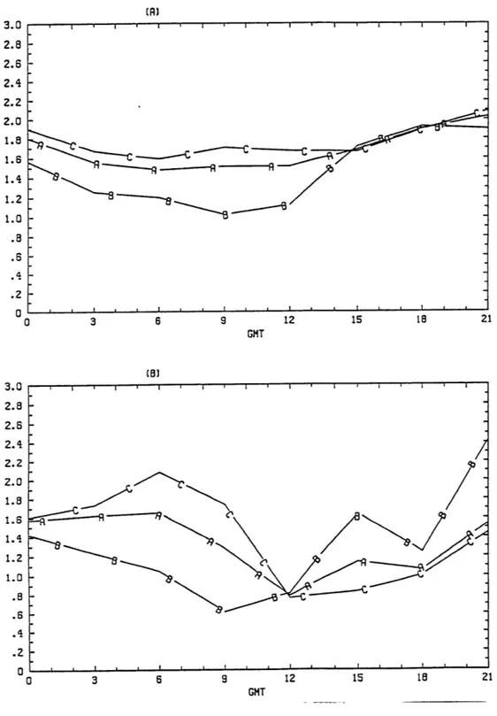
In section A, the diurnal cycle over ocean and land are very

similar. Over land, the maximum is at 15GMT which is 3-4PM in this

area. The maximum over ocean is 3 hours later than that over land.

This may be because it takes more time to heat the ocean. The

diurnal cycle amplitude of this section is very large because the

ratio of land area in this section is large,48%.

In section B, The diurnal cycle over the ocean shows two

maxima at 9 GMT and 18 GMT. In local time these are about 4-5PM

and 1-2AM. Over land, the maxima are at 6GMT and 18GMT. Because

of the three hours differences between the land and ocean, we can

suggest that the first maximum(1-2PM in the land and 4-5PM in the

ocean) is caused by diurnal heating. The second maximum(1-2AM in

both) must be caused by larger scale diurnal circulations, e.g.

Monsoon circulations.

In section C, the diurnal cycles over both land and ocean have

the same shape but different amplitudes. The maximum is at 21GMT

which is 2-3PM in the middle of this section. There is a remarkably

large diurnal cycle amplitude over land, but because 77% of this

section is ocean,there is still a big ocean contribution to the total

diurnal cycle.

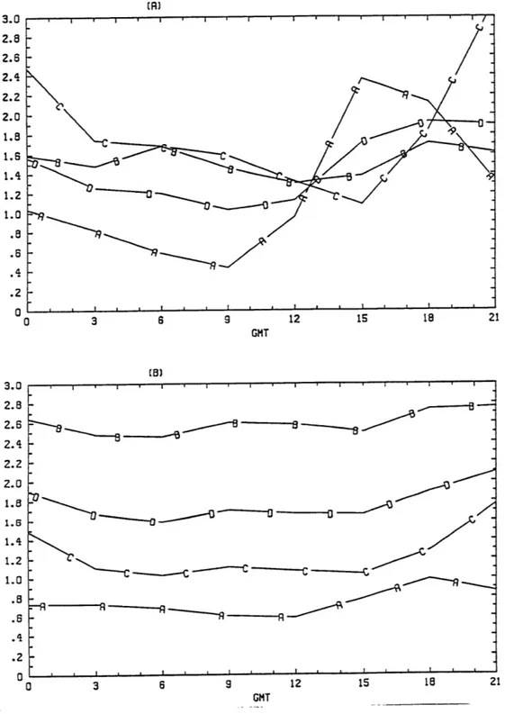
Fig 7(a). shows the diurnal cycle of the whole tropics and of

each section over land.

For comparison, Fig 3-2 is the diurnal

variation of the world's thunderstorm areas from Brook's 1925

analysis. When we compare diurnal variation of the highest clouds

with Brook's analysis, the America section(C) contributes more from

3 to 9GMT than in Brook's analysis. Thus there is no dominant

contribution of Asia and Australia, section(B). But there is a big

contribution of section B land around 6GMT, as in Brook's analysis.

Land in section A is the major contributor from 12GMT to 18GMT.

Therefore this figure is very similar to Brook's analysis, but with a

3 hour shift, and a bigger and longer contribution of the America

section. Fig 7(b). is for the ocean. The variations are very flat in all

sections.

Seasonal diurnal cycle variation

Fig 8. shows the global and sectional diurnal cycle in each

season defined in the DATA section. Line D is the diurnal cycle in

whole tropics and line A,B and C represent each section.

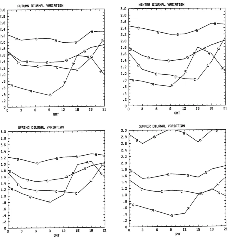
There is

not much seasonal change in diurnal cycle for the whole tropics

except in summer. But, in separate sections there are clear seasonal

differences in diurnal cycle.

The diurnal cycle in section A moves up and down seasonally

without shape changes. In this section, the major convection area is

concentrated in the southern hemisphere. Therefore, the biggest

diurnal cycle is in northern spring and winter and the smallest is in

summer. In section C, the diurnal cycle changes seasonally without

change in shape, too. But there is a big amplitude in winter and very

little in summer. In this section, more convection is located in the

southern hemisphere than the northern hemisphere as shown in Fig 4.

Therefore, there can be a bigger diurnal cycle in northern winter

when the southern part of the convection area is stronger.

We can see big differences in the summer season. This is

caused by a big change in the section B diurnal cycle and decrease in

the section A diurnal cycle. When we look at Fig 4., most of the

convection area in section B is located in the northern hemisphere.

So in the northern summer, when the ITCZ is located in northern

hemisphere, the amount of high cloud cover in section B becomes

larger. Therefore, because of the big contribution of section B, the

diurnal cycle in summer shows a 9GMT maximum as well as the

usual 21GMT maximum.

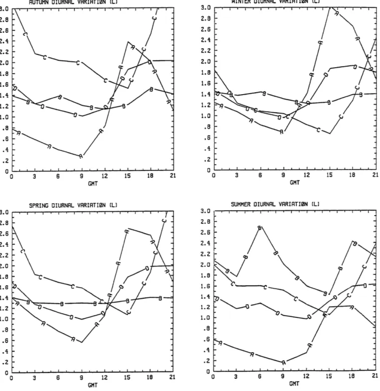
Fig 9. show the seasonal diurnal cycles over land separately. The

diurnal cycles of the whole tropical land area have big amplitudes

but there are very small seasonal changes in either amplitude or

shape except in summer.

The diurnal cycles of sections A and C have big amplitudes. And

they change seasonally but differently from each other. When we

compare these two sections, section A has the biggest diurnal cycle

in winter and small diurnal cycle in summer. But in section C, a big

diurnal cycle is shown both in spring and autumn. These two diurnal

cycles compensate each other except in summer; therefore, we can

not see any seasonal change of total diurnal cycle associated with

changes of these two sections. Section B is very flat and has not

much change except in summer.

In autumn and spring, section C is the major contributor

except around 15GMT when the section A is the major contributor.

In winter, the major contributor is section A from 12GMT to 18GMT

and section B from 3GMT to 9GMT and section C from 18GMT to 3GMT.

This is very similar to Brook's(1925) analysis. In summer, section B

is the major contributor all the time.

There are unusual changes in summer. Especially, in section B

there is a big oscillation, associated with the Monsoon period. There

are two maxima which are 6GMT and 18GMT. These are about 1-4PM

and 1-4AM in that section. There is also a prominent decrease of the

Over ocean(Fig 10.), all of the diurnal cycles are very flat

compared to over land. There are still seasonal changes in the

diurnal cycles. Section B is the major contributor to the tropical

ocean diurnal cycle in all the seasons. In spring and summer, there

are big changes in the convection in section B.

The diurnal cycles of the separate sections are anti-correlated

with each other. Therefore, even though there are big changes in

diurnal cycles in individual sections, the total diurnal cycle is not

changed as much as that of each section.

Time series (monthly)

The mean, amplitude and standard deviation of each month's

diurnal cycle were calculated for the period of August 1983 to

February 1987.

November 1985, the missing month, is interpolated

from October and December. The mean is the average of the eight 3

hourly values in the diurnal cycle of each month.

The amplitude of

the diurnal cycle is defined by the difference between the maximum

and minimum in that diurnal cycle. The standard deviation is

calculated from the eight 3 hour mean data in each month. If the

diurnal cycle is complex, this will gives a letter measure of the

daily variation.

Fig 11. shows the mean, amplitude and standard deviation of

diurnal cycle for the whole tropical area(31.25N - 31.25S).

In the

mean data there is a jump at February 1985. It may be caused by the

satellite change described in DATA section. The amplitude may have

an annual cycle e.g., the minimum seems to occur every 12 months.

The standard deviation data is highly correlated with the amplitude

data. This means that most of the diurnal cycles have one maximum

and one minimum.

Fig 12. shows the same data but over land and ocean

separately. Over land there is a annual cycle in amplitude and mean.

They are very well correlated.

The maxima occur in October and

March and the minimum in July. Thus the high clouds over land are

well developed mostly in the transition seasons.

Over ocean, the variations in the diurnal cycle amplitude are

smaller than over land, and it is difficult to see any cycles in the

ocean data. These time series are more similar to the total, i.e., the

monthly change of the global diurnal cycle is dominated by ocean

areas.

Fig 13. shows the same data but for each section. In section A,

the annual cycle in the mean is more prominent. The amplitude of the

diurnal cycle also has an annual cycle which is well matched with

the mean's cycle. The maxima are in the southern winter season.

In section B, the mean of the diurnal cycle is very large, i.e,

this section is the biggest convection area. But the amplitude of the

diurnal cycle is very small compared to the other sections.

And

there is a big jump of mean near February 1985. This time is the

period when the NOAA satellite is changed, and that satellite covers

this B section. This circumstance may affect the cloud cover data in

this section. Unusually big amplitudes occurred from June 1984 to

September 1984.

In section

C,

there are bigger annual changes in the diurnal

cycle amplitudes.

The biggest amplitudes of diurnal cycle occur in

February and March. The mean data have a no obvious cycle.

In each sector AB and C, the same analyses are done for land

and ocean separately.(see Fig 14) In section A, land and ocean both

have a clear annual cycle. And both have March and April maxima.

However their minima are in June or July over land, but in January

over ocean. Therefore, land and ocean have different annual cycles

but both with maxima in March.

In section B(Fig.15), the land data has a clear annual cycle

with an August maximum and January or February minimum.

Therefore, it is clear that there is a strong association with the

monsoon. The amplitude data are very similar to the mean data. The

ocean shows very little annual cycle. An unusual peak is seen in

summer 1984, especially over land but also over ocean. In January

1983, there was a very strong El Nino.

This meant anomalous

heating in the Pacific. This type of event take a year or two to

re-equilibriate. This may have affected this period.

Over the ocean in sector C,(Fig.16) we cannot see any specific

cycle in the mean data, but, in amplitude there is a clear annual

cycle with a maximum in June. Over land, there is a half year period

cycle in both amplitude and mean data, with maxima in August and

February. In this sector, there are land areas in both hemispheres so

that, as the ITCZ moves from one hemisphere to the other, the

convection over land is well developed twice each year. Therefore,

in winter and summer, when ITCZ is located over land, the diurnal

cycle of cloud cover becomes larger.

In the C sector over land the cycles in the mean and amplitude

are bigger than those over ocean. But still there is a nonnegligible

annual cycle in the diurnal cycle amplitude over ocean, and because

of the larger area of ocean than land, the contribution of ocean to

total diurnal cycle becomes important. Actually the annual cycle in

the total convection in sector C is dominated by the annual cycle

over the oceans.

Correlation

Table 2. shows correlation coefficients of the time series for

different areas.

The mean of diurnal cycle for the whole tropics is most

correlated with section B, but the amplitude of the diurnal cycle is

the whole tropics land diurnal cycle section is the diurnal cycle of

America (section C). Over ocean, the diurnal cycle of section B is

most correlated with total ocean diurnal cycle.

In each section, the diurnal cycle of ocean and land are not

much correlated.

AREA MEAN AMPLITUDE Total Section A 30.1 56.5 Total Section B 80.1 59.5 Total Section C 60.7 63.7 Total LAND 60.9 63.6 Total OCEAN 96.2 84.3 LAND OCEAN 37.3 23.7 Section A : Section B -18.7 Section A : Section C 34.8 Section B : Section C 11.5 LAND Section A : Section B -30.7 -48.0 Section A : Section C - 3.2 48.2 Section B Section C - 1.3 -31.8

Land Total Section A 58.7 73.3

Land Total Section B 20.3 -10.7

Land Total Section C 63.6 72.2

OCEAN

Section A Section B 3.1 19.5

Section A Section C 3.8 -65.0

Section B Section C -12.6 -19.8

Ocean Total : Section A 24.1 8.0

Ocean Total : Section B 64.8 68.3

Ocean Total : Section C 53.2 44.3

SECTION A LAND OCEAN 0.4 -50.9 SECTION B LAND OCEAN 20.4 63.1 SECTION A LAND OCEAN 38.5 11.4

CONCLUSION

1) In tropics there are three major convection areas which are

America, especially South America, Africa and Asia with the

western equatorial Pacific.

2) The Diurnal cycle of high cloud cover closely resemble the

diurnal cycle in Ionosphere potential, thus lending support the

Wilson's theory.

3)

Asia-Austrailia region is the major contributor to the global

deep cloud cover diurnal cycle.

4) The diurnal cycle of the deep cloud cover over land is similar to

the world's thunderstorm area analysis by Brooks, but with a 3 hour

shift , and a bigger and longer contribution of the America section.

5) In each sections there are clear seasonal differences in diurnal

cycle. But, the seasonal changes of the diurnal cycle of the separate

sections are anti-correlated with each other.

Therefore, even

though there is a big seasonal change in diurnal cycle in individual

sections, the total diurnal cycle is not changed as much as that of

each section.

But, summer season shows very different diurnal cycle.

6) The monthly mean and amplitude of the diurnal cycle over the

land shows a very clear annual cycle.

The maxima occur in October

and March and minimum in July.

7) In each section, there are more clear annual cycle. In section A,

land and ocean both have a clear annual cycle, and both have March

and April maxima. However, their minima are in June or July over

land, but in January over ocean. In section B, the land data has a

clear annual cycle with an August maximum and January or February

minimum.

In section C, the land data has a half year cycle with

maxima in August and February.

8)

The mean of diurnal cycle for the whole tropics is most

correlated with section B, but the amplitude of the diurnal cycle is

SATELLITE HIERARCHY -90 L-180 LEVEL 2 240 300 0 60 120 LONGITUDE 180 SATELLITE HIERARCHY LO LONGITUDE

Fig 1-1

Regional coverage provided by satellites used for ISCCP:

Level 1 of hierarchy indicates the preferred satellite for eacr

location while Level 2 indicates the second choice used if the

preferred satellite is not available.

3'.,~ *'. I ,..t, 4 .f *~ ~1' I' S. ~,f *?~\ ~ -J-WWWLWJJ I I I' I-I-i -, 'V L k, I A ff I

83 AUG - 84 JUL (3HR INTERVAL OBS)

84 AUG - 85 JUL (3HR INTERVAL OBS)

Fig.

2

_{Number of observation in each one year period (a) August 1983 to}

July 984. (b) August 1984 through July 1985. e.g., 2920 will be the complete

120 110 100

I

I

I

I

...i,...f...,.

GMT

Fig. 3-1 Carnegie curve obtained from the average of electric field

measurements made by the Carnegie research vessel during

ocean cruises during the 1920's. (After Chalmers, 1957.)

A place Is regarded as hAving been in a thunder area at a

specified time if thunder was audble in the intem.al fren 120 60m before to 60m after that time.Th ok N 100 ~~ ~ -00 e 40 2 4 6 8 10 12 14 15 18 20 20 GM]

Fig. 3-2 Universal diurnal variation of global electrical circuit and

its control by three major zones of convection.

(a)

C

7

-A

S

(b)

Fig. 4

Mean high cloud (5mb

-

180mb cloud top pressure) fraction

coverage.(%) (a) August 1983 thru January 1985. (b) February

1985 thru July 1987. Contour intervals are 3%.

32

I I

3.0 2.8 2.6 2.4 a ----2.2 2.0 1.4 1.2 C C 1.0 .8 .2-0 3 6 9 12 15 18 21 GMT

Fig. 5 High cloud diurnal cycle following universal time (August 1983

thru July 1987).

X axis is GMT time. Y axis is cloud fraction

coverage(%).

Line D is the for total tropics(31.25N-31.25S). Line AB and C are for

section A,B and C.

(R) 3.0 2.8 2.6 2.4 2.2 2.0 1.5 1.4 1.2 1.0 .8 .6 .4 .2 0 0 3 6 9 12 15 18 21 GMT (B3 2.8 2.6 2.4 2.2 2.0 1.8 1.6 1.4 .2 .o -0 0 3 6 9 12 15 18 21 GMT

Fig. 6

High cloud diurnal cycle following universal time. Line A is

the total for each area, B is for land and C is for ocean. (a)

Tropics (b) Tropics but for VIS data only (c) Section A (d)

Section B (e) Section C

3.0 2.8 2.5 2.4 2. Z 2.0 1.8 1.6 1.4 1.2 1.0 .8 .5 .4 .2 0 3.0 2.8 2.6 2.4 2. Z 2.0 1.8 1.5 1.4 1.2 1.0 .8 .5 .4 .2 0 3 6 9 12 15 18 ---

-3.0 2.8 2.6 2.4 2.2 2.0 1. -1.6 1.4 1.2 1.0 .8 .6 .4 .2 0 0

36

2.8 2.6 2.4 2.2 2.0 1.8 -1.6 1.4 .2 -0 0 3 8 9 12 15 is 21 GMT .0 2.6 1.4 1.2 1.0 3.8 2.5 2.2 1.2 1.0 .2 0 0 3 6 9 12 15 18 21 GMT

Fig. 7 High cloud diurnal cycle following universal time

over land

and ocean separately. Line A, B and C are for section A, B

and C respectively. Line D is for total. (a) land (b) ocean

RUTUMN DIURNAL VARIATION

I I I

0 3 6 9 12 15 18 21

GMT

WINTER DIURNAL VARIATION

3.0 iillII I I I 2.8 2.6 2.4 2.2 2.0 1.8 1.6 1.4 .2 0 0 3 6 9 12 15 18 21

SPRING DIURNAL VARIRTION

3.0 2.8 2.6 2.4 2. 2 2.0 1.8 1.6 1.4 1.2 1.0 .8 .6 .4 .2 0 3 6 9 12 15 18 21 GMT

SUMMER DIURNAL VRRIRTION

0 3 6 9 12 15 16 21 GMT

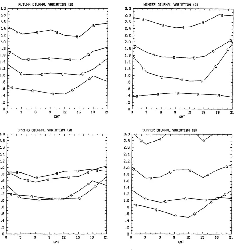
Fig. 8 Seasonal high cloud diurnal cycle. Line A, B and C are for section

A, B and C respectively. Line D is for total. (Each season defined in

DATA section)

38

3.0 2.8 2.8 2.4 2.2 2.0 1.8 1.6 1.4 1.2 1.0 .8 .6 .4 .2 0 3.0 2.8 2.6 2.4 2.2 2.0 1.8 1.6 1.4 1.2 1.0 .8 .6 .4 0

AUTUMN DIURNAL VARIATION EL)

0 3 6 9 12 15 18 21

SPRING DIURNAL VARIATION IL]

0 3 6 9 12 15 18 21

GMT

WINTER DIURNAL VARIATION (L) 2.8 --2.6 2.4 2.2 2.0 1.6 1.4 1.2 1.0 -8- .6-.2 0 0 3 6 9 12 15 18 21

SUMMER DIURNAL VARIATION [LI

0 3 6 9 12 15 18 21

GMT

AUTUMN DIURNAL VARIATION (03

-- 0

-- - -- -C

0 3 6 9 12 15 18 21 GMT

SPRING DIURNAL VARIATION (0)

0 3 6 9 12 15 18 21

Fig. 10 Same as Fig 8 except

WINTER DIURNAL VARIATION (0)

3.0 Il I I II . 2.8 2.6 2.4 2.2 2.0 1.8 1.4 1.2 -1.0 .8 .6 --.2 0 0 3 6 9 12 15 18 21 3.0 2.8 2.6 2.4 2.2 2.0 1.8 1.6 1.4 1.2 1.0 .6 .6 .4 .2 0

SUMMER DIURNAL VARIATION (0)

3 3 6 9 12 15 18 21

GMT

for ocean only.

40

TOTRL

-3.5

3.0

2.5

.5

Fig. 11 Monthly changes of diurnal cycle (From August 1983 to February

1987). Line M is the mean, A is ampitude of diurnal cycle and D is

standard deviation for diurnal cycle.

(a)

LRND

2.5

.5

Fig. 12 Same as Fig 11 except for land and ocean seperately. (a) land

(b) ocean

(b)

OCERN

0

(a)

SECTION

R

3.5

3.0

.5

Fig. 13 Same as Fig 11 except for each section. (a) section A (b) section B

(c) section C

44

(b)

SECTION B

0

(c)

SECTION C

46

(a)

SECTION

R

(LRNU)

A

3.5

3.0

.5

Fig. 14 Same as Fig 11 except for land and ocean seperately in section A.

(a) land

(b) ocean

12 24 36 4;

---(b)

SECTION

R

(OCERN)

A

48

3.0

Fig. 15 Same as Fig 14 except for section B

(a) land

(b) ocean

(b) SECTION B (OCERN)

50

(a)

SECTION C (LRNU)

3.5

Fig. 16 Same as Fig 14 except for section C

(a) land

(b) ocean

(b) SECTION C (OCERN)

3.5

52

Reference

Albright Mark D, Ernest E. Recker and Richard J Reed, 1985: The

Diurnal Variation of Deep Convection and Inferred

Precipitation in the Central Tropical Pacific During

January-February 1979 .Mon. Wea. Rev., 113, 1663-1680

Brooks, C. E. P., 1925. Geophys. Mem.(Air Ministry, Meteor. Office) 24 : 147-164

Chalmers, J. A., 1957. Atmospheric Electricity, London: Pergamon. Gish, O.H., and G. R. Wait, 1950. J. Geophys. Res. 55 : 473-484. Hoskins, B., and D. Karoly, 1981: The steady linear response of a

spherical atmosphere to thermal and prographic forcing. J. Atmos. Sci., 38, 1179-1196

Mauchly, S. J., 1923. Terr. Mag. Atmos. Elect. 28:61-81

Reed Richard J. and Kenneth D. Jaffe, 1981: Diurnal Variation of

Summer Convection Over West Africa and the Tropical

Eastern Atlantic During 1974 and 1978. Mon. Wea

Rev. ,109,2527-2534

Richards, F. and P. Arkin, 1981: On the relationships between

satellite-observed clud cover and precipitation. Mon.

Wea. Rev., 109, 1081-1093

Rossow William B. and Robert A. Schiffer, 1990: ISCCP Cloud Data

Product. AMS, Vol 72, No. 1, Jan. 1991

Trent, E. M., and S. G. Gathman, 1972. Pure Appl. Geophys. 100:60-69 Wexler Raymond, 1983:Relative Frequancy and Diurnal Variation of

High Cold Clouds in the Tropical Atlantic Pacific. Mon.

Wea. Rev., 111,1300- 1304

Whipple, F. J. W., 1929.

Quart.