Past and present of sediment and carbon biogeochemical cycling models

(1)

HAL Id: hal-00297727

https://hal.archives-ouvertes.fr/hal-00297727

Submitted on 24 May 2004

HAL is a multi-disciplinary open access

archive for the deposit and dissemination of sci-entific research documents, whether they are pub-lished or not. The documents may come from teaching and research institutions in France or abroad, or from public or private research centers.

L’archive ouverte pluridisciplinaire HAL, est destinée au dépôt et à la diffusion de documents scientifiques de niveau recherche, publiés ou non, émanant des établissements d’enseignement et de recherche français ou étrangers, des laboratoires publics ou privés.

Past and present of sediment and carbon biogeochemical

cycling models

F. T. Mackenzie, A. Lerman, A. J. Andersson

To cite this version:

F. T. Mackenzie, A. Lerman, A. J. Andersson. Past and present of sediment and carbon biogeochemical cycling models. Biogeosciences Discussions, European Geosciences Union, 2004, 1 (1), pp.27-85. �hal-00297727�

(2)

BGD

1, 27–85, 2004

Carbon cycle models

F. T. Mackenzie et al. Title Page Abstract Introduction Conclusions References Tables Figures J I J I Back Close

Full Screen / Esc

Print Version Interactive Discussion © EGU 2004 Biogeosciences Discussions, 1, 27–85, 2004 www.biogeosciences.net/bgd/1/27/ SRef-ID: 1810-6285/bgd/2004-1-27 © European Geosciences Union 2004

Biogeosciences Discussions

Biogeosciences Discussions is the access reviewed discussion forum of Biogeosciences

Past and present of sediment and carbon

biogeochemical cycling models

F. T. Mackenzie1, A. Lerman2, and A. J. Andersson1 1

Department of Oceanography, University of Hawaii, Honolulu, Hawaii 96822, USA

2

Department of Geological Sciences, Northwestern University, Evanston, Illinois 60208, USA Received: 25 April 2004 – Accepted: 18 May 2004 – Published: 24 May 2004

(3)

BGD

1, 27–85, 2004

Full Screen / Esc

Print Version

Interactive Discussion

The global carbon cycle is part of the much more extensive sedimentary cycle that involves large masses of carbon in the Earth’s inner and outer spheres. Studies of the carbon cycle generally followed a progression in knowledge of the natural biolog-ical, then chembiolog-ical, and finally geological processes involved, culminating in a more 5

or less integrated picture of the biogeochemical carbon cycle by the 1920s. However, knowledge of the ocean’s carbon cycle behavior has only within the last few decades progressed to a stage where meaningful discussion of carbon processes on an annual to millennial time scale can take place. In geologically older and pre-industrial time, the ocean was generally a net source of CO₂ emissions to the atmosphere owing to the 10

mineralization of land-derived organic matter in addition to that produced in situ and to the process of CaCO₃precipitation. Due to rising atmospheric CO₂concentrations be-cause of fossil fuel combustion and land use changes, the direction of the air-sea CO₂ flux has reversed, leading to the ocean as a whole being a net sink of anthropogenic CO₂. The present thickness of the surface ocean layer, where part of the anthropogenic 15

CO₂ emissions are stored, is estimated as of the order of a few hundred meters. The oceanic coastal zone net air-sea CO₂exchange flux has also probably changed during industrial time. Model projections indicate that in pre-industrial times, the coastal zone may have been net heterotrophic, releasing CO₂ to the atmosphere from the imbal-ance between gross photosynthesis and total respiration. This, coupled with extensive 20

CaCO₃ precipitation in coastal zone environments, led to a net flux of CO₂ out of the system. During industrial time the coastal zone ocean has tended to reverse its trophic status toward a non-steady state situation of net autotrophy, resulting in net uptake of anthropogenic CO₂and storage of carbon in the coastal ocean, despite the significant calcification that still occurs in this region. Furthermore, evidence from the inorganic 25

carbon cycle indicates that deposition and net storage of CaCO₃in sediments exceed inflow of inorganic carbon from land and produce CO₂emissions to the atmosphere. In the shallow-water coastal zone, increase in atmospheric CO₂during the last 300 years

(4)

BGD

1, 27–85, 2004

Full Screen / Esc

Print Version

of industrial time may have reduced the rate of calcification, and continuation of this trend is an issue of serious environmental concern in the global carbon balance.

1. Introduction

Our understanding of the behavior of carbon in nature, as the main chemical con-stituent of life on Earth, has progressed through observations and modeling of the 5

short-term processes of formation and decay of living organic matter by the land and oceanic biotas, the somewhat longer processes of carbon cycling in the oceans, and the geologically much longer time scales of the sedimentary cycle that involves deposi-tion of sediments on the ocean floor and their subsequent migradeposi-tion to the mantle and reincorporation in the continental mass.

10

In the early 1970s, Garrels and Mackenzie (1972) published a model describing the steady state cycling of eleven elements involved in the formation and destruction of sedimentary rocks: Al, C, Ca, Cl, Fe, K, Mg, Na, S, Si, and Ti. To our knowledge, this was the first modern attempt to model comprehensively and interactively the biogeo-chemical cycles of the major elements in the ocean-atmosphere-sediment system. The 15

model, incorporating much of the basic thinking advanced in “Evolution of Sedimentary Rocks” (Garrels and Mackenzie, 1971), derived a steady state mass balance for the sedimentary system consistent with the observed composition of the atmosphere, bio-sphere, ocean, stream and groundwater reservoirs, as well as the ages and average composition of sedimentary rocks. Of importance to the present paper with respect 20

to the carbon balance were the conclusions from the Garrels and Mackenzie model that on the geologic time scale (1) the global oceans are generally a net heterotrophic system, with the sum of aerobic and anaerobic respiration exceeding the gross pro-duction of organic matter in the ocean and hence are a source of CO₂, reflecting the imbalance in the fluxes related to these processes, and (2) the oceans must act as a 25

source of CO₂ to the atmosphere from the processes of carbonate precipitation and accumulation.

(5)

BGD

1, 27–85, 2004

Full Screen / Esc

Print Version

In this paper we explore some of the more recent developments related to these conclusions in the context of the history of modeling of the carbon cycle, and what models tell us about the pre-industrial to future air-sea transfers of CO₂in the shallow-ocean environment.

2. History of modeling concepts of the carbon cycle 5

Perceptions of many natural processes as cycles are undoubtedly rooted in the changes of day and night, seasons of the year, and astronomical observations in ancient times, from which the concept of cycles and epicycles of planetary motions emerged. Another cyclical phenomenon of great importance, but less obvious to the eye, is the cycle of water on Earth that is also responsible for the circulation and trans-10

port of many materials near and at the Earth surface. An early description of the water cycle is sometimes attributed to a verse in the book of “Ecclesiastes” (i, 7), believed to have been written in the 3rd century B.C., that speaks of the rivers running into the sea and returning from there to their place of origin (but there is no mention of the salt nor of water evaporation and precipitation). The modern concept of the global water 15

cycle is the result of observations of atmospheric precipitation, its infiltration into the ground, river runoff, and experiments on water evaporation conducted in the 1600s in France and England (Linsey, 1964). These concepts were well accepted by the time of the first edition of Charles Lyell’s “Principles of Geology” (Lyell, 1830). By 1872, Lyell referred to a cycle – “the whole cycle of changes returns into itself” – in his description 20

of alternating generations of asexual and sexual reproduction among certain classes of marine invertebrates, which he likened to metamorphosis in insects (Lyell, 1872, 1875).

As to geochemical cycles, an early treatment of the subject appeared in 1875, where several chapters on the cycles of chemical elements were included in a book on Earth 25

history by F. Mohr, a professor at the University of Bonn, with chapters on the silicon and carbon cycles among them (Mohr, 1875). Since then and to the early part of the

(6)

BGD

1, 27–85, 2004

Full Screen / Esc

Print Version

20th century, the cyclical nature of the major geological processes, that involve shaping of the Earth surface by tectonic forces and running water, and transfer of molten rock material from depth to the surface, developed into a well accepted concept.

The earlier discoveries that plants use carbon dioxide for growth in sunlight and return it to the atmosphere in darkness must have been the first scientific observations 5

of one important part of the carbon cycle. A step further in the carbon cycle was that living plants use carbon dioxide to make their tissues, and when they die they become organic matter in soil that decomposes to carbon dioxide. The formation of organic matter from carbon dioxide and water under the action of light, the process known as photosynthesis, has been studied since the later part of the 1700s, when molecular 10

oxygen was discovered in the process and carbon dioxide identified as a component of air. Short histories of successive discoveries in photosynthesis, since the late 1700s to the 20th century, have been given by several authors (Gaffron, 1964; Meyer, 1964; Bassham, 1974; Whitmarsh and Govindjee, 1995). Presentation of the first general scheme of the carbon and nitrogen cycles has been attributed to the French chemist, 15

J. B. A. Dumas, in 1841 (Rankama and Sahama, 1950).

By the early 20th century, concepts of the cycles of the biologically important ele-ments began to recognize their interactions and expanded to include the various phys-ical, chemphys-ical, geologphys-ical, and biological processes on Earth, and the material flows between living organisms and their surroundings, as well as between different environ-20

mental reservoirs. In the 1920s, the cycles of the chemical elements that are involved in biological processes – carbon, nitrogen, and phosphorus – and are also transported between soil, crustal rocks, atmosphere, land, and ocean waters, and the Earth’s inte-rior were sufficiently well recognized. Alfred Lotka wrote in his book “Elements of Phys-ical Biology”, published in 1925, chapters on the cycles of carbon dioxide, nitrogen, and 25

phosphorus that present a modern treatment of what we call today the biogeochemi-cal cycles (Lotka, 1925). Furthermore, he wrote that his ideas of the nutrient element cycles and mathematical treatment of biogeochemical problems were developed as far back as 1902 and in his publications starting in 1907. The term biogeochemical

(7)

BGD

1, 27–85, 2004

Full Screen / Esc

Print Version

reflects the fact that biological, physical, and chemical processes play important roles and interact with each other in the element cycles that are mediated by photosynthetic primary production and respiration or mineralization of organic matter.

By 1950, the geochemical cycles of elements in the Earth interior and on its surface became textbook material (Rankama and Sahama, 1950), having a variable degree 5

of detail for each cycle that reflected the uneven knowledge of igneous and sedimen-tary reservoirs and some of the inter-reservoir fluxes at the time. This early, if not first, systematic textbook treatment of the geochemical cycles presented diagrams of the geochemical reservoirs as boxes and fluxes between them, and tabulations of the elemental concentrations or masses in some of the individual reservoirs. Also, plant 10

and animal ecosystems began to be represented as models of a varying degree of de-tail based on systems of reservoirs (ecosystem components) and inter-reservoir fluxes (transfers of material or energy) (e.g. Odum, 1983). Subsequent decades produced the knowledge we have today of the chemical speciation of the elements in the different compartments of the Earth, their abundances, and mechanisms responsible for their 15

flows. While the earlier models of the global biogeochemical cycles of individual ele-ments were static, describing the cycles without their evolution in time, developele-ments in the mathematical treatment of time-dependent multireservoir systems (e.g. Meadows et al., 1972) found their application in the analysis of geochemical cycles (e.g. Lerman et al., 1975). Since then, there has been a great proliferation of cycle models, and 20

in particular of carbon cycle models, at very different physical and time scales, aimed at interpretation of cycle evolution in the past and its projection into the future for the world as a whole, as well as for such global reservoirs as the atmosphere, land, coastal oceanic zone, and the open ocean.

Considerable attention has been focused on the global sedimentary cycle and the 25

cycling of salts in the ocean as a result of Kelvin’s (William Thomson, later Lord Kelvin) estimates of the age of the Earth between 24 and 94 Ma, made between 1864 and 1899 (Carslaw and Jaeger, 1959), and the estimates of the age of the ocean from the rate of accumulation of sodium brought in by rivers, as was done, for example, by Joly

(8)

BGD

1, 27–85, 2004

Full Screen / Esc

Print Version

(1899) whose estimated age of the ocean was about 90 Ma. Recognition of the impor-tance of crustal denudation and sediment transport as ongoing geological processes on a global scale is attributed to James Hutton (1726-1797). Gregor (1988, 1992) summarized and discussed in detail the geological arguments in the second half of the 1800s and the early 1900s for the recycling of oceanic sediments after their deposition 5

(Croll, 1871) and for the existing sinks of dissolved salts in ocean water, such as their removal by adsorption on clays, entrapment in sediment pore water, and formation of evaporites, all of which were contrary to the idea of the ocean continuously filling up with dissolved salts (Hunt, 1875; Fisher, 1900; Becker, 1910). Garrels and Mackenzie (1971) presented the concepts of the sedimentary cycling of materials, that had laid 10

dormant for some years, in book form, and in 1972 these two authors developed a quantitative model of the complete sedimentary rock cycle. Quantitative estimates of sediment recycling rates, based on mass-age sediment distributions, have been made by Gregor (1970, 1980) and Garrels and Mackenzie (1971, 1972): the total sedimen-tary mass has a mass half-age of 600 Ma. The differential weathering rates of different 15

rock types gave the half-age of shales and sandstones of about 600 Ma, longer than the ages of more easily weathered rocks, such as carbonates of half-age 300 Ma and evaporites of about 200 Ma. Later work (Veizer, 1988) showed that the recycling rates of the sedimentary lithosphere and the various rock types within it are mainly a func-tion of the recycling rates of the tectonic realms, such as active margin basins, oceanic 20

crust, and continental basement, in which the sediments were accumulated.

3. Carbon cycle in the Earth interior and on the surface

Geochemical cycles involving the interior of the Earth are known as endogenic cy-cles, and they are generally characterized by long time scales of the orders of 108 to 109 years. The sediments, hydrosphere, biosphere, and atmosphere are grouped in 25

the exogenic cycle, and a few authors define the exogenic cycle as the reservoirs of the biosphere, hydrosphere, and atmosphere, relegating the sediments to the

(9)

endo-BGD

1, 27–85, 2004

Full Screen / Esc

Print Version

genic cycle. A summary of the carbon content of the major endogenic and exogenic reservoirs is given in Table 1. Among the endogenic reservoirs, the upper mantle is the largest reservoir of carbon and its carbon content exceeds that of all the exogenic reservoirs. On the Earth surface, the sediments are by far the largest carbon reser-voir containing carbonate sediments and rocks, mostly calcite and dolomite, and or-5

ganic matter. The mass of carbon in known fossil fuel reserves (different types of coal, petroleum, and hydrocarbon gases) amounts to a very small fraction, less than 0.5%, of sedimentary organic carbon. The ocean contains about 50 times as much carbon as the present-day atmosphere, which makes it an important reservoir for exchange with atmospheric CO₂ under changing environmental conditions that may affect the CO₂ 10

solubility in ocean water. Land plants contain a mass of carbon comparable to that of the atmosphere, and the two carbon reservoirs would have been nearly of equal mass in pre-industrial time when atmospheric CO₂ stood at 280 ppmv. The similar masses of carbon in land plants and the atmosphere suggest that rapid and strong changes in land vegetation cover, such as due to extensive fires or epidemic mortality, might be 15

rapidly reflected in a rise of atmospheric CO₂. Although the carbon mass in oceanic primary producers amounts to 1/200 of land plants, the roles of the two biotas in the fix-ation of carbon by primary production are comparable: net primary production on land is 60×109ton C/yr (5250×1012mol/yr), as compared with 37 to 45×109ton C/yr (3100 to 3750×1012 mol/yr) in the ocean, resulting in a much shorter turnover or residence 20

time of carbon in oceanic biota (e.g. Schlesinger, 1997; Mackenzie, 2003).

3.1. The global rock cycle

The carbon cycle is part of the much bigger rock cycle that includes deeper as well as the outer Earth shells. The rock cycle is a conceptual model of material transfers between the Earth interior and its surface or, more specifically, between the mantle, 25

crystalline crust, sedimentary rocks, and younger unconsolidated sediments. A model of the rock cycle that shows the essentials of sediment formation and recycling is given in Fig. 1. Sediments are formed mainly by erosion of crustal rocks (flux S_c), and they

(10)

BGD

1, 27–85, 2004

Full Screen / Esc

Print Version

are recycled by erosion, redeposition, and continental accretion (flux S_s). Sediments are returned to the crystalline crust by metamorphism (flux C_s) and to the upper mantle by subduction of the ocean floor. The more recent estimates of the masses of sedi-ments, continental and oceanic crust, and upper mantle differ somewhat from those used by Gregor (1988), as shown in italics for the reservoirs in Fig. 1, but they do not 5

affect the conceptual nature of the rock cycle and its fluxes. Although neither the water reservoirs nor flows are shown in the rock cycle of Fig. 1, they are implicit in the dia-gram as the main transport agents that are responsible for the chemically reactive and physical material flows within the system.

The sediment recycling rate, S_s=7×109ton yr−1, and the sediment mass of 3×1018 10

ton give the sediment mean age of 3×1018/7×109≈430×106 yr. Because old recy-cled sediments are redeposited as new sediments, a total global sedimentation rate is S_s+S_c=9×109 ton yr−1. It is instructive to compare this rate with other flux esti-mates. Global sedimentation in the oceans includes among others the following major contributions:

15

1. transport of dissolved materials by rivers and surface runoff to the oceans; 2. riverine transport of particulate materials from land;

3. sedimentation and burial of biogenic (mostly CaCO₃, SiO₂ and organic carbon taken as CH₂O) and inorganic mineral phases forming in ocean water and in ocean-floor sediments;

20

4. wind-transported dust; and 5. glacial ice-derived debris.

Rivers transport to the oceans between 2.78 and 4.43×109 ton yr−1 of dissolved materials derived from the chemical weathering of crystalline and sedimentary rocks (Garrels and Mackenzie, 1971; Drever, 1988; Berner and Berner, 1996). An estimated 25

(11)

BGD

1, 27–85, 2004

Full Screen / Esc

Print Version

20, and 20×109 ton yr−1 (Garrels and Mackenzie, 1971; Holland, 1978; Milliman and Syvitski, 1992; Berner and Berner, 1996). The suspended particle inflow is distributed unevenly over the ocean floor, where a major part of the input is deposited in the con-tinental margins (about 80%). The wind-blown dust deposition on the ocean has been variably estimated as 1.1±0.5×109ton yr−1(Goldberg, 1971), 0.06×109ton yr−1 (Gar-5

rels and Mackenzie, 1971), and global eolian dust deposition of 0.53 to 0.85×109 ton yr−1 (Prospero, 1981; Rea et al., 1994). Additionally, about 2×109 ton yr−1 enter the ocean as glacial ice debris (Garrels and Mackenzie, 1971). Present-day accumulation rates of CaCO₃ and SiO₂ on the sea floor amount to 3.2×109 ton yr−1 and 0.4×109 ton yr−1, respectively. The organic matter accumulation rate as CH₂O is 0.5 ton yr−1. 10

Thus these fluxes account for about 26×109 ton yr−1 of materials accumulating in the oceans; that is, more than the average accumulation rate of about 10×109ton yr−1 for the past 1000 years (Wollast and Mackenzie, 1983; Chester, 2000). This shows that the ocean is not in steady state on the millennial time scale with respect to inputs and outputs of materials. In addition, the present rate of accumulation of solid sediments in 15

the ocean by the five agents listed above is about three times higher than the average geologic rate of transfer (Garrels and Mackenzie, 1972; Garrels and Perry, 1974), prob-ably reflecting the influence of relatively high continents of the present, the Pleistocene glaciation, and human land use changes.

As far as recycling of the ocean floor is concerned, the rate of new ocean floor 20

formation at the spreading zones is 6.0±0.8×1016g yr−1or an area of 3.3±0.2 km2yr−1 (Mottl, 2003). The mass of the upper mantle down to the depth of 700 km, representing 18.5% of the Earth mass, is 1110×1024g (Li, 2000). In a balanced system, the mass of oceanic crust subducted is the same as the newly formed crust, 6.0×1016 g yr−1. Some fraction of the total mass of oceanic sediments, 0.19×1024g (Li, 2000), is also 25

subducted with the oceanic crust and some fraction is incorporated in the continental margins. The rate of recycling of the ocean floor, 60×109ton yr−1as shown in Fig. 1, is the rate of oceanic crust subduction only.

(12)

hy-BGD

1, 27–85, 2004

Full Screen / Esc

Print Version

drogenous materials produced in ocean water and detrital components from land, of an order of magnitude of millimeters per 1000 years. An upper bound of the sedi-ment mass subducted with the ocean floor (Fig. 1) can be estimated from the rates of sedimentation and subduction, and the age of the subducted sediment. Mean un-weighted sedimentation rates for different sections of the deep ocean are in the range 5

of 3±1.5×10−4cm yr−1(Chester, 2000). For the sediment age of 110±5×106yr (Veizer, 1988) that enters the subduction zone with the underlying oceanic crustal plate, where 3.3 km2yr−1of oceanic crust are subducted, an upper limit of the sediment subduction rate is:

Sediment subduction rate ≤(3×10−4cm/yr)×110×106yr×3.3×1010cm2×2 g/cm3 10

≤2.2×109_ton/yr.

The preceding estimate is comparable to the sediment growth rate by crustal erosion (Fig. 1). For the sediment cycle to be balanced, the other three fluxes, shown by dashed arrows in Fig. 1, should have magnitudes assigned to them but these are not presently well enough known to do so.

15

3.2. Mineral carbon geologic cycle and atmospheric CO₂

An example of the global cycle of calcium carbonate and silicate involves the Earth surface and upper mantle. The chemical reaction between calcium silicate and CO₂is a shorthand notation for the weathering of silicate rocks:

CaSiO₃+CO₂→CaCO₃+SiO₂. (1)

20

In Eq. (1), CaSiO₃ stands for calcium silicate minerals, of different stoichiometric pro-portions of CaO and SiO₂that occur in igneous, metamorphic, and sedimentary rocks reacting with CO₂and ultimately producing CaCO₃in water by such a reaction as:

(13)

BGD

1, 27–85, 2004

Full Screen / Esc

Print Version

Subduction of CaCO₃accumulating on the ocean floor into the upper mantle can lead to breakdown of CaCO₃and release of CO₂and/or allow CaCO₃to react with SiO₂that represents silica in biogenic deep-ocean sediments and in the igneous melt or rocks:

CaCO₃→CaO+CO2, (3)

CaCO₃+SiO₂→CaSiO₃+CO2. (4)

5

Reaction (4) is generally known as the Urey reaction, following Urey (1952). According to Berner and Maasch (1996), the reaction and interpretation of its role in the global carbon cycle were introduced by J. J. Ebelmen much earlier, in 1845. Reaction (4) closes the carbonate and silicate cycle between the mantle and Earth surface cycle.

The actual environment where reactions of the nature of the Urey-Ebelman reaction 10

take place is debatable. The original BLAG-type model (Berner et al., 1983; Lasaga et al., 1985) assumed these reactions took place during subduction according to Eq. (4), and the CO₂release rate was tied to the rate of plate accretion. Later work showed that CO₂-generation reactions of this nature may take place during burial diagenesis and early metamorphism of sediments in thick sedimentary prisms, particularly with high 15

geothermal gradients (Mackenzie and Pigott, 1981; Volk, 1989; Milliken, 2004; Berner, 2004). An example of such a reaction is:

5CaMg(CO₃)₂+Al₂Si₂O₅(OH)₄+SiO₂+2H₂O=Mg₅Al₂Si₃O₁₀(OH)₈+5CaCO₃+5CO₂ (5)

dolomite kaolinite silica chlorite calcite

Reactions of this type or similar in sedimentary basins can lead to evolution of amounts 20

of CO₂ that equal or exceed those released from volcanic provinces (Kerrick et al., 1995; Milliken, 2004). In the Garrels and Mackenzie model (1972), these reactions were taken into account, but because their model was developed before extensive knowledge of basalt-seawater reactions and associated fluxes, there is no provision in the model for the coupling of the exogenic system with the endogenic. Their sedimen-25

(14)

BGD

1, 27–85, 2004

Full Screen / Esc

Print Version

The fact that large amounts of CO₂ can be generated in sedimentary basins and eventually vented to the atmosphere potentially decouples CO₂ production rates from plate generation rates. Thus the recent conclusion that plate accretion rates (and hence presumably CO₂ generation rates associated with subduction) have not varied significantly for the last 180 Ma (Rowley, 2002) may be completely compatible with the 5

rise and fall of atmospheric CO₂concentrations during this period of time (e.g. Berner, 1991, 1994). The changes in atmospheric CO₂ may be a consequence of processes operating mainly in the exogenic system: silicate mineral weathering as modified by the evolution and spread of land plants removing CO₂ from the atmosphere, CaCO₃ de-position and accumulation, diagenetic and metamorphic reactions in sedimentary piles 10

returning some portion of the buried carbon as CO₂to the atmosphere, and the global imbalance between gross primary production and gross respiration leading to burial of organic matter in sediments and its later decomposition at subsurface depths and release of CO₂. Indeed Arvidson et al. (2004), using a new Earth system model for the atmosphere-ocean-sediment system, have shown that the Phanerozoic changes 15

in atmospheric CO₂as exhibited in the GEOCARB-type models (Berner, 1991, 1994; Berner and Kothavala, 2001) and confirmed to some extent by proxy data can be pro-duced by processes operating mainly in the exogenic system without recourse to cou-pling of plate accretion rates with CO₂generation rates at subduction zones.

3.3. Organic carbon geologic cycle and atmospheric CO₂ 20

Carbon in biological primary production (mostly by photosynthesis in the presence of light and nutrient elements like N and P) on land and in waters and the reverse process of respiration can be written in abbreviated form as:

Photosynthesis (P)

CO₂+2H₂O CH2O+H2O+O2 (6a)

25

(15)

BGD

1, 27–85, 2004

Full Screen / Esc

Print Version

or, in a shorter form, Photosynthesis (P)

CO₂+H₂O CH2O+O2 (6b)

Respiration (R)

The preceding reactions are also often written with all the reactants and products mul-5

tiplied by 6, giving the composition of organic matter as C₆H₁₂O₆, analogous to the sugar glucose, or with the actual average stoichiometry of organic materials found in nature (e.g. marine plankton of molar ratio C:N:P of 106:16:1). Organic matter pro-duced by photosynthesis stores about 470 to 490 kilojoules or 112 to 117 kilocalories of energy per 1 mole of carbon (1 mol C=12.011 g C; 1 kcal=4.184 kJ). When organic 10

matter is oxidized, energy is released.

In photosynthesis, free molecular oxygen, O₂, is produced from water. Respira-tion generally oxidizes less organic matter than has been produced by photosynthesis, which results in some CH₂O and O₂left over, organic matter being stored in sediments and oxygen accumulating in the atmosphere: total Earth surface primary production (P, 15

mass of C fixed by primary producers in a unit of time, such as mol C yr−1) must have been greater than respiration (R, in the same units) on a geologically long time scale:

P−R>0. (7)

This imbalance between photosynthesis and respiration has been of major importance to life on Earth because it enabled accumulation of molecular oxygen in the atmo-20

sphere and storage of organic matter in sediments over a period of perhaps at least the last 2 billion years or somewhat shorter than one-half of the Earth’s age of 4.6 bil-lion years. The net accumulation of 10.5×1020 mol of organic carbon in sedimentary rocks (Table 1) has resulted in the accumulation of 0.38×1020 mol O₂ in the present atmosphere. At first glance one would expect a one to one molar ratio between O₂ 25

(16)

BGD

1, 27–85, 2004

Full Screen / Esc

Print Version

during geologic time has been used to oxidize other reduced substances on the Earth, such as ferrous iron, reduced sulfur, and reduced atmospheric gases such as methane. It is likely that much of the total biomass of living and dead organic materials was established by the end of the Precambrian, near 545 Ma ago, although biodiversity has continued to increase since then through the Phanerozoic (Wilson, 1990). Part of 5

the reason for atmospheric CO₂ and O₂ fluctuations through Phanerozoic time (e.g. Berner, 1994; Berner and Canfield, 1989) is a result of the fact that on the geologic long-term time scale, the sum of the input of organic carbon to the ocean by primarily rivers and groundwater flow and production of organic carbon in the ocean must exceed aerobic and anaerobic respiration in the ocean in order for organic carbon to be buried. 10

If there is an imbalance between the long-term flux of carbon related to organic carbon burial and its subsequent uplift, exposure to the atmosphere, and oxidation, both CO₂ and O₂atmospheric concentrations will fluctuate. In the late Paleozoic, because of the increased burial of organic carbon in coal basins and the recalcitrance of the newly evolved land plant organic matter to decomposition, the net result was the depletion of 15

CO₂ and accumulation of O₂ in the atmosphere (Berner and Canfield, 1989). Some feeling for the time scale of fluctuation can be obtained through a simple residence time calculation. The long-term burial flux of organic carbon in the ocean is equivalent to about 12×1012 mol C yr−1. The pre-industrial mass of atmospheric CO₂ was 5×1016 mol C, at the CO₂ concentration of 280 ppmv. If the burial flux of organic carbon were 20

sustained and there were no feedback processes restoring atmospheric CO₂, it would take only about 4200 years for the atmosphere to be depleted of CO₂. The burial rate of 12×1012 mol C yr−1 is equivalent to the storage rate of a similar amount of O₂in the atmosphere. At today’s atmospheric O₂ mass of 0.38×1020 mol, atmospheric oxygen would double in 3.2 million years if there were no feedback mechanisms to remove it 25

from the atmosphere (e.g. weathering of fossil organic matter and reduced sulfur in uplifted rocks).

The geologic processes affecting the global cycle of carbon and atmospheric CO₂ discussed above form the background for consideration of those aspects of the

(17)

inor-BGD

1, 27–85, 2004

Full Screen / Esc

Print Version

ganic and organic carbon cycles in the modern ocean that give rise to air-sea exchange of CO₂. The analysis in the subsequent sections will mainly focus on the shorter time scales and the imbalance between global marine gross primary production and total respiration, that is net ecosystem production (defined below), CaCO₃ formation, and the air-ocean exchange of CO₂ under the conditions of the increasing anthropogenic 5

emissions of this gas to the atmosphere during the last 300 years of industrial time.

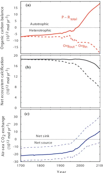
4. Organic carbon balance in the global ocean

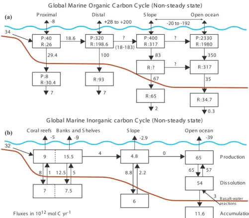
The major driving force of the organic carbon cycle in the global ocean (Fig. 2a) is the production of organic matter by marine primary producers. Some of the estimates of global marine and terrestrial net primary production show that the oceans account for 10

approximately 45% of the organic matter produced globally (Sect. 3). In most oceanic regions, primary production is limited by light intensity and the availability of nutrients, mainly nitrogen and phosphorus, but in some areas by trace elements such as iron. The flux of carbon between the major reservoirs of the global marine organic carbon cycle is controlled by the magnitude of primary production, the extent of respiration and 15

decay, and physical transport processes (Fig. 2a). 4.1. Net ecosystem production

The “ecological” concept of net ecosystem production (NEP) is the net change in or-ganic carbon in an ecosystem over a period of time, usually one year. NEP in a system at steady state is the difference between the rates of gross primary production (P) and 20

total respiration (R_total); the latter is total ecosystem production of inorganic carbon by autotrophic and heterotrophic respiration, including aerobic respiration, decay, decom-position or remineralization (e.g. Smith and Mackenzie, 1987; Smith and Hollibaugh, 1993; Woodwell, 1995; Mackenzie et al., 1998):

NEP=P−R_total. (8)

(18)

BGD

1, 27–85, 2004

Full Screen / Esc

Print Version

Because NEP is the difference between two very large fluxes of gross primary produc-tion and total respiraproduc-tion, both of which are poorly known, it is very difficult to evaluate it from direct measurements.

A system at steady state is “net heterotrophic” when the amount of organic carbon respired, decayed, and decomposed is greater than the amount produced by gross 5

photosynthesis: NEP<0. A system is “net autotrophic” when the amount of carbon fixed by gross photosynthesis exceeds that remineralized by respiration: NEP>0. The net result is either a drawdown (net autotrophy) or evolution (net heterotrophy) of CO₂ owing simply to organic metabolism in the ecosystem.

As mentioned above, a survey of estimates of rates of primary production and total 10

respiration shows that P and R_total do not differ significantly one from another and the difference P−R_totalis practically indistinguishable from zero by evaluation of P and R_totalindividually. The oceanic coastal zone, of an areal extent of 7 to 10% of the ocean surface and a mean depth of about 130 m (e.g. Ver et al., 1999; Rabouille et al., 2001; Lerman et al., 2004) receives a large input of organic matter from land that is added 15

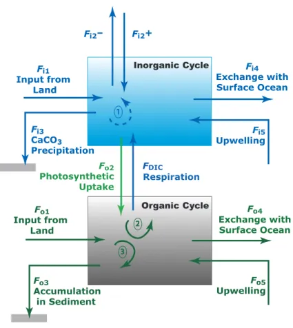
to the organic matter produced in situ. For this budgetary reason, NEP of the oceanic coastal zone exerts a relatively greater control of the carbon cycle in this domain. From considerations of the material carbon balance (Fig. 3), NEP in the coastal ocean is derived from all sources and sinks of particulate and dissolved organic carbon, i.e. input from rivers, upwelling from intermediate oceanic waters, export to the open ocean, and 20

burial in sediments. The material balance for the organic carbon reservoir in the coastal zone is (e.g. Smith and Hollibaugh, 1993; Mackenzie et al., 1998):

d C_org

d t =(Fo1+Fo2+Fo5)−(Fo4+Fo3+FDIC) (mol yr

−1_), ₍₉₎

where C_org is the mass of organic carbon in the reservoir and t is time. Gross photo-synthesis (F_o2) and respiration and decay (F_DIC) are the linkages between the organic 25

(19)

BGD

1, 27–85, 2004

Full Screen / Esc

Print Version

be defined as:

NEP=F_o2−F_DIC_{= (F}_o3_+F_o4) − (F_o1+F_o5) . (10)

For a system in a transient state (d C_org/d t6=0), NEP∗ can be defined as:

NE P∗_{= F}_o2− F_DIC_{= ∆C}_org

t+ (Fo3+ Fo4) − (Fo1+ Fo5) (11) where the difference between NEP∗ and NEP is ∆C_org, the accumulation or loss of 5

organic carbon in the reservoir per unit time. While NEP∗ and NEP can be negative, zero or positive, NEP∗ can theoretically be positive when NEP is negative. NEP∗ is essentially equivalent to the term for non-steady state net biome production (NBP) as used by terrestrial ecologists for changes in the size of the terrestrial carbon pool and thus non-zero NBP. It should be emphasized that we employ NEP∗ in the following 10

model calculations for the coastal zone because there is no a priori reason to assume that the coastal zone organic carbon cycle is in steady state when viewed on the time scale of decades to centuries. Indeed short time scale, direct observations of P and R may be misleading in terms of interpretation of the trophic status of a system that is evolving with time. In addition, because we know that dissolved organic carbon 15

(DOC) in the ocean has a mean age of about 1000 years (Bauer et al., 1992) and is being stored in certain regions of the ocean (Church et al., 2002), it is unlikely that the organic carbon cycle in the ocean is in a steady state, although whether the situation is a long-term or transient phenomenon is unknown.

4.2. Estimates of the organic carbon balance 20

Several investigators have made reasonable estimates of the net global exchange of CO₂ between the ocean and the atmosphere due to organic metabolism for the pre-anthropogenic global ocean, calculated from the small difference between the large biogeochemical fluxes of gross primary production and total ecosystem autotrophic and heterotrophic respiration. Because these earlier estimates shared common sources of 25

(20)

BGD

1, 27–85, 2004

Full Screen / Esc

Print Version

data for the biogeochemical flux components used in the calculations, it is not surpris-ing that the earlier estimates agreed well with each other in both the magnitude and di-rection of the net flux of carbon. Estimation of net ecosystem production in a transient-state system (NEP∗) requires knowledge of the rate of organic carbon change, ∆C_org in Eq. (11), that is not usually available. Therefore the estimates of net ecosystem 5

production discussed below refer to NEP, as given in Eq. (10). Garrels and Mackenzie (1972) estimated that the global ocean was a net source of CO₂to the atmosphere in pristine time at the rate of −27×1012 moles C yr−1 due to organic metabolism. Smith and Mackenzie (1987) concluded that because of aerobic and anaerobic respiration and remineralization of organic carbon exceeding in situ gross photosynthesis, the 10

pre-industrial global ocean was a net heterotrophic system, hence a source of CO₂ with a calculated flux of −21×1012mol C yr1. Organic carbon transported from land via rivers and remineralization of a portion of that carbon in the ocean fueled in part the heterotrophy of the global ocean. Calculations by Wollast and Mackenzie (1989) and Smith and Hollibaugh (1993) based on biogeochemical processes involving organic 15

carbon showed a net flux of about −22×1012 mol C yr−1 from the heterotrophic ocean to the atmosphere. Williams and Bower (1999) calculated from Duarte and Agusti’s data (1998) on bacterial respiration and net primary production that the oceanic sur-face layer should be net heterotrophic by as much as −500×1012 mol C yr−1, a result disputed by the four authors themselves but defended by Duarte et al. (1999). More 20

recently, Ducklow and McAllister (2004) concluded that the open ocean over the entire water column is heterotrophic by −200×1012mol C yr−1.

There have only been a few attempts to estimate either the long-term or present-day NEP of the coastal ocean separately from that of the open ocean. One of the primary reasons is that the transfer fluxes between the coastal margin and the open ocean are 25

poorly constrained (Gattuso et al., 1998). Additionally, it is difficult to model the coastal oceanic region separately from the open ocean because of its large spatial and tempo-ral variability (Mantoura et al., 1991). Furthermore, there may be differences between the proximal and distal parts of the coastal zone: the proximal part (surface area:

(21)

BGD

1, 27–85, 2004

Full Screen / Esc

Print Version

1.8×1012 m2) represents the bays, lagoons, estuaries, deltas, and marine wetlands and the distal (surface area: 27×1012 m2) includes the continental shelves (Fig. 2a). Despite these difficulties, two of the most notable and frequently cited estimates of coastal ocean NEP (Smith and Hollibaugh, 1993; Wollast and Mackenzie, 1989) in-dependently concluded that the coastal ocean was net heterotrophic in pre-industrial 5

times. Wollast and Mackenzie’s (1989) estimated heterotrophy in the global ocean in-cluded a coastal ocean that was heterotrophic at the rate of −3.3×1012 moles C yr−1. Smith and Hollibaugh (1993) and Smith (1995) also calculated the coastal zone to be net heterotrophic at the rate of −7×1012 moles C yr−1. Pre-industrial coastal zone heterotrophy was estimated at −8×1012moles C yr−1by Mackenzie et al. (1998) from 10

the long-term rates of primary production, respiration, net metabolism, river loading of organic carbon, organic carbon burial, and chemical reactivity of terrestrial organic matter. Gattuso et al. (1998) estimated that the present-day continental shelves have a positive metabolic balance, such that NEP is equivalent to+68×1012 mol yr−1. They further estimated that estuarine net ecosystem production amounted to −8×1012mol C 15

yr−1. In a global model developed for the coastal ocean of the interactive biogeochem-ical cycles of C, N, and O, Rabouille et al. (2001) estimated that the pre-anthropogenic nearshore (proximal) coastal zone of the ocean was net heterotrophic by −8.4×1012 mol C yr−1 and that the pre-anthropogenic distal continental shelf was net autotrophic by+28.4×1012mol C yr−1. Finally, Ducklow and McCallister (2004) estimated recently 20

that the present-day global coastal ocean is net autotrophic based on estimates of inputs and outputs of organic carbon by+175×1012mol C yr−1.

In conclusion it appears that the present-day proximal coastal zone is net het-erotrophic by a small amount, the distal continental shelf net autotrophic, the degree to which is controversial, and the open ocean over its whole depth significantly het-25

erotrophic. The past NEP of the coastal zone is still a matter of conjecture but in Sect. 6.3, we adopt for modeling purposes a pre-industrial coastal ocean that is slightly heterotrophic throughout its extent and explain the implications of doing so.

(22)

BGD

1, 27–85, 2004

Full Screen / Esc

Print Version

The shallow-water marine inorganic carbon cycle constitutes a significant part of the global marine inorganic carbon cycle (Fig. 2b). Approximately 25% of calcium car-bonate produced globally is produced within the global coastal ocean and almost 50% of the calcium carbonate that accumulates in global marine sediments accumulates 5

within this region (Fig. 2b) because of some dissolution of deep-sea carbonates (Mil-liman, 1993; Wollast, 1994, 1998). About half of this accumulation is in regions of coral reefs. According to Milliman (1993), accumulation of calcium carbonate miner-als in the coastal ocean is currently unusually high owing to the significant rise in sea level since the Last Glacial Maximum 18 000 yr ago and the subsequent expansion of 10

shallow-water depositional environments. Thus, the global marine inorganic carbon cy-cle currently may be in a non-steady state, where more calcium carbonate is deposited in marine sediments than is added to the ocean via river input and basalt-seawater interactions (Fig. 2b). In the pre-industrial world, release of CO₂ from the oceans to the atmosphere due to CaCO₃deposition is necessary to balance that CO₂consumed 15

by the weathering of carbonates. The non-steady state condition may have been re-sponsible for some of the rise in atmospheric CO₂since the last glacial maximum to pre-industrial time as CaCO₃ accumulated in shallow-water environments during the sea level rise and CO₂ was vented to the atmosphere. This conclusion is still a mat-ter of debate (e.g. Berger, 1982; Keir and Berger, 1985; Milliman, 1993; Opdyke and 20

Walker, 1992; Walker and Opdyke, 1995; Broecker and Henderson, 1998).

The marine inorganic carbon cycle is strongly coupled to the marine organic car-bon cycle through primary production and remineralization of organic matter (Fig. 3). Consequently, direct alterations to either one of these cycles owing to natural or an-thropogenic factors are likely to affect the other.

25

From experimental evidence and geochemical modeling, it has been suggested that the saturation state of surface ocean waters with respect to carbonate minerals will decline during the twenty-first century owing to increased invasion of atmospheric CO₂

(23)

BGD

1, 27–85, 2004

Full Screen / Esc

Print Version

(e.g. Andersson et al., 2003; Kleypas et al., 1999; Mackenzie et al., 2000). The de-gree of supersaturation of surface ocean water with respect to calcite has decreased 15 to 19% as a result of atmospheric CO₂ rise from 280 ppmv in pre-industrial time to 370 ppmv in the present (Sect. 6.1). Although data are sparse globally, monthly observations from the Hawaii Ocean Time series station (HOT, located in the North 5

Pacific subtropical gyre) between 1988 and 2000 indicate a consistent annual trend of increasing surface water total DIC and decreasing carbonate saturation state (Hawaii Ocean Time series, 2003; Winn et al., 1998; Andersson, 2003). This situation has also been observed in other regions of the ocean (e.g. Chung et el., 2004).

Decreasing surface water carbonate saturation state could negatively affect the abil-10

ity of calcareous organisms, such as corals, coralline algae, coccolithophorids, and other taxa, to produce skeletons, shells, and tests out of calcium carbonate and it may result in calcareous organisms and structures being weaker and more vulnerable to environmental stress and erosion. Consequently, the role and function of calcareous ecosystems and communities may be altered as a result of future changing environ-15

mental conditions (Gattuso et al., 1999; Kleypas et al., 1999, 2001; Riebesell et al., 2000; Langdon et al, 2000; Mackenzie et al., 2000; Leclercq et al., 2000, 2002; Ander-sson et al., 2003).

At present, calcium carbonate is almost exclusively produced by calcareous organ-isms and only minor quantities are produced abiotically as cements within sediments 20

or precipitated as whitings from the water column (e.g. Morse and Mackenzie, 1990; Milliman, 1993; Wollast, 1994; Iglesias-Rodriguez et al., 2002). Decreased carbon-ate saturation stcarbon-ate and consequent decreased production of calcium carboncarbon-ate may significantly alter the global marine inorganic carbon cycle and also affect the marine organic carbon cycle. Decreased calcification also implies a decreased flux of CO₂ to 25

the atmosphere owing to this process (Ware et al., 1992; Frankignoulle et al., 1994) and could act as a negative feedback to increasing atmospheric CO₂ (Zondervan et al., 2001). However, the magnitude of this feedback is insignificant relative to the total invasion of anthropogenic CO₂into the surface ocean, as discussed in more detail in

(24)

BGD

1, 27–85, 2004

Full Screen / Esc

Print Version

Sect. 6.

Ultimately, decreasing surface and pore water carbonate saturation state may cause increased dissolution of carbonate minerals in the water column and within the pore water-sediment system. Such dissolution, in particular of metastable carbonate min-erals such as high-magnesian calcite, that is unstable relative to calcite, could act as 5

a buffer to neutralize anthropogenic CO₂and prevent at least some of the negative ef-fects on calcareous organisms and ecosystems (Garrels and Mackenzie, 1981; Barnes and Cuff, 2000; Halley and Yates, 2000). Indeed it has been suggested that the rate of carbonate dissolution might equal the rate of calcification once atmospheric CO₂ con-centration reached double pre-industrial levels and buffer the surface water from rising 10

atmospheric CO₂ levels (Halley and Yates, 2000). However, recent model results in-dicate that such dissolution will not produce sufficient alkalinity and anthropogenically-induced changes in coastal ocean saturation state will not be restored by the dissolu-tion of metastable carbonate minerals (Andersson et al., 2003). Thus, most investiga-tors believe that calcification by calcareous marine organisms and the development of 15

carbonate reefs could be negatively affected as a consequence of rising anthropogenic CO₂and lowering of the saturation state of seawater with respect to carbonate miner-als (Gattuso et al., 1999; Kleypas et al., 1999; Mackenzie et al., 2000; Langdon et al., 2000; Leclercq et al., 2002).

During early diagenetic modifications on the seafloor, dissolution of carbonate min-20

erals follows a sequence based on mineral thermodynamic stability, progressively lead-ing to removal of the more soluble phases until the stable phases remain (Schmalz and Chave, 1963; Neumann, 1965; Wollast et al., 1980). Thus increased dissolution of car-bonate minerals owing to anthropogenically-induced changes in carcar-bonate saturation state of the coastal ocean can potentially affect the average CaCO₃composition (its Mg 25

content) and rates of precipitation of carbonate cements in contemporary shallow-water marine sediments (Andersson et al., 2003). However, it should be pointed out that the extent of carbonate dissolution is mainly controlled by microbial remineralization of or-ganic matter producing CO₂ rather than the carbonate reaction kinetics (Morse and

(25)

BGD

1, 27–85, 2004

Full Screen / Esc

Print Version

Mackenzie, 1990). Increased transport and deposition of organic matter to the sedi-ments of the coastal zone (Mackenzie et al., 1993; Meybeck, 1982) and/or subsequent changes in the NEP∗could therefore have an important effect on the carbonate content and composition of marine sediments.

6. Rising atmospheric CO₂and air-sea exchange of CO₂ 5

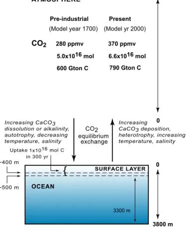
Net increase in atmospheric CO₂due to fossil fuel burning and land-use changes was from 280 ppmv CO₂to 370 ppmv by the end of the 20th century. Total CO₂ addition to the atmosphere by the year 2000 has been estimated at 461±19 Gton C (3.84×1016 mol C), of which 134±6 Gton (1.12×1016 mol) were taken up by land ecosystems, leaving 327±13 Gton (2.72×1016 mol) to be distributed between the atmosphere and 10

the ocean. Of these, an estimated 122±2 Gton C (1.02×1016 mol) were transferred to the ocean, leaving 205±13 Gton C (1.71×1016 mol) in the atmosphere (Ver et al., 1999; Mackenzie et al., 2001; see also Sarmiento et al., 1992; Hudson et al., 1994; Bruno and Joos, 1997).

We address three questions based on modeling calculations of the carbon cycle 15

related to the increase in atmospheric CO₂during industrial time of the past 300 years: 1. What were the changes in the ocean-water carbonate system due to the increase

in atmospheric CO₂?

2. What was the thickness of the surface ocean layer that absorbed the increased CO₂?

20

3. What has been the history of the CO₂exchange flux between the shallow-ocean environment and the atmosphere?

The inorganic carbon balance in the atmosphere and ocean, with their thicknesses drawn to scale in Fig. 4, shows an increase in atmospheric CO₂ during the industrial period of 300 years and uptake of CO₂by the surface ocean layer, as will be discussed 25

(26)

BGD

1, 27–85, 2004

Full Screen / Esc

Print Version

in more detail later in this section. In Fig. 4 are also shown the main inorganic and organic processes that can be responsible for the direction of CO₂ flow between the ocean and atmosphere: the previously discussed role of heterotrophic respiration and CaCO₃ precipitation in producing excess CO₂in water and its subsequent transfer to the atmosphere; conversely, transfer of CO₂ from the atmosphere to surface water by 5

an increasing autotrophic production or its increasing alkalinity and/or CaCO₃ dissolu-tion; and the effects on the direction of transfer due to the dependence of CO₂solubility on temperature and salinity.

6.1. Air and surface ocean system

The simplest approximation to the distribution of CO₂ between the atmosphere and 10

surface ocean water is a solubility equilibrium at a certain temperature:

K₀0=[CO2] P_CO

2

, (12)

where [CO₂] is concentration of dissolved CO₂species (mol/kg), P_CO

2 is atmospheric partial pressure of CO₂ (bar) at equilibrium with solution, and K₀0 is the temperature-dependent solubility coefficient (mol kg−1 bar−1). The concept of a chemical equilib-15

rium is only an approximation to the atmosphere in contact with surface ocean water because of several factors: ocean surface temperature varies with latitude and CO₂ sol-ubility increases at lower temperatures and lower salinities; oceanic sections of deeper water upwelling are often sources of CO₂emissions to the atmosphere, whereas the downwelling areas, such as the North Atlantic, are sinks of atmospheric CO₂ trans-20

porting it into the deeper waters; and global balance of directions of CO₂flows across the ocean-air interface shows large parts of the Northern and Southern hemispheres as CO₂sinks and regions in the lower, warmer latitudes as sources (Takahashi, 1989; Chester, 2000). In general, as has also been discussed in the preceding sections, min-eralization or oxidation of organic matter brought from land to the surface ocean is a 25

(27)

BGD

1, 27–85, 2004

Full Screen / Esc

Print Version

processes releases CO₂ into ocean water; and primary production in surface waters, consuming dissolved CO₂, may create at least temporarily a disequilibrium between the atmosphere and ocean water.

For a rise in atmospheric P_CO

2 from 280 to 370 ppmv, dissolved [CO2] concentration also increases and, as shown in Table 2, the increase at 5◦C is greater than at 25◦C 5

because of the higher solubility of CO₂ at lower temperatures. The higher concentra-tion of dissolved CO₂ would result in an increase in total dissolved inorganic carbon (DIC), changes in the [H+]-ion concentration, and changes in the concentrations of the individual dissolved carbonate species [HCO−₃], [CO2−₃ ], and [CO₂]. Assuming that dur-ing the period of ≤300 years, the total alkalinity (A_T) of surface ocean water remained 10

constant (that is, no significant amounts of carbonate precipitation or dissolution or ad-dition of alkalinity from land are considered), the new values of ocean water pH and DIC at the higher atmospheric P_CO

2 are given in Table 2. The calculation is based on the relationships discussed below.

The values of total alkalinity, A_T, and concentration of dissolved inorganic carbon 15

(DIC) are defined by the following relationships:

A_T=A_C+A_B+A_w (mol/kg) (13) A_T=[CO2]K 0 1 [H+] 1+ 2K₂0 [H+] ! + BT 1+[H+]/K_B0+ K_w0 [H+]−[H +_], ₍₁₄₎

where A_C is carbonate alkalinity, also represented by the first term on the right-hand side of Eq. (14); A_B is borate alkalinity, as in the second term in Eq. (14), where B_T 20

is total boron concentration in ocean water; A_w is water or hydrogen alkalinity, repre-sented by the last two terms in Eq. (14); and the definitions and values of the apparent dissociation constants, K0, are given in Table 3.

[DIC]=[CO₂]+[HCO−₃]+[CO2−₃ ]=P_CO 2K 0 0 1+ K₁0 [H+]+ K₁0K₂0 [H+]2 ! (mol/kg). (15)

(28)

BGD

1, 27–85, 2004

Full Screen / Esc

Print Version

In this model of CO₂ uptake from the atmosphere at an equilibrium with a surface ocean layer, the initial atmospheric CO₂ of 280 ppmv and an assumed pH=8.20 at 25◦C give the total alkalinity A_T=2.544×10−3mol/kg that we consider constant. At other combinations of temperature and atmospheric P_CO

2, the hydrogen-ion concentration, [H+], is obtained by solution of Eq. (14) and new DIC concentration computed from 5

Eq. (15). At these conditions, carbonate alkalinity (A_C) accounts for a major part, 95 to 97%, of total alkalinity (A_T). To estimate the degree of saturation of ocean water with respect to calcite (Ω), the carbonate-ion concentration that depends on P_CO

2 and [H +_], [CO2−₃ ]=[CO2] K 0 1K 0 2 [H+]2 (mol/kg) (16)

and constant calcium-ion concentration of [Ca2+]=1.028×10−2mol/kg are used in 10

Ω=[Ca

2+

][CO2−₃ ]

K_cal0 (17)

the results of which are also given in Table 2 for the pre-industrial and present-day conditions.

6.2. Industrial CO₂surface ocean layer

An increase in atmospheric CO₂from the pre-industrial value of 280 ppmv to 370 ppmv 15

in the present results in an increase of DIC by 2.6 to 1.7%, lowering of the pH by about 0.1 unit, and a decrease in the [CO2−₃ ]-ion concentration (Table 2). The latter is responsible for the lowering of the degree of supersaturation of surface ocean water with respect to calcite, both at 25 and 5◦C. It should be noted that the increase in DIC represents the total mass of carbon transferred from the atmosphere as CO₂to ocean 20

water, where the added CO₂ causes an increase in concentration of the H+-ion and changes in the concentrations of dissolved species [CO₂], [HCO−₃], and [CO2−₃ ]. Thus

(29)

BGD

1, 27–85, 2004

Full Screen / Esc

Print Version

only a fraction of atmospheric CO₂gas becomes dissolved [CO₂] at equilibrium with the atmosphere, whereas most of the increase goes into the bicarbonate ion, increasing DIC. The increase in DIC at 25 and 5◦ is, from Table 2:

∆[DIC]=[DIC]P_CO2=370−[DIC]P_CO2=280

=2.162×10−3_−2.092×10−3_=6.9×10−5_{mol C/kg at 25}◦_C

5

=2.352×10−3_−2.300×10−3_=5.2×10−5_{mol C/kg at 5}◦_C.

The thickness of the surface ocean layer that takes up CO₂ from the atmosphere de-pends on the mass of carbon transferred from the atmosphere, as cited at the beginning of Sect. 6, ∆n_a≈1×1016mol C, and the increase in DIC concentration within a water layer of mass M_w:

10

∆na=∆[DIC]×Mw (mol C). (18)

Thus the thickness of the surface ocean layer, h, where dissolved CO₂ is equilibrated with the atmosphere, is from Eq. (18):

h₂₅◦_C=(1×1016mol C)/(6.9×10−5×1027×3.61×1014)=390 m

h₅◦_C=(1×1016 mol C)/(5.2×10−5×1027×3.61×1014)=518 m, 15

where the mean density of ocean water is taken as 1027 kg/m3and ocean surface area is 3.61×1014m2.

The above results for a 390 to 520-m-thick surface ocean layer are constrained by an external estimate of the carbon mass transferred to the ocean in industrial time, about 1×1016mol C, and by our conceptual model that assumes an equilibrium be-20

tween atmospheric and dissolved CO₂ in a water layer where total alkalinity remained constant (compare this model of the surface layer with Fig. 3 that shows carbon flows in the coastal zone). Lower total alkalinity would increase the surface layer thickness,

(30)

BGD

1, 27–85, 2004

Full Screen / Esc

Print Version

at the same mass of industrial-age CO₂stored in the ocean: at the total alkalinity value of 2.300×10−3instead of 2.544×10−3used in the above computation and Table 3, the surface layer thickness would be about 430 m at 25◦C or 580 m at 5◦C.

In a 400 to 500-m-thick water layer, the mass of DIC in pre-industrial time was be-tween 31 and 43×1016mol C, and it increased by 1×1016mol at the expense of atmo-5

spheric CO₂ in 300 years. In the same period, the mass of carbon supplied by rivers to the ocean would have been between 0.4×1016 and 1×1016 mol C: this estimate is based on the HCO−₃ ion concentration in rivers from 23 mg/kg (HCO−₃ from dissolution of carbonate rocks only; Drever, 1988; Mackenzie, 1992) to a total concentration of 52 mg/kg (Livingston, 1963; Mackenzie and Garrels, 1971; Drever, 1998; Berner and 10

Berner, 1996), and a global water discharge to the ocean of 3.74×1016 kg/yr (Baum-gartner and Reichel, 1975; Meybeck, 1979, 1984; Gleick, 1993). Net removal rate of CaCO₃ from ocean water is its storage in shallow and deep-water sediments at the rate of 32.1×1012 mol/yr (Fig. 2b) and corresponds to removal in 300 years of nearly 1×1016 mol C from ocean water. This seeming balance of inorganic carbon input and 15

removal is not supported by the estimates of CO₂ evasion from the ocean (Fig. 2b) that, although not addressing the industrial rise of atmospheric CO₂, indicate the inor-ganic carbon input as being less than needed to account for the CaCO₃ precipitation. Similarly, the delivery of organic carbon by rivers at the rate of 26 to 34×1012 mol/yr (Ver et al., 1999; Fig. 2a) produces in 300 years an input of 0.8 to 1×1016 mol C. Its 20

storage as organic matter in sediments at the rate of 8 to 16×1012 mol/yr (Ver et al., 1999; Fig. 2a) corresponds to removal of 0.2 to 0.5×1016 mol C from ocean water in 300 years.

The preceding estimates suggest that addition of inorganic and organic carbon from land to the ocean in the past 300 years was 1.8 to 2.0×1016 mol C, which is close 25

to, but possibly somewhat greater than, the removal of carbonate and organic carbon by net storage in sediments, 1.2 to 1.5×1016 mol C. Despite the uncertainties in these estimates of the in and out carbon fluxes, the evasion flux of CO₂, and the nature of our air-water exchange model for the industrial age, we reiterate that the calculated mass