Neighbor-of-Neighbor Routing In Small-World Networks With Power-Law Degree

(1)

HAL Id: dumas-00854954

https://dumas.ccsd.cnrs.fr/dumas-00854954

Submitted on 28 Aug 2013

HAL is a multi-disciplinary open access

archive for the deposit and dissemination of sci-entific research documents, whether they are pub-lished or not. The documents may come from teaching and research institutions in France or abroad, or from public or private research centers.

L’archive ouverte pluridisciplinaire HAL, est destinée au dépôt et à la diffusion de documents scientifiques de niveau recherche, publiés ou non, émanant des établissements d’enseignement et de recherche français ou étrangers, des laboratoires publics ou privés.

Neighbor-of-Neighbor Routing In Small-World Networks

With Power-Law Degree

Olivier Ruas

To cite this version:

Olivier Ruas. Neighbor-of-Neighbor Routing In Small-World Networks With Power-Law Degree. Dis-tributed, Parallel, and Cluster Computing [cs.DC]. 2013. �dumas-00854954�

(2)

Research Master’s Degree Internship Report

Neighbor-of-Neighbor Routing In Small-World Networks With

Power-Law Degree

Author : Olivier Ruas Supervisors : George Giakkoupis Anne-Marie Kermarrec Team : ASAP

(3)

Abstract

During this internship we have studied decentralized routing in small-world networks. Our model is an variant of Kleinberg’s model: we use a 1-dimensional grid in which the number of long-range contacts is not a constant but instead follows a power law probability distribution, the edges are considered bidirectional and drawn independently: they follow a harmonic distribution as in Fraigniaud and Giakkoupis work ([13]). We increase the number of neighbors to an expected O(ln n) number of neighbors instead of a constant expectation as in the previous work. We also increase knowledge to every node: they know the neighbors of their neighbors. This model was motivated by Kleinberg in [16] and by the work of Manku, Naor and Wieder ([23]) who have shown that this improves the efficiency of routing to an optimal expected value in their model. We proved that the expected number of steps for routing a message in this model using a greedy algorithm, with respect to the knowledge the nodes have, is O(1) which is optimal.

Keywords. Small-world networks, Random graphs, Probabilities, Routing, Distributed algo-rithm.

(4)

1 Introduction

The aim of the internship was to improve the efficiency of a greedy routing algorithm in an existing network. To achieve this we have employed two ideas already used on this network which have lead to a great improvement of the routing efficiency. The particularity of this work is that we used this ideas together instead of separately.

1.1 State of the art

The study of complex networks is interesting since they are more and more used in a wide range of fields. For instance social networks are an example of complex network difficult to study due to their informal definition and can be applied to a lot of different models of networks. We focus on small-world networks which are networks in which there are short paths between almost all pairs of nodes. We can model such networks by random graphs, which are well studied in mathematics, using discrete probabilities and combinatorics. We take a node space and we randomly create links between the nodes. The difficult part in proceeding in this way is to obtain graphs with the same properties that the networks we want to study have. In order to achieve this we classify the random graphs by models depending on how they are generated and study the whole model at once.

For each model we want to know how efficient routing a message from a node to another is. This is an interesting problem studied a lot in every model of networks because most of the pro-tocols upon networks are done thanks to message passing, then the efficiency of routing have a huge impact on the efficiency of these protocols. Efficiency is typically measured as the number of hops, or nodes visited by the decentralized algorithm during its execution to find the path from the source to the target. We use this measure of efficiency in this work. The results depend on the model and the algorithm but we focus on greedy decentralized algorithms because they are really simple and have good efficiency. The efficiency of the greedy algorithm is known for a large set of models but these results use different algorithms and protocols which make us think that we could have better complexity with only few changes as combining several ideas together.

1.1.1 The small-world phenomenon

Most of us have already experienced the fact that, while meeting someone far from home, we discover that we share an mutual acquaintance. There is a well-known concept of ”six-degree” of separation between two people which reflects the fact that two people, even far away, can actually be connected through short chains of mutual acquaintances.

The latter common expression comes from an experiment made by Stanley Milgram in the 60’s ([27]). To point out the existence of short paths between people, random people in Omaha (Nebraska) were selected to send a message to the same target in Boston (Massachusetts). They were given few pieces of information about the target such as his name, location and occupation. The participants only have the right to forward the message to someone they know. If the holder of a message does not know the target, he forwards it to the person he knows who is the most likely to know the target. The receiver has to do the same until the message reaches someone knowing the target who, finally, forwards to the target. By only forwarding the message to acquaintances of them, chains of acquaintances between the sources and the target are highlighted (everyone receiving the message had to write his name on the message). The results of the experiment have shown that the length of the chains were from two to ten with a median of five intermediate persons. It was the first time such phenomenon was highlighted and at this time the results were quite surprising.

(6)

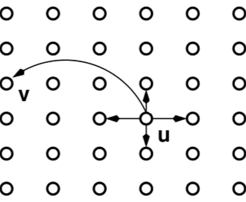
Figure 1: Kleinberg’s network in dimention 2, n = 6, showing the 2 close contacts and the long-range contact of u.

all pairs, since only 44 out of the 160 letters reached the target and there was an unique target which seemed to know a lot of people (he was not randomly selected). Still we can wonder what we can learn from this experiment; by seeing every person as a node and the acquaintanceship as an edge, we obtain an interesting property about the resulting network : not only there exists short paths between every pair of nodes but nodes can construct them only by knowing local information which means that a greedy algorithm should be efficient to find short paths in the network we get. Such a network (i.e. in which there are short paths between almost every pair of nodes) is called a ”small-world” network.

The study of these networks is useful since they can model several real networks: the collab-oration graph of film actors, the power-grid of the western United States or the neural network of the worm Caenorhabditis elegans exhibit the small-world property for example ([2], [8], [28], [31], [20], [22]).

1.1.2 Kleinberg’s model

Modeling a small-world network is not that easy; just taking a graph with random neighbors for every node is not efficient because such a network does not grasp the property of small-world network which is that most of the friends of a person are friends together. One of the first model was done by Watts and Strogatz ([31]): they took n nodes spaced uniformly on a ring and, using the natural L1 distance associated, every node was linked to its k closest neighbors (where k

is a small constant) and to a fixed number of random nodes which were selected uniformly at random across the network. This network was grasping the property that the common friends of two nodes are likely to be themselves friends together but without being too clustered so it has a low diameter. Nevertheless, although the short paths exist, Kleinberg ([16], [17]) has shown that in such a network there is no decentralized algorithm capable of constructing paths of small expected length.

So Kleinberg in [16] defined a grid-based model holding the small-world property: n2 nodes are displayed on the two dimensional n × n grid graph, and every node has an edge with the 4 closer nodes (called local contacts) and one other randomly picked node (the long-range con-tact). See Figure 1 for an example (made from a picture in [16]). The main difference with the previous model is that there is a directed edge from u to v with a probability proportional to d(u, v)−r(the previous model is a particular case of this one, with r = 0 and k = 1) where d(u, v) is the L1distance between u and v over the network and r (called the clustering exponent) a real.

(7)

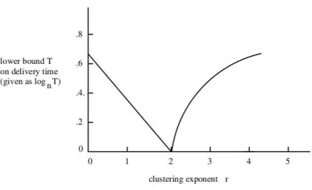
Figure 2: Influence of the clustering exponent on the efficiency.

As the nodes only know the location of their acquaintances and the target, without knowing anything else about the network, the greedy algorithm works as follows : we simply forward the message to your neighbor which is the closest to the target and this node will have to do the same until the message reaches the target. It has been shown (in [16]) that this greedy routing algorithm, which is decentralized, reaches the target in:

• Ω(n2−r3 ) hops in average for 0 ≤ r < 2

• Ω(nr−2r−1_{) for 2 < r}

• O(log2n) for r = 2

We can see r as an expression of the correlation between the local structure and long-range connections. The Figure 2 (extracted from [16]) shows that 2 is a critical value, for which the long-range contacts are uniformly distributed over distance scales (the probability for the long-range contact to be at a distance between 2i and 2i−1_{is about the same for i ∈ [0.. log n]).} Then when r is close to 2, we have a good chance to halve the distance between the message and the target at each forwarding, regardless of the distance between the source and the desti-nation. If the distribution is too homogenous (i.e. r is lower than 2, as in the first model), nodes can not find short paths although they exist, and if r is above 2, the network is too clustered to have short paths.

1.1.3 Extensions of the model

The above results extend to d-dimensional grid networks ([16]), and the results are similar: the decentralized greedy algorithm can find paths of length polynomial in log n if and only if r = d. This seems normal considering the previous consideration, below d the network is too homogenous, above it is too clustered. For r = d we obtain O(log2(n)) hops in average. For all these models, the variant with a constant number of long-range contacts for each node has been studied and in the models obtained the greedy algorithm has the same asymptotic efficiency.

An other idea was to have a variable number of long-range contacts for every node. It is relevant since in real social networks nodes are very different and do not have the same degree. Fraignaud and Giakkoupis ([11]) have studied such a network : in the d-dimensional grid network, which can be represented by [0..n−1]d, every node has its 2d closest nodes as close

(8)

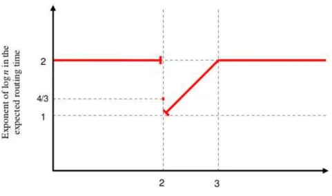
Figure 3: Results of greedy algorithm in undirected graph with variable numbers of neighbors contacts and the number of long-range contacts is randomly chosen. The probability of having k long-range contacts is proportional to _k1α and the expected value is 2, with 0 ≤ α. Then

the directed edges are chosen with the same method as before. This model and the power-law distribution are motivated by the fact that the degree in some real social networks seem to follow a power-law with an exponent between 2 and 3 ([2], [8], [28]).

With this model the greedy algorithm has an expected delivery time of Ω(log2(n)). By making the edges undirected (for each directed edge (u, v), we add the edge (v, u)), the expected delivery time is improved:

• ˜Θ(ln43 n) , if α = 2

• ˜Θ(lnα−1n), if 2 < α < 3 • ˜Θ(ln2n), else

As we can see in Figure 3 (extracted from [11]), by adjusting the value of α, we can get as close as we want of ln n but we can’t reach it.

Until now, the efficiency of the greedy routing algorithm was coming from the homophily of the network : the tendency of individuals to associate with individual similar to them. It is a property we find in real life (you are more likely to know someone in your city that someone living in an other country) and represented in Kleinberg’s network by the close contacts and the harmonic distribution which favors bonds between nodes no too far from each other. By making the number of edges of a node a variable, we add degree disparity which allows some nodes to act like hubs between distant parts of the network.

1.1.4 Leveraging knowledge about neighborhood

The greedy algorithm is based on the fact that you only know the distance of your neighbors from the target and you forward the message to the one who minimizes this distance. Then we can wonder what happens if we get more information about our neighbors, as their own neighborhood. Dodds, Roby and Watts ([7]) made a study similar to Milgram’s in which they asked each participant to say the reasons why they have decided to forward the message to this particular person. It appears that, despite the fact that the location is the first reason for forwarding, in the two first steps about 25% of the forwarding were due to partial knowledge

(9)

about the neighborhood (the neighbor chosen was known to have traveled near the target’s location or has family from this place). Knowing this makes relevant to allow nodes to have more knowledge about the network.

First we consider that nodes know the neighbors of their neighbors. Manku, Naor and Wieder studied ([23]) this assumption over Kleinberg’s original model. In this work, the greedy algorithm does not forward to the node which minimizes the distance with the target but to the one which has a neighbor who minimizes it. We call this method of looking one step further 1-lookahead.

Since in a network with k out-going links per node the average length of short paths is Ω(log n/ log k) ([24]), it should be possible to achieve routing times that match the network diameter of O(log n/ log log n) with k = O(log n). Manku, Naor and Wieder ([23]) have shown that the 1-lookahead policy has really good results and matches this O(log n/ log log n) bound. Since one step lookahead offers paths with an optimal length (because they asymptotically match the network diameter), additional lookahead can not improve the asymptotic length of the paths.

Both of the previous works are interesting and improve the efficiency of the initial model of Kleinberg and our goal in this work is to combine the two mentioned above ideas and to study the new efficiency.

1.2 Our contribution

During this internship we have considered a model based on Fraigniaud and Giakkoupis work ([13]) in which we increase the knowledge of each node. This model is a 1-dimension grid in which each node has a variable number of long-range contacts chosen independently at random from the 1-harmonic distribution. The probability of having k long-range contacts is proportional to 1/k2 with a O(ln n) expectation. We treat the long-range contacts as bidirectional and assume that every node has at least one long-range contact. We study the complexity of the greedy algorithm which is different from the one studied by Kleinberg in ([16]) and Fraigniaud and Giakkoupis in [13] since we add knowledge to every node: every node knows its neighbors and the neighbors of its neighbors. So we will study the same algorithm used in [23] by Manku, Naor and Wieder: a node will not forward to the node which will minimize the distance with the target but to the one who has a neighbor which minimizes it.

In this model and with such protocol we found that the expected number of steps to reach the target from the source is O(1) which is optimal. The proof is detailed in section 6.

1.3 Related work

C. Martel and V. Nguyen have studied networks similar to the grid graph and computed their diameter ([25], [26], [4]) but the grid-based networks are not the only networks which exhibit the small-world property, indeed Kleinberg ([18]) has studied routing in several networks, including a b-tree based network in which the distance between two nodes is based on the height of their lower common ancestor. As the grid was a simple abstraction of geography, this hierarchy is an acceptable abstraction of occupations, hobbies etc... He also proposed a model which generalizes both of the previous ones (the grid-based model and the hierarchical model) by grouping all the nodes by sets: each node may be in multiple sets and the distance between two nodes is based on the size of the smallest set containing both of them.

In all these models, with good distribution of long-range contacts, greedy rooting, with respect to the distance and the topology of the network, reaches the target in polylogarithmic expected number of steps.

D. Liben-Nowell, J.Novak, R. Kumar, P. Raghavan, and A. Tomkins have studied ([22]) a lot of real networks using geographic routing which appear to be small-world networks. They simulate in on of these networks (the LiveJournal social network) Milgram’s experiment. The

(10)

interest was to get rid of human participation which can lead to an addition of noise in the results, e.g. several people did not forward the letters in Milgram’s experiment, and Milgram could not tell the difference between those who have tried to forward but did not find a person and those who did not wanted to participate. Without that noise they were able to verify that individuals were able find short paths only by using geographic information.

In [20], S. Lattanzi, A. Panconesi, and D. Sivakumar have modeled the social networks of co-authorships in computer science. Two persons are friends if there are co-authors and instead of using the geographic distance they used a ”interest” distance to decide which friend you should forward to. They obtained a social network of roughly 15 million of individuals and simulate on it the Milgram’s experiment to show that they network was indeed a small-world network despite the unusual distance used.

There is also a lot of work done to find lower-bounds for greedy routing algorithms in such networks, as [5] by M. Dietzfelbinger, J. Rowe, I. Wegener, and P. Woefel in which they have shown that, with unidirectional links, the expected number of steps for routing is Ω(ln2n) in the ring-based network. In [6], Dietzfelbinger and Woelfel extended this result for a variable number of contacts: no matter the distribution used to drawn the number of long-range contacts of the nodes, as long as the expected number of long-range contacts is a constant the greedy routing need a Ω(ln2n) expected number of steps (our work is not affected by this since we have a O(ln n) expected number of long-range contacts and the edges are bidirectional).

Manku, Naor and Wieder studied ([23]) the 1-lookahead method over several networks (per-colation graph, skip graph, Chord...) and they have shown that using this method in small-world percolation networks leads to an optimal routing of O(_{log log n}log n ) steps.

Adamic and al. ([1]) have worked on efficient routing algorithm on unstructured P2P net-works which have power-law link distribution like Gnutella and Freenet and in which you do not precisely know the location of the target. They have highlighted that the efficiency of the random walker (basically you just randomly forward the message to one of your neighbor until you find the target or until you have reached a chain of a given size) was relying on the existence of high degree nodes so they introduced several algorithms similar to the random walker which aims intentionally these nodes. They proved that their algorithms were sub-linear in the size of the network.

N. Sarshar, P. O. Boykin, and V. P. Roychowdhury have also tried several strategies for routing in unstructured P2P networks.

Simsek and Jensen ([30]) have studied a network similar to the 1-dimensional grid with the power-law distribution but also with the poisson distribution and used an algorithm using both homophily and degree disparity to increase the efficiency of the routing. They design an algorithm which consists in forwarding the message to the node which minimizes the expected length of the path to the target. In practice, since you can not accurately compute this value they use an estimate of it: if the target is one of your neighbors then you forward to it, else your forward the message to your neighbor which has the highest probability of having one of its links ending at the target. This probability can be computed assuming that you know the precise location of the target and those of your neighbors and the degree of your neighbors. They find out that their algorithm was better than the ones using only homophily (e.g. the algorithm used in Kleingberg’s network) or the ones using only degree disparity (e.g. algorithms designed in [1]) but only thanks to simulation, without any theoretical bounds.

B. Kim, C. Yoon, S. Han, and H. Jeong have defined in [15] a new notion on diameter which depends on the strategy used to forward the message and then studied it for several strategies including the one using only local information. They found that using both this strategy and with a global strategy the diameter increases logarithmically with the network size (the network used was the model of Barab´asi and R. Albert ([3]) which is a network with a power-law link distribution).

(11)

do not act the same if you have knowledge about your neighborhood or not. Giakkoupis and Schabanel ([14]), based on the work done in ([21]), have made an algorithm on Kleinberg network which is more complex than the greedy one but in the other hand it finds paths with optimal expected length O(log n) while visiting O(log2+ǫn) nodes, 0 < ǫ fixed, with high probability. The result is the same for the other dimensions than 2, except 1 for which they have proven that the length is O(log n log log n). To achieve this, they keep track with the message of all the nodes which have forwarded the message, allowing a backtrack when needed in order to find the shortest path. With this possibility, they go through a BFS tree starting at the source and they have shown that one of the leaves is closer to the target than the source with some non-null probability. They forward to this node and start again the process until it reaches the target. With that algorithm, since we are forwarding the message to some nodes which will not be a part of the final path, we are not only interested in the length of the found path but also in the number of nodes ”visited” by the message.

On the other hand, Fraigniaud, Gavoille and Paul ([10]) designed a non-greedy routing which improved the length of the path from O(ln2n) (the best we can achieve for greedy routing) to O(ln1+1/d) in the Kleinberg’s d-dimensional grid assuming that you have O(ln2n) bits of topological awareness per node. They proved that the bound is tight.

2 Model

The small-world random graph we use is a 1-dimensional grid of size n. Each node is charac-terized by an integer i ∈ [0..n − 1], the distance between two nodes i and j is then d(i, j) = i − j mod n. Every node is linked to the two nodes which are at distance 1 from him, they are called the local contacts. We add to this graph, which is until now deterministic, some ran-dom directed edges to some further nodes, called long-rang contacts: a node has k long-range contacts with a probability proportional to _k12, and then the k long-range contacts are chosen

independently at random with replacement following a distribution that links two nodes i and j 6= i with a probability proportional to d(i,j)1 .

More precisely the power-law distribution from which the number of long-range contacts of u is drawn, called Cu, is defined as follows:

Pr(Cu = k) = _kc2

where c is a normalizing constant. The average number of long-range contacts is O(ln n) so it leads to: E(Cu) = n−1P k=1k · c k2 = c · (ln(n − 1) + γ + o(1)) = O(c · ln n)

which implies c = Θ(1) so we finally have Pr(Cu = k) = Θ(_k12).

For the distribution from which the long-range contacts are independently drawn is the same as in Kleinberg’s initial network:

Pr(u → v) = _c′_·d(u,v)1

where c′ is a normalizing constant. The sum of all the probabilities equals to one, so we have :

c′ ₌ P v6=u

1

d(u,v) = Θ(ln n)

(12)

Figure 4: Distant neighborhood of u. Directed links : (u,A) (u,B) and (C,u).

3 Neighbor-to-Neighbor Algorithm in our Model

To improve the efficiency of the routing, we ignore the direction of edges: if there is a directed edge from u to v, v will be able to use it to forward a message to u even if there is no edge from v to u as in the model of Fraigniaud and Giakkoupis ([13]). Due to this, the neighborhood is not only composed by the out-going contact of the nodes, but also by all the node for which you are an out-contact (e.g. if there is a directed link from u to v, u is in the neighborhood of u as we can see in figure 4, there is a link from C to u but C is a part of the neighborhood u). Neighborhood is then a symmetric notion.

Every node know the structure of the underlying network (1-dimensional grid of size n), the exact location of the target, all its neighbors, the neighbors of its neighbors (and the links between them) in the network. This knowledge allows every node to compute the distance to every node it knows to each other ant to the target.

With such knowledge, instead of forwarding to its neighbor which is the closest of the target, we look at all the neighbors of our neighbors, select the one which is the closest and forward to it via one of their common neighbor. A node will forward to one of its direct neighbors only if it is the source, indeed if it is not, thanks to the local contacts we are sure to the existence of one neighbor of one of its neighbors which is closer from the target. Thus the message is going through the network two steps by two, excepted maybe the last forwarding:

It is exactly the same algorithm called Neighbor-of-Neighbor (NoN) greedy routing algorithm studied by Manku, Naor and Wieder in [23]. See Figure 5 to see an example of how the algorithm works.

4 Results

Our main result is the following theorem:

(13)

Algorithm 1 The routing protocol to forward a message to node t if _{Current node 6= t then}

Let N1..Nj be the neighbors of the current node.

if Target = Nk then

Forward to Nk

else

Let Nk1..Nkj′ be the neighbors of Nk ∀k ∈ [1..j].

Select the Nki which is the closest to t.

Forward the message to Nki via Nk.

end if end if

Figure 5: The first two steps of the algorithm : u0 want to send a message to t, uses v0 to

(14)

contacts following a power-law distribution of exposant 2 and the links are independently drawn following an harmonic distribution, the expected number of steps needed for a message to reach its target using the NoN-greedy routing algorithm is O(1) which means it is independent of the size of the network. This result is the optimas we can achieve for a routing algorithm.

4.1 Notations

Due to the fact that the message is going through the network two steps by two, we have to make a distinction between two kinds of nodes : first we have the nodes ui; they are receiving

the message (or the source) and they will execute the main algorithm until it finds the target. Then we have the nodes vi; they will only forward to one of their neighbors which has already

been chosen by the ui which have forwarded the message to vi.

One interesting property is that on the path u0..ui (we do not write the vi but we must not

forget that between any ui and ui+1their exists a common neighbor vi, linked to both), for any k

we have d(uk, t) > d(uk+1, t) but we can not say anything about the distance from any vkto any

other v′

k and to the target. The only information we have about vk is that d(vi, t) > d(ui+1, t)

because if it we had d(vi, t) ≥ d(ui+1, t), ui would not have forwarded the message to ui+1since

at least one node was closer from the target: one of the local contacts of v.

A ball of radius r, centered on t is written Bt(r). It is the set of all the nodes in the networks

which are at a distance lower than r from t, formally: Bt(r) = {v | d(v, t) ≤ r}

4.2 Intuition of the proof

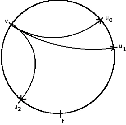
The entire proof works on the fact that the edges are bidirectional: indeed, thanks to that we do not have to consider the edges going from the source but we just have to look at all the other nodes and bound the probability that one of them is linked to both the node which has the message and to a ball of a given size centered on the target. For an example of such a node see figure 6 in which u is the source, t the target and the ball is represented in blue.

The efficiency comes from the fact that there are several nodes with high-degree: they will act like hubs although they should be really far from both the node which has the message and the target. The 1-lookahead policy allows the nodes to know if such a node is in its neighborhood. Then the holder of the message selects among the possible hubs the one which will forward the message to the closest node from the target. Most of the time, especially when the message holder is far from the target, these hubs are the important nodes since they are the most likely to have an edge to the targeted ball.

In other words what really matters is not which nodes the holder of the message is linked to but which nodes are linked to him. The difficulty is coming from the path: if the links were unidirectional (that is not exactly our case since, for an edge (u, v) we can use it as is was (v, u)), the path used to reach a node does not have much influence on what the node will do since its links are independent of the links of the ones of the path (because they are unidirectional), then we have a Markov’s chain. But here we are using the edges of other nodes so it is very different: if a node u0 have forwarded a message to u1 via v it means that in the following steps

the intermediate nodes must be different from v, because if u1 use v to forward the message to

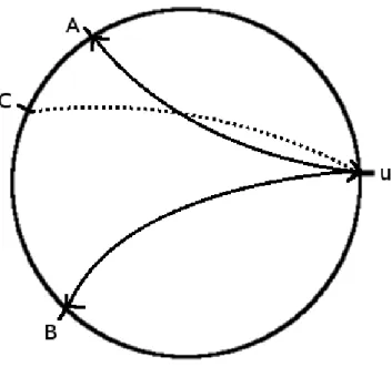
u2 (so u2 is closer from the target than u1), it means v is linked to u0, u1 and u2 so u0 should

have directly forwarded the message to u2 (see figure 7). This comes from the fact that the

ui are closer and closer from the target, so when u0 selected the neighbors of its neighbors to

which it will forward the message, it would have chose u2, not u1. This is not only working for

consecutive steps but for all the steps during the execution of the protocol. Our main problem was to get rid of the dependency of the path in the evaluation of the probabilities while keeping interesting results.

(15)

Figure 6: The node v is the kind of node we are looking for.

Figure 7: If v is linked to u0, u1 and u2 then u0 forwards to u2, not to u1

We consider two parts during the execution of the algorithm: when the message is at a distance greater than√n from the target and when it is not. When the source of the message is at a distance at least√n from the source we show that the source is able, using an intermediate node, to forward directly the message to a node at a distance lower than √n from the target

(16)

with high probability. In the other case (i.e. after the first step the message is still at a distance greater than√n from the target), we can lower bound the expected number of steps by O(ln2n) ([13]); it will be enough to reach a constant expected number of steps since that case happens with really low probability.

Then, once your are close enough of the target, you can reach a node at a distance r with a probability _r1+c1 for some fixed c, and then the expected number remaining is O(ln r) so in

average we got a constant expected number of steps.

5 Intermediate Results

5.1 Upper-bound

Lemma 1. Given a path u0, u1, .., ui, the remaining expected steps from ui to the target t is at

most O(ln2n).

Proof. Fraigniaud and Giakkoupis ([13]) have studied the routing in the same model excepted that the expected number of long-range contacts is a constant instead of O(ln n). They have shown that the expected number of steps needed to forward a message for a node u to a node t is O(ln2n) for the worst pair (u, t). Then, as having more long-range contacts, more knowledge and making the edges undirected can only improve the efficiency of the routing, O(ln2n) is also an upper-bound for our routing complexity.

5.2 First step

The first result we got is that the probability there exists a node linked to both a node u and a ball centered on a node t and of radius √_{n equals to 1 −} 1

nΩ(1), i.e. the probability that the

source forward the message to a node at a distance at most √n from the target is really high. Indeed this probability is computed assuming that no steps have been made before that is why you can only apply it from the source.

Lemma 2. Assuming that the source u0 is at a distance d ≥ √n from the target t, u1 is at a

distance at most √_{n from t with probability 1 −} 1

nO(1).

Pr(∃v, v → u0∧ v → Bt(n1/2)) = 1 −_nΩ(1)1

Proof. The probability of the existence of such a v is 1 minus the probability that none of the v is showing these properties:

Pr(∃v, v → u0∧ v → Bt(n1/2)) = 1 − Y v (1 − Pr(v → u0∧ v → Bt(n1/2))) ≥ 1 −Y v e− Pr(v→u0∧v→Bt(n1/2)) = 1 − e− P v Pr(v→u0∧v→Bt(n 1/2₎₎ = 1 − e− P v P k Pr(v→u0∧v→Bt(n1/2)|Cv=k)·Pr(Cv=k)

Now we need to compute this sum, to achieve this we need to introduce some notations: • x = dv,u

(17)

• d = du,t

With these we can obtain a formula which holds in all cases:

kXmax k=2 Pr(v → u ∧ v → Br{t} | Cv = k) · Pr(Cv = k) = kXmax k=2 Pr(v → u | Cv = k) · Pr(v → Br{t} | v → u, Cv = k) · Pr(Cv = k) ≥ kXmax k=2 Pr(v → u | Cv = k) · Pr(v → Br{t} | Cv = k − 1) · Pr(Cv = k) = kXmax k=2 (1 − (1 − _{y ln n}r )(k−1)_{)(1 − (1 −} 1 x ln n) k₎ 1 k2

We’ll have the two cases: • x · r ≤ y

• y ≤ x · r

For each of these, we have 4 cases depend-ing on v:

1. x + y = d 2. x + y = n − d 3. x = y + d 4. y = x + d

We will only consider the case y/r ≤ x and yrln n ≤ k ≤ x ln n and in that case we have:

(18)

Then we can simplify the sum : x ln n_X k=y_rln n (1 − (1 − _{y ln n}r )(k−1)_{)(1 − (1 −} 1 x ln n) k₎ 1 k2 ≥ x ln n_X k=y_rln n k xk2_{ln n} = x ln n_X k=y_rln n 1 kx ln n = Ω(ln( rx y) x ln n)

Now we will only consider the nodes in the set V1 which is enough for the probability we

want to obtain.

All the nodes v in V1 have the property that x + y = d, so we get:

∀v ∈ V1, y/r ≤ x ≤ d − 1 =⇒ _r+1d ≤ x ≤ d − 1, then: X v∈V Ω(ln( rx y ) x log n) ≥ X v∈V1 Ω(ln( rx y ) x log n) = d−1 X i=_1+rd Ω(ln( ri d−i) i log n ) ≥ d−1 X i=_1+rd Ω( ln( ri d−(_1+rd )) i log n ) = d−1 X i=_1+rd Ω(ln( (r+1)i d ) i log n ) = Ω(ln 2₍(r+1)(d−1) d ) − ln2( (r+1)( d r+1) d ) log n ) = Ω(ln 2 ((r + 1)(1 −d1)) − ln 2₍₁₎ log n ) ≥ Ω(ln 2_{((r + 1)(1 −}1 2)) log n ) ∼ Ω(ln 2_(r) log n)

(19)

Now we replace this result in the main part with r =√n: Pr(∃v, v → u0∧ v → Bt(n1/2)) = 1 − e −P v P k Pr(v→u0∧v→Bt(n1/2)|Cv=k)·Pr(Cv=k) = 1 − e−Ω(ln2(n1/2)log n ) = 1 − e−Ω(ln n) = 1 −_n_Ω(1)1

This completes the proof of that the first step reaches the ball centered on t of radius√n with high probability.

5.3 Second Step

Now we compute the probability for the second step to reach a ball of radius r centered on the target t. The computation is very similar to the previous one except we do not consider the same v: in this case we consider some v in V3 instead of V1. The intuition behind the proof is

that all the nodes are verifying x = y + d (because we are in V3) with a small d compare to x

and y (because we are at most at a distance √_{n from the target) so we have x ∼ y and then} we have some simplifications we could not have in the previous computation.

An other difference with the previous lemma is that we are not doing the first step and then we must take into account the first step, i.e. there exists a v like to both u0 and u1 and, more

importantly, no other v has a link to u0 and a node closer from the target than u1 (if not, this

node would have been selected to receive the message instead of u1).

Lemma 3. Assuming that d(u1, t) ≤√n and d(u0, t) ≥√n, the probability that the second step

reaches a ball centered on _{t of radius r is 1 −} 1

rΩ(1). Pr(∃v, v → u1∧ v → Bt(r) |6 ∃v′, v′→ u0∧ v′ → Bt(d(t, u1))) = 1 − _rΩ(1)1 Proof. Pr(∃v, v → u1∧ v → Bt(r) |6 ∃v′, v′ → u0∧ v′ → Bt(d(t, u1))) = 1 −Y v (1 − Pr(v → u1∧ v → Bt(r) | v 6→ u0∨ v 6→ Bt(d(t, u1)))) ≥ 1 − e P v P k

Pr(cv=k∧v→u1∧v→Bt(r)|v6→u0∨v6→Bt(d(t,u1)))

So we need to compute this sum, with V = {v | n2/8≤ d(v, t) ≤ n3/8} we have: X v X k Pr(cv = k ∧ v → u1∧ v → Bt(r) | v 6→ u0∨ v 6→ Bt(d(t, u1))) ≥X v∈V d ln n_X k=d ln n r Pr(cv = k ∧ v → u1∧ v → Bt(r) | v 6→ u0∨ v 6→ Bt(d(t, u1)))

(20)

So we have to simplify Pr(cv = k ∧ v → u1 ∧ v → Bt(r) | v 6→ u0 ∨ v 6→ Bt(d(t, u1)))

to be able to bound it because we can not compute this probability due to the fact that v 6→ u0∨ v 6→ Bt(d(t, u1)). Pr(cv = k ∧ v → u1∧ v → Bt(r) | v 6→ u0∨ v 6→ Bt(d(t, u1))) = = Pr(cv = k ∧ v → u1∧ v → Bt(r) ∧ (v 6→ u0∨ v 6→ Bt(d(t, u1)))) Pr(v 6→ u0∨ v 6→ Bt(d(t, u1))) ≥ Pr(cv = k ∧ v → u1∧ v → Bt(r) ∧ (v 6→ u₁ 0∨ v 6→ Bt(d(t, u1)))) ≥ Pr(cv = k ∧ v → u1∧ v → Bt(r) ∧ v 6→ u0) = Pr(cv = k ∧ v → u1∧ v → Bt(r)) · Pr(v 6→ u0 | cv = k ∧ v → u1∧ v → Bt(r)) ≥ Pr(cv = k ∧ v → u1∧ v → Bt(r)) · Pr(v 6→ u0 | cv = k) = Pr(cv = k ∧ v → u1∧ v → Bt(r)) · (1 − 1 d(v, u0) ln n )k ≥ Pr(cv = k ∧ v → u1∧ v → Bt(r)) · (1 − 1 (√_{n − n}3/8_{) ln n}) n3/8_{ln n} ∼ Pr(cv = k ∧ v → u1∧ v → Bt(r)) · (1 − 1 √ n ln n) n3/8_{ln n} ≥ Pr(cv = k ∧ v → u1∧ v → Bt(r)) · e−n −1/8 ≥ Pr(cv = k ∧ v → u1∧ v → Bt(r)) · e− 1 2 1/8 ≥ Pr(cv = k ∧ v → u1∧ v → Bt(r)) · Ω(1)

(21)

X v X k Pr(cv = k ∧ v → u1∧ v → Bt(r) | v 6→ u0∨ v 6→ Bt(d(t, u1))) ≥X v∈V d ln n_X k=d ln n_r Pr(cv = k ∧ v → u1∧ v → Bt(r)) · Ω(1) = Ω(X v∈V d ln n_X k=d ln n_r Pr(cv = k ∧ v → u1∧ v → Bt(r))) = Ω(X v∈V d ln n_X k=d ln n_r 1 k2 · k d(v, t) ln n· 1) = Ω(X v∈V ln r d(v, t) ln n) = Ω(ln r ln n · ln(n 1/8₎₎ = Ω(ln r) So we get: Pr(∃v, v → u1∧ v → Bt(r) |6 ∃v′, v′ → u0∧ v′ → Bt(d(t, u1))) = 1 −Y v (1 − Pr(v → u1∧ v → Bt(r) | v 6→ u0∨ v 6→ Bt(d(t, u1)))) ≥ 1 − e P v P k

Pr(cv=k∧v→u1∧v→Bt(r)|v6→u0∨v6→Bt(d(t,u1)))

= 1 − e−Ω(ln r)

= 1 − 1 rΩ(1)

This completes the proof that, given the path u0u1 with d(u0, t) ≥√n and d(u1, t) ≤√n, we

have d(u2, t) ≤ r with probability 1 − _rΩ(1)1 .

5.4 Last step

Now we try to bound the probability that the message reaches a ball centered on the target of radius r given a path of length i. We do not need a bound really big so we can afford some simplification to make the computation easy.

Lemma 4. The probability that exists a node v, both link to ui and a ball of radius r centered

ont, given a path u0..ui isΩ(r_i), in other words, given such a path of length i + 1, the probability

that the next step reaches a node at a distance lower than r from the target is Ω(r_i). Pr(∃v, v → ui∧ v → Bt(r) | u0u1..ui) = Ω(r_i)

(22)

Proof. Pr(∃v, v → ui∧ v → Bt(r) | u0u1..ui) = 1 − Y v (1 − Pr(v → ui∧ v → Bt(r) | u0u1..ui−1)) ≥ 1 −Y v

e− Pr(v→ui∧v→Bt(r)|u0u1..ui)

≥ 1 − e−

P

v Pr(v→ui∧v→Bt(r)|u0u1..ui)

≥ 1 − e−

P

v

P

k

Pr(v→ui∧v→Bt(r)∧Cv=k|u0u1..ui)

So as usual, we need to compute the sum, so we need to simplify Pr(v → ui∧v → Bt(r)∧Cv = k |

u0u1..ui) to get rid of the dependency on the path. The fact that the path is u0..ui means that

any v we consider as a candidate to forward the message must not have links to the couples (uj,

Bt(d(t, uj+1))) for all j because if there were such an v linked to a couple (uj, Bt(d(t, uj+1))),

instead of forwarding to uj+1, uj would have transferred the message directly to Bt(d(t, uj+1))

via v. Pr(v → ui∧ v → Bt(r) ∧ Cv = k | u0u1..ui) = Pr(v → ui∧ v → Bt(r) ∧ Cv = k) · Pr(V_j_{(v 6→ u}j∨ v 6→ Bt(d(uj+1, t))) | v → ui∧ v → Bt(r) ∧ Cv = k) Pr(V_j_{(v 6→ u}j ∨ v 6→ Bt(d(uj+1, t)))) ≥ Pr(v → ui∧ v → Bt(r) ∧ Cv = k) · Pr(V_j_{(v 6→ u}j∨ v 6→ Bt(d(uj+1, t))) | v → ui∧ v → Bt(r) ∧ Cv = k) 1 ≥ Pr(v → ui∧ v → Bt(r) ∧ Cv = k) · Pr( ^ j (v 6→ uj) | v → ui∧ v → Bt(r) ∧ Cv= k) ≥ Pr(v → ui∧ v → Bt(r) ∧ Cv = k) · Pr( ^ j (v 6→ uj) | Cv = k) ≥ Pr(v → ui∧ v → Bt(r) ∧ Cv = k) · Θ(1) = Ω(Pr(v → ui∧ v → Bt(r) ∧ Cv = k))

(23)

X v Pr(v → ui∧ v → Bt(r) | u0u1..ui) = X v X k Pr(v → ui∧ v → Bt(r) ∧ Cv = k | u0u1..ui) ≥X v d(v,ui) ln n i X k=1 Pr(v → ui∧ v → Bt(r) ∧ Cv = k | u0u1..ui) ≥X v d(v,ui) ln n i X k=1 Ω(Pr(v → ui∧ v → Bt(r) ∧ Cv = k)) =X v d(v,ui) ln n i X k=1 Ω( 1 k2 · k · r d(v, t) ln n· k d(v, ui) ln n ) =X v Ω( r d(v, t)· 1 i ln n) = Ω(r i) So we have: Pr(∃v, v → ui∧ v → t | u0u1..ui−1) ≥ 1 − e −P v

Pr(v→ui∧v→t|u0u1..ui−1)

≥ 1 − e−Ω(ri)

≥ 1 − (1 − 1₂ · Ωr_i)) = Ω(r

i) The last two lines use the fact that e−x_{≤ 1 −}x

2 for 0 ≤ x ≤ 1.

With this we have proven that Pr(∃v, v → ui∧ v → t | u0u1..ui−1) = Ω(r_i).

5.5 Expected number of steps from u₂

Now we compute the number of remaining steps X(u2), using the previous lemma, needed to

forward the message from u2 to a constant distance r from the target.

Lemma 5. Exists a value r for which the expected number of steps, given the path u0, u1, u2

with d(u2, t) = d is O(ln d).

E(X(u2)) = O(ln d)

Proof. _{Let E}i the fact that the message reaches ball of radius r centered on the target in exactly

i steps. The probability that X(u2) is greater or equal to some constant j is the probability that the message has not reached the target in less than j + 2 steps, which can be expressed by

(24)

the Ei. E(X(u2)) = d−r X j=1 Pr(X(u2) ≥ j) ≤ d X j=1 Pr(X(u2) ≥ j) = d X j=1 Pr( j−1_^ i=3 ¬Ei) = d X j=1 Pr(¬E3) · Pr( j−1_^ i=2 ¬Ei| ¬E3) = d X j=1 j−1 Y i=3 Pr(¬Ei| ^ p≤i ¬Ep) = d X j=1 j−1 Y i=3 (1 − Ω(r_i)) = (1 − Ω(r₃)) + (1 − Ω(r₃)) · (1 − Ω(r₄)) + .. + (1 − Ω(r₃)) · .. · (1 − Ω(_dr)) ≤ (1 − c · r₃ ) + (1 − c · r₃ ) · (1 − c · r₄ ) + .. + (1 − c · r₃ ) · .. · (1 −c · r_d )

For some constant c.

Here we have two cases: or c ≥ 1 and then r = 1 is enough, else we need r ≥ 1c. In both cases

we have : ≤ (1 − 1₃) + (1 − 1₃) · (1 −1₄) + .. + (1 − 1₃) · .. · (1 −_d1) = 2 3 + 2 3 · 3 4+ .. + 2 3· .. · d − 1 d = 2 · (1₃+ 1 3· 3 4 + .. + 1 3 · .. · d − 1 d ) = 2 · (1₃+ 1 4+ .. + 1 d) ≤ O(1₁+ 1 2+ .. + 1 d) = O(ln d)

So we have proved that there exists a value r for which the expected number of steps, given the path u0, u1, u2 with d(u2, t) = d, to reach a ball of radius r centered on t is O(ln d).

(25)

6 Proof of the result

In this section we will prove that the routing protocol reaches the target in a O(1) expected number of step.

First we have to consider the case that the source u0 of the message is at a distance d(u0, t) ≥

√

n from the target t, from that case we will have two subcases : if the message, after two steps, is close enough of the target or not. The other case is when the source u0 is at a distance

d(u0, t) ≤√n from t.

If we have d(u0, t) ≥√n, the probability that message fails to reach a distance lower that

√

n in one step is _nΩ(1)1 from the observation 1. So in that case, from the lemma 1, the expected

number of steps to reach the target is O(ln2n). In the other case, which happens with the probability 1 −_nΩ(1)1 , we have to compute the expected number E of remaining steps to reach t:

E =X

r≥1

Pr(d(u2, t) = r) · E(length of the path from u2 to t | u0, u1, u2)

Thanks to the previous lemma, we know that there exists a constant value d for which E(length of the path from u2 to Bt(d) | u0, u1, u2, d(u2, t) = r) is O(ln r) and we have such a

(26)

E =X

r≥1

Pr(d(u2, t) = r) · E(length of the path from u2 to t | u0, u1, u2)

E ≤ d +X

r≥1

Pr(d(u2, t) = r) · E(length of the path from u2 to Bt(d) | u0, u1, u2)

= d +X

r≥2

(Pr(u2 ≤ r) − Pr(u2 ≤ r − 1)) · O(ln r) from lemma 5

= d +X

r≥2

((1 − _r1_ǫ) − (1 − 1

(r − 1)ǫ)) · O(ln r) from lemma 3

= d +X r≥2 ( 1 (r − 1)ǫ − 1 rǫ) · O(ln r) = d +X r≥2 (r ǫ_{− (r − 1)}ǫ (r · (r − 1))ǫ) · O(ln r) = d +X r≥2 (r ǫ_{· (1 − (1 −}1 r)ǫ) (r · (r − 1))ǫ ) · O(ln r) = d +X r≥2 ((1 − (1 − 1 r)ǫ (r − 1)ǫ ) · O(ln r) ≤ d +X r≥2 ( O( ǫ r) (r − 1)ǫ) · O(ln r) = d +X r≥2 O( ǫ r · (r − 1)ǫ) · O(ln r) ∼ d +X r≥2 O( ǫ r1+ǫ) · O(ln r) ≤ d +X r≥2 O( 1 r1+ǫ) · O(ln r) = d +X r≥2 O(ln r r1+ǫ) ≤ d +X r≥2 O( 1 r1+ǫ′) with ǫ ′_{< ǫ} ≤ O(d + 1 − 1 n2+ǫ′2 ) = O(1)

So for the entire routing we get 2 + O(1) = O(1) with probability 1 −_nΩ(1)1 and O(ln2n) with

probability _nΩ(1)1 so the expected number of steps when d(u0, t) ≥

√ n is:

(27)

O(1) · (1 −_nΩ(1)1 ) + O(ln2n) · _nΩ(1)1 = O(1).

In the case d(u0, t) ≤ √n we have to adapt the probabilities: the probability of that first

step (which corresponds to the second in the previous case) will reach a ball of radius r centered on t is still 1 −_rΩ(1)1 , and then we can use the other lemma since the only things that differs is

the length of the path traveled which is decreased by 1. Pr(∃v, v → u1∧ v → Bt(r)) = 1 − Y v (1 − Pr(v → u1∧ v → Bt(r))) ≥ 1 − e P v P k Pr(cv=k∧v→u1∧v→Bt(r))

Then the end of the computation is the same as in the proof of the lemma 3 so we also get that the step reaches a ball of radius r centered in t with probability 1 − _rΩ(1)1 .

The lemma 4 remains the same and we just have to adapt the proof of the lemma 5: we have one term more in the sum, we just need the term 1 to get the harmonic sum so instead of adding both 1 and 1/2 we just add 1 to get our O(ln d) result.

Then by the same argument as before we get that the expected number of steps for a source at a distance at most√n from a target to send a message to this target is O(1).

So, in any case, our protocol performs a routing between any source-target pair in O(1) expected number of steps.

7 Conclusion and future work

Our aim was to improve Kleinberg’s ring-based model by using two ideas (having a variable number of long-range contacts and having mode knowledge about the network) already used but not together.

So by taking the 1-dimensional grid graph with a variant number of nodes defined by Fraig-niaud and Giakkoupis ([13]), increasing the expected number of long-range contact to O(ln n) and adding knowledge we achieve a routing in O(1) steps which is optimal for the complexity of a routing algorithm. The fact that we get an optimal complexity also allows us to conclude that additional look-ahead is useless as it was found by Manku, Naor and Wieder in their study over original Kleinberg’s model ([23]).

It would be interesting to remove the extra-knowledge of the nodes and try to simulate it: instead of already knowing the neighbors of your neighbors, you send a message to all your neighbors to ask them about their closest neighbor from the target. By making the edges bidirectional we double the number of edges, so the average number of neighbor of the nodes remains O(ln n) then it would be tempting to say that this protocol allows to find the short paths by sending O(ln n) messages since every node of the O(1) nodes of the path asks all their neighbors. Unfortunately that is wrong because thought the average degree of a random node is O(ln n) that is not the case for the one of the path because in average, the average number of friends of your neighbors is higher than yours. This phenomenon is called the ”friendship paradox” and is explained ([9]) by the fact when you compute the average number of friends you will count the nodes with a lot of friends once for every friends of its! So node with high degree have an huge influence on the average value compare to the one with few neighbors.

Due to a matter of time we did not study a protocol based on homophily and degree disparity as we intended to. The idea is to limit the knowledge of the nodes concerning their neighborhood: instead of knowing the neighbors of their neighbors, the nodes only know the degree of their neighbors. The underlying algorithm to this knowledge, i.e. not forward to the node which is the

(28)

closest nor the one with the more neighbors but to the one which is the more likely to forward to a node close to the target (this probability depends on both the degree and the distance from the target), have been studied by Simsek and Jensen ([30]) and was very effective. In our case we should have forwarded the message to the node v which maximizes 1 − (1 −d(v,t) ln n1 )Cv, i.e.

which maximizes the probability of having at least one edge directed to the target. It depends on both the distance of the node from the target and the degree Cv of the node v.

Computing the diameter is also in the continuation of this internship: the diameter of a network is the longest of the shortest path there are in a network. To compute it you need select, for every pair of nodes, the shortest path between them; then, now you have one path for every pair of nodes, you select the longest one and its size is the diameter of the network. The diameter is the time needed for a message to be forwarded from a source to a target using the shortest path, in the worst case. The shortest is it, the best is it for routing assuming you are able to find the right path. It is also interesting for computing a average efficiency for the worst pair; in our case we only compute the average efficiency for any pair.

Also it would be interesting to generalize these results to the l-dimensional grid as it was done with most of all the works done on the grid-based networks. As with the other results, we could expect a O(1) expected number of steps with good distributions. Then the study of the influence on the distribution on the efficiency of the algorithm and on the diameter should be a good continuation of this work.

(29)

8 References

[1] L. A. Adamic, R. M. Lukose, A. R. Puniyani, and B. A. Huberman. Search in power-law networks. Physical Review E, 64, 2001.

[2] R. Albert and A.-L. Barab´asi. Statistical mechanics of complex networks. Reviews of Mod-erna Physics, 74(1):47–97, 2002.

[3] A.-L. Barab´asi and R. Albert. Emergence of Scaling in Random Networks, Science 286, 509 (1999).

[4] D. Coppersmith, D. Gamarnik, and M. Sviridenko. The diameter of a long range percola-tion graph. In Proceedings of the 13th Annual ACM-SIAM Symposium on Discrete Algorithms (SODA), pages 329-337, 2002.

[5] M. Dietzfelbinger, J. Rowe, I. Wegener, and P. Woefel. Tight bounds for blind search on the integers. In Proceedings of the 25th International Symposium on Theoretical Aspects of Computer Science (STACS), pages 241-252, 2008.

[6] Martin Dietzfelbinger and Philipp Woelfel. Tight lower bounds for greedy routing in uni-form small world rings. In Proceedings of the 41nd ACM Symposium on Theory of Computing (STOC), pages 591–600, 2009.

[7] Peter Sheridan Dodds, Muhamad Roby, and Duncan J Watts. An experimental study of search in global social networks. Science, 301:827–829, 2003.

[8] S. N. Dorogovtsev and J. F. F. Mendes. Evolution of networks: From biological networks to the Internet and WWW. Oxford University Press, 2003.

[9] Scott L. Feld. Why Your Friends Have More Friends Than You Do. The American Journal of Sociology, Vol. 96, No. 6, pp. 1464-1477, 1991.

[10] P. Fraigniaud, C. Gavoille, and C. Paul. Eclecticism shrinks even small worlds. In Pro-ceedings of the 23rd ACM Symposium on Principles of Distributed Computing (PODC), pages 169-178, 2004.

[11] Pierre Fraigniaud and George Giakkoupis. The effect of power-law degrees on the naviga-bility of small worlds. In Proceedings of the 28nd ACM Symposium on Principles of Distributed Computing (PODC), pages 240–249, 2009.

[12] Pierre Fraigniaud and George Giakkoupis. On the searchability of small-world networks with arbitrary underlying structure. In Proceedings of the 42nd ACM Symposium on Theory of Computing (STOC), pages 389–398, June 6–8 2010.

[13] Pierre Fraigniaud and George Giakkoupis. Greedy Routing in Small-World Networks with Power-Law Degrees. Preprint.

[14] George Giakkoupis and Nicolas Schabanel. Optimal path search in small worlds: dimension matters. In Proceedings of the 43nd ACM Symposium on Theory of Computing (STOC), pages 393–402, 2011.

(30)

Physical Review E, 65:027103, 2002.

[16] Jon Kleinberg. The small-world phenomenon: an algorithm perspective. In Proceedings of the 32nd ACM Symposium on Theory of Computing (STOC), pages 163–170, 2000.

[17] J. Kleinberg. Navigation in a small world. Nature, 406:845, 2000.

[18] J. Kleinberg. Small-world phenomena and the dynamics of information. In Advances in Neural Information Processing Systems (NIPS) 14, pages 431–438, 2001.

[19] Jon Kleinberg. Complex networks and decentralized search algorithms. In International Congress of Mathematicians (ICM), pages 1019–1044, 2006.

[20] S. Lattanzi, A. Panconesi, and D. Sivakumar. Milgram-routing in social networks. In Proceedings of the 20th ACM International Conference on World Wide Web (WWW), pages 725-734, 2011.

[21] E. Lebhar and N. Schabanel. Almost optimal decentralized routing in long-range contact networks. In proceedings of the 31st International Colloquium on Automata, Languages, and Programming (ICALP), pages 894-905, 2004.

[22] D. Liben-Nowell, J.Novak, R. Kumar, P. Raghavan, and A. Tomkins. Geographic routing in social networks. In Proceedings of the National Academy of Sciences of th USA, 102(33):11623-11628, 2005.

[23] Gurmeet Singh Manku, Moni Naor, and Udi Wieder. Know thy neighbor’s neighbor: the power of lookahead in randomized P2P networks. In Proceedings of the 36nd ACM Symposium on Theory of Computing (STOC), pages 54–63, 2004.

[24] Gurmeet Singh Manku. Routing networks for distributed hash tables. In Proceedings of the 22nd ACM Symposium on Principles of Distributed Computing (PODC), pages 133–142, July 2003.

[25] C. Martel and V. Nguyen. Analyzing Kleinberg’s (and other) small-world models. In Pro-ceedings of the 23rd ACM Symposium on Principles of Distributed Computing (PODC), pages 179–188, 2004.

[26] C. Martel and V. Nguyen. Analyzing and characterizing small-world graphs. In Proceedings of the 16th Annual ACM-SIAM Symposium on Discrete Algorithms (SODA), pages 311–320, 2005.

[27] Stanley Milgram. The small world problem. Psychology Today, 1:60–67, 1967.

[28] M. E. J. Newman. The structure and function of complex networks. Society for Industrial and Applied Mathematics (SIAM) Review, 45(2):167–256, 2003.

[29] N. Sarshar, P. O. Boykin, and V. P. Roychowdhury. Percolation search in power law net-works : Making unstructured peer-to-peer netnet-works scalable. In Proceedings of the 4th IEEE International Conference on Peer-to-Peer Computing (P2P), pages 2-9, 2004.

[30] Ozgur Simsek and David Jensen. Decentralized search in networks using homophily and degree disparity. In International Joint Conferences on Artificial Intelligence (IJCAI), pages

(31)

304–310, 2005.

[31] Duncan J. Watts, Steven H. Strogatz. Collective dynamics of ’small-world’ networks. Na-ture 393, pp.440-442, 1998.