HAL Id: hal-00298273
https://hal.archives-ouvertes.fr/hal-00298273
Submitted on 21 Oct 2005
HAL is a multi-disciplinary open access
archive for the deposit and dissemination of
sci-entific research documents, whether they are
pub-lished or not. The documents may come from
teaching and research institutions in France or
abroad, or from public or private research centers.
L’archive ouverte pluridisciplinaire HAL, est
destinée au dépôt et à la diffusion de documents
scientifiques de niveau recherche, publiés ou non,
émanant des établissements d’enseignement et de
recherche français ou étrangers, des laboratoires
publics ou privés.
the Tropical Atlantic Ocean
A. C. V. Caltabiano, I. S. Robinson, L. P. Pezzi
To cite this version:
A. C. V. Caltabiano, I. S. Robinson, L. P. Pezzi. Multi-year satellite observations of instability waves
in the Tropical Atlantic Ocean. Ocean Science, European Geosciences Union, 2005, 1 (2), pp.97-112.
�hal-00298273�
www.ocean-science.net/os/1/97/ SRef-ID: 1812-0792/os/2005-1-97 European Geosciences Union
Ocean Science
Multi-year satellite observations of instability waves in the Tropical
Atlantic Ocean
A. C. V. Caltabiano1, I. S. Robinson2, and L. P. Pezzi3
1International CLIVAR Project Office, National Oceanography Centre, European Way, Southampton, SO14 3ZH, UK 2School of Ocean and Earth Science, National Oceanography Centre, European Way, Southampton, SO14 3ZH, UK 3Centro de Previs˜ao de Tempo e Estudos Clim´aticos (CPTEC/INPE), Rod Presidente Dutra, Cachoeira Paulista, SP,
12630-000, Brazil
Received: 22 December 2004 – Published in Ocean Science Discussions: 21 January 2005 Revised: 1 August 2005 – Accepted: 4 October 2005 – Published: 21 October 2005
Abstract. Instability waves in the tropical Atlantic Ocean are
analysed by microwave satellite-based data spanning from 1998 to 2001. This is the first multi-year observational study of the sea surface temperature (SST) signature of the Tropical Instability Waves (TIW) in the region. SST data were used to show that the waves spectral characteristics vary from year-to-year. They also vary on each latitude north of the equa-tor, with the region of 1◦N, 15◦W concentrating the largest variability when the time series is averaged along the years. Analyses of wind components show that meridional winds are more affected near the equator and 1◦N, while zonal winds are more affected further north at around 3◦N and 4◦N. Concurrent observations of SST, wind, atmospheric water vapour, liquid cloud water, precipitation rates and wind were used to suggest the possible influence of these waves on the Intertropical Convergence Zone (ITCZ). It seems that these instabilities have a large impact on the ITCZ due to its proximity of the equator, compared to its Pacific counter-part, and the geography of the tropical Atlantic basin. These analyses also suggest that the air-sea coupling mechanism suggested by Wallace et al. (1989) can also be applied to the tropical Atlantic region.
1 Introduction
Cusp-shaped frontal waves have been observed very often in the tropical Pacific region, more developed north of the equator. Such waves, known as Tropical Instability Waves (TIWs), were first studied by Legeckis (1977) using radiome-ters on geostationary satellites. Since then, they have been extensively studied by other orbital infrared sensors (Allen et al., 1995), in situ data (Halpern et al., 1988; Hayes et al., 1989) and ocean models (Philander et al., 1986; Masina
Correspondence to: A. C. V. Caltabiano
and Philander, 1999). Most recently, several studies have been performed using SST data retrieved from an orbital microwave sensor (Chelton et al., 2000; Hashizume et al., 2001).
The phenomenon of TIWs has generally been attributed to intense latitudinal shears between the various compo-nents of the equatorial current system that cause the currents to become unstable (Philander, 1978; Cox, 1980). Other observational studies confirm that the TIWs modify the mean oceanic currents by reducing the shears between them (Hansen and Paul, 1984; Weisberg, 1984). The instabilities cause large perturbations of the SST front between the colder upwelling water of the Pacific equatorial cold tongue and the warmer water to the north (Flament et al., 1996; Kennan and Flament, 2000). Qiao and Weisberg (1995) estimated that TIWs in the equatorial Pacific propagate westwards with pe-riods of 20–40 days, wavelengths of 1000–2000 km and a phase speed of ∼0.5 ms−1. In spite of oceanic origin, TIWs variability can project onto the atmosphere, affecting the for-mation of cloud (Deser et al., 1993; Hashizume et al., 2001), changing the heat flux (Thum et al., 2002), and causing wind variations (Hayes et al., 1989; Chelton et al., 2001; Liu et al., 2000; Hashizume et al., 2002) with similar 20–30-day peri-odicities.
TIWs-induced oceanic eddy heat flux towards the equa-tor has been shown to be comparable to the Ekman heat flux away from the equator and the large-scale net air-sea heat flux over the tropical Pacific (Wang and McPhaden, 1999). Also, using a moored array dataset, Wang and Weisberg (2001) showed that the vertical and zonal eddy temperature fluxes are much smaller than the meridional eddy tempera-ture flux, although the heat flux in the central Pacific is dom-inated by mean heat flux. Nevertheless, TIWs are an impor-tant component of the large-scale heat balance of the equato-rial cold tongue. These modifications of heat flux induce per-turbations of the surface wind stress field that are controlled by perturbations of the underlying SST field.
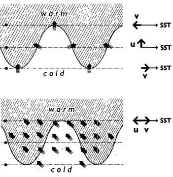
Fig. 1. Schematic representation of perturbation of the surface wind
field (U = zonal wind, V = meridional wind) associated with a TIW, following the hypothesis suggested by Lindzen and Nigam (1987) (top panel) and Wallace et al. (1989) (bottom panel). Arrows in the figure represent wind. Modified from Hayes et al. (1989).
On the other hand, analyzing the TIWs-ABL1 coupling, the open question has been for a while whether these TIWs-induced perturbations of the wind field have a significant feedback onto the ocean circulation. Pezzi et al. (2004) in-vestigated if this feedback occurs in the tropical Pacific. The authors showed that the wind perturbations apparently have a negative feedback that tends to reduce the SST and merid-ional velocity signatures of TIWs. This, in turn, reduces the equatorward eddy heat flux associated with TIWs, thereby resulting in intensified cooling of the equatorial cold tongue. This negative feedback has potential far-reaching implica-tions about the role of TIWs in climate variability.
Hayes et al. (1989) investigated the relationship between TIWs-induced perturbations of SST and surface wind. They found a strong correlation between the meridional gradient of SST and the meridional gradient of the northward wind component. The importance of SST-induced modifications of atmospheric stability has been further investigated from satellite observations of the geographical distribution of low-level cloudiness in relation to the SST signatures of TIWs (Deser et al., 1993). That study proposed that as the south-easterly trades blow across the meandering equatorial front, thermal convection may occur over the warm sector and help form clouds.
There are two main hypotheses concerning the relation be-tween SST and surface winds over the tropical oceans. In
1Atmospheric Boundary Layer
the first hypothesis, SST couples with sea level pressure and changes the wind (Lindzen and Nigam, 1987). Lower and higher pressures are found over warmer and cooler water, re-spectively. As zonal winds move down the pressure or up the temperature gradient, the zonal winds always remain 90◦ out of phase with SST and in phase with the zonal gradient of SST. The meridional component is accelerated northward at both the crest (north) and trough (south) of the waves. At the crest, the ocean is cold and meridional wind is 180◦out of phase with SST. At the trough, the ocean is warm and meridional wind is in phase with SST. The strongest wind should be found at the highest pressure or SST gradient. In the second hypothesis (Wallace et al., 1989), SST is coupled with wind through the stability (density stratification) change in the atmospheric boundary layer. Over warm water, air is more buoyant, mixing increases, and wind shear is reduced in the boundary layer. Surface winds increase as consequence. The opposite is true over cold water.
The two hypotheses that could explain the perturbation of the surface wind speed by a westward propagating SST field associated with TIWs are summarised in Fig. 1. The top panel assumes principal forcing is through the hydrostatic influence on the atmospheric sea-level pressure (SLP) as dis-cussed in Lindzen and Nigam (1987). Warm SST is associ-ated with low SLP, cool water with high SLP. Near the equa-tor surface winds tend to flow down the SLP gradient. As summarised by the diagram in Fig. 1, zonal wind (U) pertur-bations are 90◦out of phase with the SST while meridional wind (V) changes tend to be either in phase or 180◦out of phase depending upon the latitude. Bottom panel assumes that the principal coupling of SST and wind is through mod-ification of the boundary layer shear as discussed in Wallace et al. (1989). In this case surface winds are stronger over warm SST. For the southeasterly winds shown, zonal winds are 180◦out of phase with SST perturbations and meridional winds are in phase with them.
More recently, a modelling study by Small et al. (2003) provided evidence of the relative importance of pressure forcing. They suggested that SLP anomalies are not collo-cated with SST anomalies in the particular case of TIWs. Their model results indicate that the mechanism suggested by Wallace et al. (1989) may be unreliable because of the thermal and moisture advection by the mean wind. Sea level pressure is lagged downstream of the SST anomalies, and the authors show that pressure driving is dominant and sufficient to cause pressure driven winds to be in phase with SST.
Most of the studies cited above were performed using data from the tropical Pacific. TIWs in the tropical Atlantic (Fig. 2), most probably due to the lack of in situ data, are subjects of only a few studies. Duing et al. (1975) were the first to notice TIWs in the tropical Atlantic during the GATE programme. Weisberg and Weingartner (1988), using cur-rent meter data from surface moorings deployed during the SEQUAL/FOCAL programs, described the TIWs properties in the tropical Atlantic. They found a packet of waves with
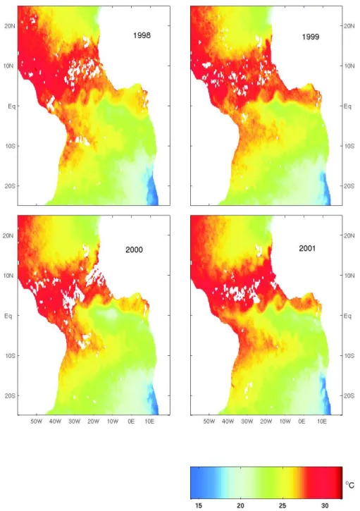
Fig. 2. Series of 3-day mean TMI SST composites showing examples of TIWs for the years 1998, 1999, 2000 and 2001.
central periodicity of 25 days, zonal wavelength around 1100 km and phase speed of 0.5 ms−1.
Weisberg and Weingartner (1988) also found that, thermo-dynamically, the waves affect the southward heat transport during the period when the North Equatorial Countercurrent (NECC) is most rapidly gaining heat, suggesting that the waves act to regulate the heat stored in the NECC. Also, the Reynolds’ heat flux convergence upon the equator appears to halt the upwelling induced cooling and to increase SST. Dy-namically, the waves decelerate the South Equatorial Current
(SEC) north of the equator and reduce its shear. This occurs simultaneously with deceleration of the SEC by the basin-wide adjustment of the zonal pressure gradient (ZPG). The seasonal modulation of the waves is therefore a consequence of both the ZPG response to seasonally varying wind stress as well as the instability itself since both are stabilizing.
Hashizume et al. (2001) used satellite data to describe the variability of several parameters associated with the TIWs in the tropical Pacific and tropical Atlantic basins. They found that, in the Atlantic, the TIWs signals are strongly trapped
near the equator, with a wavelength of about 9◦in longitude,
slightly shorter than the Pacific ones. Also, in the Atlantic, the TIWs have a rapid development/decay, unlike the Pa-cific counterpart which has much more gradual development. This is presumably because the Atlantic is more strongly in-fluenced by its neighbouring continents. Nevertheless, the authors used only a very short time series of the TMI and QuikSCAT dataset, which prevented any interannual com-parison.
Recently Menkes et al. (2002) showed the effects of tropi-cal vortices in the Atlantic Ocean, which are associated with TIWs, and their influence on phytoplankton, zooplankton and small pelagic fish communities. Biologically rich in nutrients and cold equatorial waters are advected northward and downward to form sharp fronts visible in all tracers and trophic levels. The equatorward recirculation experiences upwelling at depth, with the pycnocline and ecosystem pro-gressively moving toward the surface to reconnect with the equatorial water mass. The observations thus indicate that it is a fully three-dimensional circulation that dominates the distribution of physical and biological tracers in the presence of tropical instabilities and maintains the cusp-like shapes of temperature and chlorophyll observed from space.
There are still some questions that remain open about TIWs in the Atlantic: do TIWs spectral characteristics in the tropical Atlantic vary from year to year? Where are they more active? Also, the hypotheses of ocean-atmosphere cou-pling on the properties of TIWs have not been fully discussed for the tropical Atlantic. As the study of TIWs in the Atlantic is still an active field of investigation, this paper will focus on the SST signature of the TIWs, and explore the temporal and spatial variabilities associated with these waves in the trop-ical Atlantic. Moreover, it will investigate multi-year vari-ations of the TIWs in the Atlantic basin using high-quality satellite data. These datasets also allow an assessment of the co-variability of geophysical fields measured by satellite and that can be affected by the instability waves. Therefore, we aim to contribute to the understanding of this topic in the re-gion.
2 Datasets and methods
In this study, two satellite sensors were used: the Tropi-cal Rainfall Measuring Mission Microwave Imager (TMI) and the QuikSCAT Seawinds. Both datasets were pro-cessed and made available by Remote Sensing Systems (http://www.ssmi.com), gridded at a 0.25◦×0.25◦. TMI data
used in this work is the TMI product Version 2, spanning from Jan 1998 to Dec 2001. The SeaWinds data is the prod-uct Version 2, spanning from June 1999 to Dec 2001.
The TMI (Kummerow et al., 1998) is a multi-channel dual-polarized passive microwave radiometer, which provides an unprecedented view of SST. It utilizes nine channels with operating frequencies of 10.65 GHz, 19.35 GHz, 21.3 GHz,
37 GHz, and 85.5 GHz. Its lowest frequency channel pene-trates non-rain clouds with little attenuation, giving a clear view of the sea surface under all weather conditions except rain. This is a distinct advantage over the traditional infrared SST observations that require a cloud-free field of view. Fur-thermore, at this frequency, microwave retrievals are not af-fected by aerosols and are insensitive to atmospheric water vapour, making it possible to produce a very reliable SST time series for climate studies. The dataset has been vali-dated by Gentemann et al. (2004), by comparing them with moored buoy measurements, which showed a good accuracy of TMI SST retrievals. Moreover, TMI is capable of retriev-ing other geophysical variables that will also be used in this work: atmospheric water vapour (VAP), liquid cloud water (CLD) and precipitation rates (RAIN), in addition to SST. For these analyses, daily maps were averaged in 3-day mean composites, spanning four years (1998–2001). The only pro-cessing needed to be applied to this dataset was to fill any gaps due to strong rain, using a 3×3 window mean interpo-lation.
The primary sensor onboard of QuikSCAT satellite is the microwave scatterometer SeaWinds, which operates at Ku-band (13.4 GHz). Surface wind speed measurements are made for a range of 3 to 20 ms−1, with an accu-racy of 2 ms−1, and direction measurements have an accu-racy of 20◦. For a question of consistency with most of the literature, the SeaWinds dataset will be referred in this work as QuikSCAT data. The data processing scheme uses contemporaneous microwave radiometer measurements for rain flagging (F13 SSMI, F14 SSMI, F15 SSMI, and TMI) and sea ice detection (all the previous except TMI). The QuikSCAT dataset contains four rain flags, well designed for combination into a single rain flag. For the best quality data from QuikSCAT, all cells for which the scatterometer rain flag is set have been removed to avoid rain contamination to the data.
In order to isolate the TIWs variability from other strong temperature signals found in the region, such as the seasonal cycle, a filtering scheme was used. The filter applied was a westward-only 2-D finite impulse response (FIR) filter, fol-lowing the method employed by Cipollini et al. (2001). The filter is designed using prior knowledge of the approximate range of the period and wavelength of the waves. This in-formation is set as input and restricts the filter output to a particular region of the frequency-wavelength spectrum. It has a 1/4 length size sample kernel, with a bandpass of 5◦to
20◦in the longitude and 20 to 40 days in time. We used this
filter to derive the anomaly fields of SST, integrated water vapour (VAP), rain and cloud liquid water (CLD) from TMI (1998 to 2001), and zonal (U) and meridional (V) wind from QuickSCAT (2000 and 2001).
Once the data is filtered, the Radon Transform (RT) (Deans, 1983) technique is applied to estimate the propaga-tion characteristics of the TIWs. The RT has been success-fully used in determining waves propagation characteristics
Equator 40W 20W 0E 2002 2001 2000 1999 1998 1N 40W 20W 0E 2N 40W 20W 0E 3N 40W 20W 0E 22 24 26 28 30 32 34 4N 40W 20W 0E
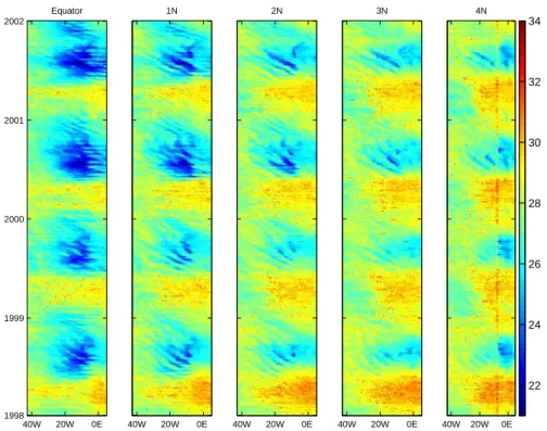
Fig. 3. Time-longitude plots of TMI SST data at the equator, 1◦N, 2◦N, 3◦N, 4◦N. SST is in◦C.
observed in altimeter dataset (Polito and Cornillon, 1997), and only more recently in SST (Hill et al., 2000) and ocean colour data (Cipollini et al., 2001).
As we aim to investigate the co-variability of the geophys-ical fields measured by the satellite sensors in the tropgeophys-ical Atlantic, their anomaly fields were used to map the spatial structure of the coupled TIWs. A linear regression technique, summarised below and successfully used by Hashizume et al. (2001), was applied. It searches for a linear relation between one of the filtered atmospheric fields F(x,y,t) and filtered SST at a reference station T(t):
F = aT (1)
A least squares fitting leads to the regression coefficient,
a(x, y) = N X n=1 F (x, y, tn)T (tn)/ N X n=1 T2(tn) (2)
Because SST varies on much shorter timescales than other variables, the atmospheric fields will be regressed onto the SST time series on a chosen grid point, which is defined as the grid point with maximum SST variability. From the re-sults achieved in Sect. 3.1, this point has been defined as be-ing at 1◦N and 15◦W.
3 Results
3.1 Temperature fields
Figure 3 presents the time-longitude plots of SST derived from TMI for five different latitudes (equator, 1◦N, 2◦N, 3◦N and 4◦N) in the tropical Atlantic. Even without any filtering, it is possible to see westward propagating features in the last six month of each of the years, when the Atlantic cold tongue is well developed. The variation with year and latitude of the TIWs signatures can be clearly observed in the plots. In 1999, the cold tongue was not very well de-veloped in which case the more energetic region of TIWs is observed around 1◦N and after July. However, in 2000, the
cold tongue appears well developed. The regions where the high gradients and high instability can be observed are dis-placed somewhat further north (2◦N) when compared to the previous years. Also, the cold tongue starts to develop ear-lier, in late May.
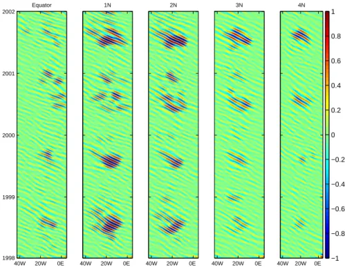
Figure 4 shows the SST time-longitude filtered fields based on the same data as Fig. 3. It shows that the filter effectively removes any signal propagating to the east and other variability signals, including the cold tongue itself. The results suggest that the largest variability of the TIWs in the tropical Atlantic can be found at 1◦N and 2◦N and between 25◦W and 10◦W. North of the equator, the TIWs signals are still visible but less intense, with the exception of 2001 when the waves are still very active at 4◦N. At the equa-tor, although that is the region where it is possible to find the
Equator 40W 20W 0E 2002 2001 2000 1999 1998 1N 40W 20W 0E 2N 40W 20W 0E 3N 40W 20W 0E −1 −0.8 −0.6 −0.4 −0.2 0 0.2 0.4 0.6 0.8 1 4N 40W 20W 0E
Fig. 4. Time-longitude plots of filtered TMI SST data at the equator, 1◦N, 2◦N, 3◦N, 4◦N. SST is in◦C.
largest development of the cold tongue (Fig. 3), the TIWs display a weaker signal. The reason is that the instabilities are created at the SST front between the colder upwelling water of the Atlantic equatorial cold tongue and the warmer water to the north, and not at the core of the cold tongue. This same mechanism has been observed in the tropical Pa-cific (Flament et al., 1996; Kennan and Flament, 2000).
TIWs vary in exact location and phase velocity (Liu et al., 2000). In order to quantify the spatial and temporal vari-ability of these instabilities, the standard deviation based on the entire period is calculated. The top panel on the lefthand side of Fig. 5 shows the standard deviation completed for each latitude, derived from the entire period (1998–2001). The results confirm that the maximum SST variability oc-curs at 1◦N and around 15◦W. The remaining panels dis-play the standard deviation of SST derived year-by-year, to show the TIWs variability at different latitudes and years. They show that the TIWs variability in the tropical Atlantic is more active at 1◦N, without much influence of the magni-tude of the cold tongue. However, it should also be noticed that in 2001 at 2◦N and 3◦N, the signals associated with TIWs were stronger than previous years at those latitudes. This shows that, in addition to a well developed cold tongue, the perturbations in the SST front were larger, therefore be-ing visible further north.
The different variability from year-to-year are exemplified in Table 1, which shows the spectral characteristics of TIWs for two latitudes. As can be seen, the characteristics vary from year to year, depending on the strength of the equatorial
upwelling. It suggests that for periods of strong upwelling we can observe longer wavelengths and higher wave speed. The spectral characteristics at 4◦N will differentiate from those at 1◦N depending mostly on how well marked and
devel-oped are the waves themselves. As a general rule, the more developed the waves, the more similar are the characteristics at these two different latitudes. The better example are the results for the year 2001, when the TIWs signals can be well distinguished further north (Figs. 2 and 4) when compared with previous years. Due to the geographical features of the tropical Atlantic region, the condition of the TIWs develop-ment will have a greater impact on the meteorological fields in the whole basin, in particular on the region of the ITCZ.
As it can also be observed in Fig. 2 and Table 1, for the years of 1999 and 2000 the waves are not well developed, and the spectral characteristics are highly distinct when compar-ing 1◦N and 4◦N of latitude. The difference between these two years is that the frontal thermal region is located at dif-ferent latitudes: more south in 1999 and more north in 2000. For these two years, the spectral characteristics are similar to the other years depending on where the front is more active, i.e. at 1◦N in 1999 and at 4◦N in 2000.
Other interesting features that can be noticed in Fig. 4 are the SST anomalies observed during the boreal winter months, which are not fully described in the literature. Al-though with smaller amplitudes than the boreal summer counterparts, these features are noticeable particularly at 3◦N in 1999, at 2◦N in 2000 and at each latitude in 2001. Lumpkin and Garzoli (2005) showed that there are strong
40W 30W 20W 10W 0E 0 0.1 0.2 0.3 0.4 0.5 TMI SST Eq 1N 2N 3N 4N 40W 30W 20W 10W 0E 0 0.1 0.2 0.3 0.4 0.5 TMI SST − Eq 98 99 00 01 40W 30W 20W 10W 0E 0 0.1 0.2 0.3 0.4 0.5 TMI SST − 1N 98 99 00 01 40W 30W 20W 10W 0E 0 0.1 0.2 0.3 0.4 0.5 TMI SST − 2N 98 99 00 01 40W 30W 20W 10W 0E 0 0.1 0.2 0.3 0.4 0.5 TMI SST − 3N 98 99 00 01 40W 30W 20W 10W 0E 0 0.1 0.2 0.3 0.4 0.5 TMI SST − 4N 98 99 00 01
Fig. 5. Standard deviation of SST for several latitudes at the tropical Atlantic Ocean. Top left panel shows the standard deviation of the
entire time series spanning from 1998 to 2001 for the latitudes of equator, 1◦N, 2◦N, 3◦N, 4◦N. The remaining panels are each temporally averaged for the same latitudes as above, and for different years.
Table 1. Spectral characteristics of TIWs at 1◦N and 4◦N.
1◦N 4◦N
Year Wave speed (cm s−1) Wavelength (degrees) Period (days) Wave speed (cm s−1) Wavelength (degrees) Period (days)
1988 31 7.9 33 35 7.9 31
1999 40 9.5 31 67 11.9 21
2000 61 11.9 24 35 9.5 37
2001 40 9.5 33 43 9.5 30
semiannual fluctuations on the surface current fields in the central and eastern Atlantic, with highest amplitudes found at 1◦S–2◦N, 15–30◦W. These fluctuations are a response to the semiannual component of the wind forcing in the eastern Atlantic (Philander and Pacanowski, 1986). The SST fields may be directly affected by the easterly winds, which can cause a shoaling of the thermocline and reducing the SST, therefore causing a meridional gradient of SST, similar to the one observed in the boreal summer months. Also, the strong surface currents observed at this time can have a indirect ef-fect on the SST.
3.2 Wind fields
In the tropics, surface wind and SST are tightly coupled and their interactions give rise to rich space-time structures of the tropical climate and its variability (Neelin et al., 1998; Xie et al., 1998). While it is well established that changes in tropical SST lead to changes in surface wind, the respon-sible mechanisms are not well understood, partly because of insufficient observations over the remote tropical oceans. Global measurements of vector wind by satellite scatterome-ters allow the determination of space time structure of TIWs-induced wind variability, as demonstrated by Xie et al. (1998) and Contreras (2002) with the European Remote Sensing (ERS) scatterometer. Also, by applying various statistical techniques to the QuikSCAT data, Liu et al. (2000),
Chel-Equator 40W 20W 0E 2002 2001 2000 1999 1998 1N 40W 20W 0E 2N 40W 20W 0E 3N 40W 20W 0E −0.6 −0.4 −0.2 0 0.2 0.4 0.6 4N 40W 20W 0E
Fig. 6. Time-longitude plots of filtered QuikSCAT zonal wind data at the equator, 1◦N, 2◦N, 3◦N, 4◦N. Zonal wind is in ms−1.
Equator 40W 20W 0E 2002 2001 2000 1999 1998 1N 40W 20W 0E 2N 40W 20W 0E 3N 40W 20W 0E −0.6 −0.4 −0.2 0 0.2 0.4 0.6 4N 40W 20W 0E
Fig. 7. Time-longitude plots of filtered QuikSCAT meridional wind data at the equator, 1◦N, 2◦N, 3◦N, 4◦N. Meridional wind is in ms−1.
ton et al. (2001) and Hashizume et al. (2001) showed that the trade wind acceleration is more or less in phase with SST variability, in support of the vertical mixing mechanism.
Figures 6 and 7 show, respectively, the filtered zonal and meridional components of wind derived from QuikSCAT in a time-longitude plot. The TIWs also have a westward
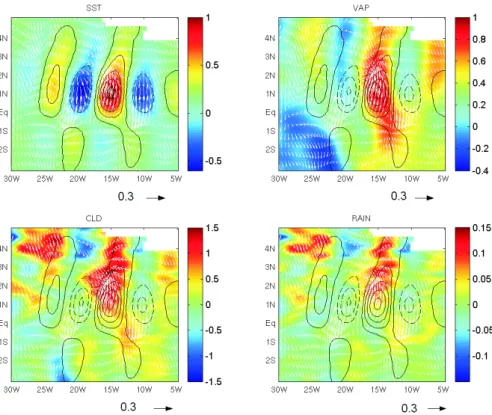
Fig. 8. Regression maps for SST, VAP (mm◦C−1), CLD (10−2mm◦C−1) and RAIN (mm hr−1 ◦C−1). SST contours are plotted in all graphs. Vectors are for wind velocity. Black arrow shows wind velocity approximate to 0.3 ms−1 ◦C−1.
propagating signal in the wind fields, but with the expected larger variability than on the SST fields because of the more rapid changes observed in wind. Nevertheless, the TIWs sig-nals are enhanced by filtering out the lower frequency com-ponent of the wind fields, when applying the same filter as in Fig. 4. Even not being the main focus on this analysis, it is interesting to notice that the wind field displays west-ward propagating disturbances located east of the position where TIWs imprints are expected to be, comparing with the position of the SST instabilities. This result suggests that the wind fields are displaying another kind of atmospheric disturbances, most probably African Easterly Waves (AEW) (Diedhiou et al., 1999). The signal captured in the filtering analysis might contain part of this oscillation. The AEW are westward atmospheric disturbances originated on both north and south of the African Easterly Jet (AEJ), with dominant periodicity of 3 to 9 days (Diedhiou et al., 1999) and lower periodicity of 25–60 days (Janicot and Sultan, 2001).
Unfortunately, this analysis is limited by the QuikSCAT data used in this study, spanning from the second half of 1999 until the end of 2001, leaving only two complete years of data. Spatially, there is a slight difference in the regions where the components are affected. The centre of maximum variability is displaced further north, at around 3◦N, for the zonal component. For the meridional component, although it is possible to observe the influence of the TIWs up to 4◦N,
it is noticeable the larger impact around the equator and 1◦N when compared to the zonal component. Temporally, these figures highlight the features observed in Fig. 4, where in 2001, it is possible to observe strong signals reaching regions located at 4◦N.
3.3 Co-variability of oceanic TIWs and atmospheric fields As shown in the previous section, TIWs signals can be ob-served in wind fields as well as in the SST. Two distinct hy-pothetical mechanisms of this coupled variability were pro-posed by Lindzen and Nigam (1987) and by Wallace et al. (1989), using data from the tropical Pacific. In this sec-tion, these two hypotheses are discussed and evaluated for the tropical Atlantic, using spacebased data from TMI and QuickSCAT. Although we acknowledge the mechanism sug-gested by Small et al. (2003), it is difficult to evaluate the relative importance of the pressure gradient with the datasets used in this study. We suggest that a specific coupled mod-elling study for the tropical Atlantic has to be performed in order to evaluate this mechanism.
Figure 8 shows the regression maps for all the variables, for the entire period available. SST, VAP, CLD and RAIN data used were available from 1998 to 2001. Wind com-ponents were available for 2000 and 2001. As expected, the SST anomalies are confined between the equator and 2◦N. Wind velocities are highly correlated with SST. In
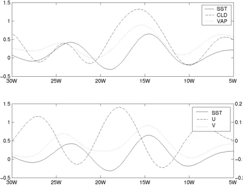
Fig. 9. Longitudinal variations at 1◦N of the filtered anomalies of SST (◦C), cloud liquid water (CLD) (10−2mm), integrated water vapour (VAP) (mm), zonal (U) (ms−1) and meridional (V) (ms−1) wind.
the tropical Atlantic, the meridional component dominates the wind field, so its reaction to the SST anomalies follows the acceleration southwards (northwards) over cold (warm) water. VAP regression seems to be in phase with SST and meridional wind. These results are consistent with the hy-pothesis described by Wallace et al. (1989), that the increased buoyancy-induced mixing reduces wind shear in the bound-ary layer over the warm water. On the other hand, over cold water an opposite situation is expected, where a de-creasing on the buoyancy-induced mixing produces a larger wind shear. The longitudinal variations presented in Fig. 9 essentially reinforce those findings. From Fig. 8, it is notice-able that wind moves across isotherms of SST, accelerating and decelerating, causing convergence and divergence. Wind convergence feeds moisture up into the atmosphere, and the increase of water vapour may be caused by both the surface warming and wind advection.
In addition, CLD and RAIN regressions, which follow very similar spatial patterns, appear to be roughly in phase with wind divergence in the central tropical Atlantic. Fur-ther north, CLD anomalies are accompanied by precipitation changes in the ITCZ whose southern boundary is located at around 4◦N. This more southern position of the Atlantic ITCZ, compared with its Pacific counterpart, makes it more liable to TIWs variability. These results may be an indication that TIWs variability has a high impact in the deep convec-tion associated with the ITCZ. If so, one can expect the year-to-year variability of SST and wind associated with TIWs will reflect on the CLD and RAIN signals.
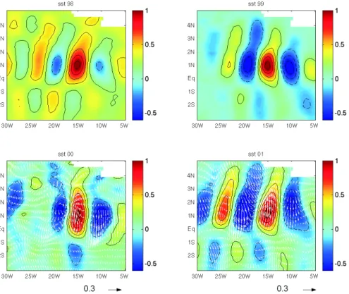
The separate regression maps of SST for each of the years 1998 to 2001 are presented in Fig. 10. Wind vectors appear only in the graphs for 2000 and 2001 because of wind data availability. TIWs signals are present every year, with dif-ferences due to distinct oceanographic conditions. 1998 is a typical example of when the waves can be observed even during anomalous warm conditions. In contrast, during 2000, the equatorial cold tongue was well developed but failed to enhance the signals further west. The wind fields also did not respond in order to adjust to these anomalous conditions. The most active year appears to be 2001, when the influence of TIWs can be observed further north, at around 4◦N, and still, with strong regressions at 25◦W. Wind velocity regres-sions are strong close to the equator, and remain so north of 4◦N.
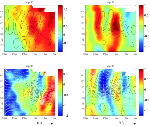
Figures 11, 13, 14 exhibit regression maps for VAP, CLD and RAIN, respectively. Figure 12 shows the mean spatial distribution of RAIN and CLD for the years 2000 and 2001, which might be useful to quantify the impact of TIWs on these fields. 1998 shows the typical pattern of an anoma-lously warm year, with high levels of VAP. Surprisingly, CLD and RAIN spatial distributions follow roughly the av-erage pattern, with maxima at around 2◦N and 4◦N. 2000, which had a well developed cold tongue, does not show the expected imprint of TIWs influence onto the atmospheric fields. Although the equatorial upwelling was strong, the whole tropical Atlantic basin was anomalously cold. This sit-uation inhibited a strong gradient of temperature and, there-fore, the development of the front instabilities. However, this
Fig. 10. Regression maps for SST (colour and contours) for years 1998 to 2001. Vectors are for wind velocity. Black arrow shows wind
velocity approximate to 0.3 ms−1 ◦C−1.
does not indicate that TIWs did not occur. 1999 showed a clear signal of the instabilities, although they were short-lived and, because of this, its influence in the western side of the basin is not well established. CLD and RAIN ex-hibit a more “local” influence, in particular the centre of deep convection at around 4◦N. This centre seems to have been displaced from its mean longitudinal position at 25◦W to around 20◦W.
The most active year of TIWs was 2001 (Fig. 4) and its influence in the atmospheric fields is noticeable in Figs. 11, 13, 14. VAP map regressions show clearly the influence of the wind divergence associated with the waves, although the magnitude of VAP is low, due to the strong upwelling and cold waters associated with it. As the instabilities’ influence in this particular year reaches further north than any other year in this analysis, the observed displacement of CLD and RAIN is north of their usual position. It suggests that the more active the TIWs are, in time and space, the further their influence can be observed.
The results above show the year-to-year impact of the TIWs on the spatial position of the correlated atmospheric fields. Besides, it is important to notice that the regression coefficients maps showed in Figs. 11, 13, 14 can vary as much as 50% if compared with the ”long term” regression coefficients showed in Fig. 8. In order to fully assess the ex-istent coupling between the TIWs and the atmosphere,
spe-cific modelling is needed. Nevertheless, the results presented here support the hypothesis that TIWs variability has a high impact in the deep convection associated with ITCZ in the tropical Atlantic, in particular due to its more southern posi-tion. The year-to-year variability of SST and wind associated with TIWs are clearly reflected in the atmospheric signals.
4 Discussions
The tropical instability waves, although observed for some time in the tropical Atlantic, have never had their SST sig-nature characteristics analysed over the whole basin, as well as their variability from year to year. This work, by using observational satellite data, provides an important study of these instabilities.
The results show that the TIWs clearly vary their position and time of activity, depending on the degree of development of the equatorial cold tongue. The most active year anal-ysed in this study was 2001, when the spectral characteristics could be observed as far as 4◦N. The spectral characteristics of TIWs in the Atlantic obtained by this study and presented in Table 1 are corroborated by previous observations. How-ever, most of those observational studies are based on data from single locations, usually on the equator, and are derived from shorter records. Still, they yield information about the spatial extent of the TIWs. Weisberg and Weingartner (1988)
Fig. 11. Regression maps for VAP (mm◦C−1) for years 1998 to 2001. Contours are for SST from Fig 10. Vectors are for wind velocity. Black arrow shows wind velocity approximate to 0.3 ms−1◦C−1.
found that TIWs have a central periodicity of 25 days, on the equator at 28◦W, with phase speed between 10–50 cm s−1 and wavelengths of around 10◦. Steger and Carton (1991) also showed similar results. Compared with the tropical Pa-cific, these characteristics are slightly different . Pezzi (2003) showed that TIWs at 1◦N in the Pacific during 1999
pre-sented a phase speed of 55 cm s−1, wavelength of 11◦ and
period of 30 days, similar to the results found by Hashizume et al. (2001). These slight differences between the two equa-torial oceans are suggested to be due to the different shape of the oceans, with a higher influence of the continents in the Atlantic case.
Previous theoretical studies, Philander (1978) for the trop-ical Atlantic and Cox (1980) for the troptrop-ical Pacific, showed that the westward propagating instabilities, generated by the shear between the North Equatorial Countercurrent (NECC) and the northern branch of the South Equatorial Current (nSEC), have a period of around 1 month and wavelength of 10◦. More recently, Jochum et al. (2004) showed that
the wavelength of the TIWs can vary from 700 to 1100 km, with a phase speed variation of 30 to 50 cm s−1. The phys-ical reason to expect a certain range in the wave properties is that these instabilities can be generated by simultaneous barotropic and baroclinic instabilities processes. The TIWs energetic characteristics have been studied in more details by Masina et al. (1999) and they have shown that both sources
are important on the TIWs generation and maintenance. Also in a numerical study, Pezzi and Richards (2003) have rein-forced these findings and suggested that TIWs activity varies as function of the level and orientation of the lateral mixing applied on the simulation. Examining the main energy con-version terms of the mean state to eddy energy reveals that both the barotropic and baroclinic energy conversion terms are important for the production of TIWs. The relative role of each of these conversion terms changes as the lateral mix-ing is decreased. As the mixmix-ing coefficient is decreased the TIWs become more energetic and their behavior more irreg-ular, with reduced seasonality while a large diffusivity tends to damp the wave activity producing more organized prop-agation patterns with a stronger seasonality. Therefore it is possible for the TIWs properties to have a range of values.
Moreover, the characteristics of TIWs due to the ther-mal gradient north of the equator, as investigated in this work, have not been shown for the whole tropical Atlantic. These results show that the baroclinic instabilities associated with the thermal gradient have the same characteristics of the barotropic ones, generated by the shear of the surface currents, highlighting that they also contribute to the vari-ability of the TIWs. Our analysis of the SST data derived from satellite slightly differ from one of the Jochum et al. (2004) findings. The authors, from analysis of SST records of the PIRATA array, showed that the TIWs does not have
Fig. 12. Top: Mean spatial distribution of precipitation rates (RAIN) (in mm hr−1) for 2000 and 2001. Bottom: Mean spatial distribution of liquid cloud water (CLD) (in mm) for 2000 and 2001.
a temperature signal at the equator. We would prefer to de-scribe the temperature signals as rather weak at the equator, in particular when compared with their signals further north. However, the differences in interpretation are probably due to the different measurement methods. With satellite retrievals, we use gridded data, which are interpolated, besides its syn-optic view. The moorings are punctual, measuring only at that location.
The imprints of the TIWs are well marked in the wind fields, showing that clearly there are coupled mechanisms as-sociated with the TIWs. Moreover, this study could clearly show that the hypothesis of this coupling as originally sug-gested by Wallace et al. (1989) for the tropical Pacific, is also applied for the tropical Atlantic basin. Although Hashizume et al. (2001) have suggested that Wallace’s hypothesis could be applied for the tropical Atlantic, this had not been shown until now.
Fig. 13. Regression maps for CLD (10−2mm◦C−1) for years 1998 to 2001. Contours are for SST from Fig 10. Vectors are for wind velocity. Black arrow shows wind velocity approximate to 0.3 ms−1 ◦C−1.
As the characteristics of the TIWs have been observed to vary at different latitudes from year to year, it has been pos-sible to test their influence on the ITCZ, which should be larger than its counterpart in the Pacific. As the TMI sen-sor provides simultaneous measurements of several variables that can be associated with the variability of the ITCZ, as integrated water vapour, rain and cloud liquid water, it was possible to analyse this suggested influence. In conjunction with the QuikSCAT wind data the results showed that these atmospheric fields are highly correlated with the SST fields at the timescale associated with the TIWs, which variabil-ity has a high impact in the deep convection associated with ITCZ, in particular due to its more southern position.
5 Conclusions
This work has focused on the SST signature of the TIWs, and characterised their multi-year variability in the Atlantic Ocean, using high-resolution microwave satellite data. The dataset, which has few gaps on a 3-day mean composite, has been filtered with a westward-only 2-D FIR filter. This scheme highlights very well the TIWs by filtering out fea-tures with different spectral characteristics. This analysis showed that TIWs were very active during 2001, and strong signals could be observed far reaching 4◦N.
As wind and SST fields are strongly coupled in the tropics, their interactions allow us to observe the imprints of TIWs in the wind components fields, with similar structures as ob-served in SST. Because the tropical Atlantic basin is influ-enced by the surrounding continents, and due to the closer location of the ITCZ to the equator, compared to its Pacific counterpart, it was possible to identify the impact that these instability waves may have on the ITCZ. Using concurrent multi-year satellite observations of SST, wind, atmospheric water vapour, liquid cloud water and precipitation rates, it was possible to notice variations in water vapour, clouds and rain at the ITCZ, due to the influence of the TIWs. These re-sults suggest that the coupling mechanism of SST and wind through the stability change in the atmospheric boundary layer, as illustrated by Hayes et al. (1989) and Wallace et al. (1989), is supported here.
Acknowledgements. This work was supported by the Conselho
Nacional de Desenvolvimentto Cient´ifico e Tecnol´ogico (CNPq), Brazil, through grant no. 201076/97-7. We acknowledge Remote Sensing Systems (http://www.ssmi.com/) for providing TMI and QuikScat datasets. The authors also are grateful to D. Cromwell for useful comments.
Fig. 14. Regression maps for RAIN (mm hr−1 ◦C−1) for years 1998 to 2001. Contours are for SST from Fig 10. Vectors are for wind velocity. Black arrow shows wind velocity approximate to 0.3 ms−1 ◦C−1.
References
Allen, M. R., Lawrence, S. P., Murray, M. J., Mutlow, C. T., Stock-dale, T. N., Llewellynjones, D. T., and Anderson, D. L. T.: Con-trol of Tropical Instability Waves in the Pacific, Geophys. Res. Lett., 22, 2581–2584, 1995.
Chelton, D. B., Wentz, F. J., Gentemann, C. L., de Szoeke, R. A., and Schlax, M. G.: Satellite microwave SST observations of transequatorial tropical instability waves, Geophys. Res. Lett., 27, 1239–1242, 2000.
Chelton, D. B., Esbensen, S. K., Schlax, G., Thum, N., Freilich, M. H., Wentz, F. J., Gentemann, C. L., McPhaden, M. J., and Schopf, P. S.: Observations of coupling between surface wind stress and sea surface temperature in the eastern tropical Pacific, J. Clim., 14, 1479–1498, 2001.
Cipollini, P., Cromwell, D., Challenor, P. G., and Raffaglio, S.: Rossby waves detected in global ocean colour data, Geophys. Res. Lett., 28, 323–326, 2001.
Contreras, R.: Long-term observations of tropical instability waves, J. Phys. Oceanogr., 132, 2715–2722, 2002.
Cox, M.: Generation and propagation of 30-day waves in a numer-ical model of the Pacific, J. Phys. Oceanogr., 10, 1168–1186, 1980.
Deans, S.: The Radon transform and some of its applications, John Willer, 1983.
Deser, C., Bates, J. J., and Wahl, S.: The Influence of Sea-Surface Temperature-Gradients on Stratiform Cloudiness Along the Equatorial Front in the Pacific-Ocean, J. Clim., 6, 1172– 1180, 1993.
Diedhiou, A., Janicot, S., Viltard, A., de Felice, P., and Laurent, H.: Easterly wave regimes and associated convection over West Africa and tropical Atlantic: results from the NCEP/NCAR and ECMWF reanalysis, Clim. Dyn., 15, 795–822, 1999.
Duing, W., Hisard, P., Katz, E. J., Knauss, J., Meincke, J., Miller, L., Moroshkin, K., Philander, S. G. H., Rybnikov, A., Voigt, K., and Weisberg, R. H.: Meanders and long waves in the equatorial Atlantic, Nature, 257, 280–284, 1975.
Flament, P. J., Kennan, S. C., Knox, R. A., Niiler, P. P., and Bern-stein, R. L.: The three-dimensional structure of an upper ocean vortex in the tropical Pacific Ocean, Nature, 383, 610–613, 1996. Gentemann, C. L., Wentz, F. J., Mears, C. A., and Smith, D. K.: In situ validation of Tropical Rainfall Measuring Mission mi-crowave sea surface temperatures, J. Geophys. Res.-Oceans, 109, art. no. C04 021, 2004.
Halpern, D., Knox, R. A., and Luther, D. S.: Observations of 20-Day Period Meridional Current Oscillations in the Upper Ocean Along the Pacific Equator, J. Phys. Oceanogr., 18, 1514–1534, 1988.
Hansen, D. V. and Paul, C. A.: Genesis and Effects of Long Waves in the Equatorial Pacific, J. Geophys. Res.-Oceans, 89, 431–440, 1984.
Hashizume, H., Xie, S. P., Liu, W. T., and Takeuchi, K.: Local and remote atmospheric response to tropical instability waves: A global view from space, J. Geophys. Res.-Atmos., 106, 10 173– 10 185, 2001.
Hashizume, H., Xie, S. P., Fujiwara, M., Shiotani, M., Watanabe, T., Tanimoto, Y., Liu, W. T., and Takeuchi, K.: Direct observations of atmospheric boundary layer response to SST variations asso-ciated with tropical instability waves over the eastern equatorial Pacific, J. Clim., 15, 3379–3393, 2002.
Hayes, S. P., McPhaden, M. J., and Wallace, J. M.: The Influence of Sea-Surface Temperature on Surface Wind in the Eastern Equa-torial Pacific – Weekly to Monthly Variability, J. Clim., 2, 1500– 1506, 1989.
Hill, K. L., Robinson, I. S., and Cipollini, P.: Propagation charac-teristics of extratropical planetary waves observed in the ATSR global sea surface temperature record, J. Geophys. Res.-Oceans, 105, 21 927–21 945, 2000.
Janicot, S. and Sultan, B.: Intra-seasonal modulation of convection in the West African monsoon, Geophys. Res. Lett., 28, 523–526, 2001.
Jochum, M., Malanotte-Rizzoli, P., and Busalacchi, A. J.: Tropi-cal instability waves in the Atlantic Ocean, Ocean Modelling, 7, 145–163, 2004.
Kennan, S. C. and Flament, P. J.: Observations of a tropical insta-bility vortex, J. Phys. Oceanogr., 30, 2277–2301, 2000. Kummerow, C., Barnes, W., Kozu, T., Shiue, J., and Simpson, J.:
The Tropical Rainfall Measuring Mission (TRMM) sensor pack-age, J. Atmos. Oceanic Technol., 15, 809–817, 1998.
Legeckis, R.: Long waves in the eastern equatorial Pacific Ocean: a view from a geostationary satellite, Science, 197, 1179–1181, 1977.
Lindzen, R. S. and Nigam, S.: On the Role of Sea-Surface Temperature-Gradients in Forcing Low-Level Winds and Con-vergence in the Tropics, J. Atmos. Sci., 44, 2418–2436, 1987. Liu, W. T., Xie, X. S., Polito, P. S., Xie, S. P., and Hashizume,
H.: Atmospheric manifestation of tropical instability wave ob-served by QuikSCAT and tropical rain measuring mission, Geo-phys. Res. Lett., 27, 2545–2548, 2000.
Lumpkin, R. and Garzoli, S. L.: Near-surface circulation in the trop-ical Atlantic Ocean, Deep-Sea Res. Part I, 52, 495–518, 2005. Masina, S. and Philander, S. G. H.: An analysis of tropical
instabil-ity waves in a numerical model of the Pacific Ocean – 1. Spatial variability of the waves, J. Geophys. Res.-Oceans, 104, 29 613– 29 635, 1999.
Masina, S., Philander, S. G. H., and Bush, A. B. G.: An analysis of tropical instability waves in a numerical model of the Pacific Ocean – 2. Generation and energetics of the waves, J. Geophys. Res.-Oceans, 104, 29 637–29 661, 1999.
Menkes, C. E., Kennan, S. C., Flament, P., Dandonneau, Y., Mas-son, S., Biessy, B., Marchal, E., Eldin, G., Grelet, J., Montel, Y., Morliere, A., Lebourges-Dhaussy, A., Moulin, C., Champalbert, G., and Herbland, A.: A whirling ecosystem in the equatorial Atlantic, Geophys. Res. Lett., 29, art. no. 1553, 2002.
Neelin, J. D., Battisti, D. S., Hirst, A. C., Jin, F. F., Wakata, Y., Yamagata, T., and Zebiak, S. E.: ENSO theory, J. Geophys. Res.-Oceans, 103, 14 261–14 290, 1998.
Pezzi, L. P.: Equatorial Pacific Dynamics: Lateral Mixing and Trop-ical Instability Waves, Ph.d. thesis, University of Southampton, 2003.
Pezzi, L. P. and Richards, K. J.: The effects of lateral mixing on the mean state and eddy activity of an equatorial ocean, J. Geophys. Res., 108, doi:10.1029/2003JC001 834, 2003.
Pezzi, L. P., Vialard, J., Richards, K. J., Menkes, C., and Anderson, D. L. T.: Infuence of ocean-atmosphere coupling on the proper-ties of Tropical Instability Waves, Geophys. Res. Lett., 31, 2004. Philander, S. G. H.: Instabilities of zonal equatorial currents, 2, J.
Geophys. Res.-Oceans, 83, 3679–3682, 1978.
Philander, S. G. H. and Pacanowski, R. C.: A model of the sea-sonal cycle in the tropical Atlantic Ocean, J. Geophys. Res., 91, 14 192–14 206, 1986.
Philander, S. G. H., Hurlin, W. J., and Pacanowski, R. C.: Properties of Long Equatorial Waves in Models of the Seasonal Cycle in the Tropical Atlantic and Pacific Oceans, J. Geophys. Res.-Oceans, 91, 14 207–14 211, 1986.
Polito, P. S. and Cornillon, P.: Long baroclinic Rossby waves de-tected by TOPEX/POSEIDON, J. Geophys. Res.-Oceans, 102, 3215–3235, 1997.
Qiao, L. and Weisberg, R. H.: Tropical Instability Wave Kinematics - Observations from the Tropical Instability Wave Experiment, J. Geophys. Res.-Oceans, 100, 8677–8693, 1995.
Small, R., Xie, S.-P., and Wang, Y.: Numerical simulation of atmo-spheric response to Pacific tropical instability waves, J. Clim., 16, 3723–3741, 2003.
Steger, J. M. and Carton, J. A.: Long Waves and Eddies in the Trop-ical Atlantic-Ocean – 1984–1990, J. Geophys. Res.-Oceans, 96, 15 161–15 171, 1991.
Thum, N., Esbensen, S. K., Chelton, D. B., and McPhaden, M. J.: Air-sea heat exchange along the northern sea surface tempera-ture front in the eastern tropical Pacific, J. Clim., 15, 3361–3378, 2002.
Wallace, J. M., Mitchell, T. P., and Deser, C.: The Influence of Sea-Surface Temperature on Sea-Surface Wind in the Eastern Equatorial Pacific – Seasonal and Interannual Variability, J. Clim., 2, 1492– 1499, 1989.
Wang, C. and Weisberg, R.: Ocean circulation influences on sea surface temperature in the equatorial central Pacific, J. Geophys. Res., 106, 19 515–19 526, 2001.
Wang, W. M. and McPhaden, M. J.: The surface-layer heat balance in the equatorial Pacific Ocean. Part I: Mean seasonal cycle, J. Phys. Oceanogr., 29, 1812–1831, 1999.
Weisberg, R. H.: Instability Waves Observed on the Equator in the Atlantic-Ocean During 1983, Geophys. Res. Lett., 11, 753–756, 1984.
Weisberg, R. H. and Weingartner, T. J.: Instability Waves in the Equatorial Atlantic-Ocean, J. Phys. Oceanogr., 18, 1641–1657, 1988.
Xie, S. P., Ishiwatari, M., Hashizume, H., and Takeuchi, K.: Cou-pled ocean-atmospheric waves on the equatorial front, Geophys. Res. Lett., 25, 3863–3866, 1998.