Journal of Geophysical Research: Space Physics
Milne-Eddington inversion for unresolved magnetic structures
in the quiet Sun photosphere
Véronique Bommier1
1LESIA, Observatoire de Paris, PSL Research University, CNRS, Sorbonne Universités, UPMC, University Paris Diderot, Paris, France
Abstract
This paper is first devoted to present our method for modeling unresolved magnetic structures in the Milne-Eddington inversion of spectropolarimetric data. The related definitions and other approaches and different used inversion algorithms are recalled for comparison. In a second part, we apply our method to quiet Sun data outside active regions. We obtain the quiet Sun photospheric magnetic field as composed of unresolved opening and connected magnetic flux tubes, which form a loop carpet of field lines. We then analyze the spatial correlation, which we also observed for the magnetic field vector, in terms of flux tube diameter, distance, and field strength. We find that different observations with the Zurich imaging polarimeter and THEMIS polarimeter mounted on the THEMIS telescope give very close results, and we add results also very close derived from HINODE/Solar Optical Telescope/spectropolarimeter observations analyzed with the same method. We obtain a mean flux tube diameter of 30 km, a mean flux tube distance of 230 km, and a mean flux tube magnetic field of 1.3 kG.1. Introduction
The existence of unresolved structure of the solar magnetic field is obviously to be expected. First insight in this veiled domain was done in a pioneering and visionary work by Stenflo [1973], who revealed the exis-tence of scattered sharp magnetic flux tubes by comparing polarization observations in two lines formed at the same depth in the atmosphere, but of different magnetic sensitivity. From the observation interpretation, he concludes that the solar network is permeated by flux tubes of about 2 kG and diameter 100–300 km. This structure was confirmed by further observations that we report in detail in section 4. On the other hand, network bright points were put in the same category as magnetic flux tubes, and first measurements of their diameter was performed at the Pic-du-Midi by Muller and Keil [1983] who obtain 160 km. The distance between two flux tubes is a complementary datum, which was not clearly determined in all these works. In the present work, we propose new determinations of these two quantities, which are flux tube diameter and distance between flux tubes, from inverted spectropolarimetric observations and their spatial correlations. Our obser-vations are not located in the network but in the internetwork instead as the recent work by Stenflo [2011], who derives there a sharper flux tube diameter of 26–50 km.
The results we present here are directly derived or associated to the results presented in Bommier [2011], where the quiet Sun magnetic field appears as an organized structure with not independent field strength and inclination with more vertical stronger fields and more horizontal weaker fields. This suggests that the photospheric internetwork field has the structure of scattered narrow flux tubes composed of vertical field, which weakens in opening—widening with individual field line bending—with height. In other words, the quiet Sun magnetic field lines form a loop carpet as also proposed from observations by Martínez González
et al. [2007, 2010].
In Bommier [2011] we also reported spatial correlation results for the magnetic field inclination and azimuth. We realized that the magnetic flux tube typical diameter can be easily derived from the correlation length and from the magnetic filling factor, which was also derived in Bommier [2011] following the method described in
Bommier et al. [2009] based on the weak field laws, independently of the UNNOFIT inversion applied to
deter-mine the magnetic field. Bommier et al. [2009] present quiet Sun observations made with the Zurich imaging polarimeter (ZIMPOL) polarimeter mounted on the THEMIS telescope, whereas Bommier [2011] concerns quiet Sun observations made with the THEMIS polarimeter. The two observations differ about the pixel
RESEARCH ARTICLE
10.1002/2016JA022368
Special Section:
Measurement Techniques in Solar and Space Physics: PhotonsKey Points:
• A method is presented to infer unresolved magnetic structure from spectropolarimetric measurements • We obtain a mean internetwork
flux tube diameter 30 km, distance 230 km, and magnetic field 1.3 kG • The solar internetwork magnetic
field would be a carpet of loops connecting the vertical flux tubes
Correspondence to:
V. Bommier, [email protected]
Citation:
Bommier, V. (2016), Milne-Eddington inversion for unresolved magnetic structures in the quiet Sun photo-sphere, J. Geophys. Res. Space Physics,
121, doi:10.1002/2016JA022368.
Received 11 JAN 2016 Accepted 20 MAY 2016
Accepted article online 30 MAY 2016
©2016. American Geophysical Union. All Rights Reserved.
size by a factor of 2 and also about the integration time. The observed regions were also different. We determine the typical flux tube diameter in both cases and find them in very close agreement. A recent deter-mination of the flux tube diameter can be found in Stenflo [2011], from HINODE/Solar Optical Telescope/ spectropolarimeter(SOT/SP) data analyzed with a different method. In order to compare our method with this one, we treated the same HINODE/SOT/SP data with the method and codes of Bommier et al. [2009] and
Bommier [2011]. In order to improve the quality of the results, we have applied pixel selection following Borrero and Kobel [2011, 2012] by analyzing only those pixels where the linear polarization spectral maximum
is larger than 4.5 times the polarimetric noise level. In the present paper we retreat the THEMIS data also with the pixel selection, but the previous results are not strongly modified. The found results for the magnetic filling factor and spatial correlation for the inclination and azimuth, which we present, confirm the results previously obtained for the THEMIS observations. We derive the flux tube diameter for the THEMIS and HINODE obser-vations, which we find in agreement with the flux tube diameter of Stenflo [2011] and in agreement between themselves. This is the object of section 3. It has to be noticed that the typical flux tube diameter we derive is not the result of the observation of one or several flux tubes with individual results. It is instead an order of magnitude derived from large samples of pixels analyzed with statistical methods.
This paper is the occasion to return to the description of our Milne-Eddington inversion method at the basis of the UNNOFIT inversion code [Bommier et al., 2007]. In this code, we modeled the unresolved magnetic structures by introducing a magnetic filling factor and a two-component Milne-Eddington atmosphere. The originality of our method lies in the application of the Levenberg-Marquardt algorithm to both the magnetic and nonmagnetic intensity profiles, together with the magnetic filling factor. In section 2, we first describe what is a Milne-Eddington atmosphere, what are the different inversion techniques, and finally, what are the different approaches applied to determine the magnetic filling factor within the Milne-Eddington inversion.
2. Introduction of a Magnetic Filling Factor in the Milne-Eddington Inversion
2.1. The Milne-Eddington InversionThe aim of this work is the retrieval of the astrophysical magnetic field vector by interpretation of spectropo-larimetric data. However, the theory of line formation in the presence of a magnetic field provides the line spectrum polarization given a magnetic field vector, whereas what is needed for the interpretation is just the opposite. That is why an inversion step is required to determine, given an observed polarization profile, what would be the magnetic field vector responsible for it. Eventually, several different magnetic field vectors may be responsible for the same emitted polarization. These are the ambiguities, among which is the so-called fundamental ambiguity, in which two field vectors symmetrical with respect to the line of sight lead to the same emitted polarization. Then, a full magnetic field vector determination must include the ambiguity reso-lution, which is the last but not the least step of the measurement. As for the inversion, this operation requires an adapted algorithm to be performed. Two types of them can be envisaged.
The first type is interpolation in a grid of models, which has to be first computed given a series of magnetic field vectors. Examples of this type of method can be found in Bommier et al. [1981] for interpretation of the Hanle effect observed in solar prominences and Ishikawa et al. [2014] for chromospheric observations of the Hanle effect. A sophisticated algorithm for performing this kind of inversion is based on the principal component analysis of the observed polarized spectrum. An example of such an analysis can be found in López Ariste and
Casini [2002] also for the Hanle effect observed in solar prominences.
The second type of inversion algorithm is the Levenberg-Marquardt algorithm [Press et al., 1989], in which the algorithm is able to tell how the searched for model parameters have to be modified in the model for decreas-ing the gap between the theoretical and observed signal. The algorithm makes use of the partial derivatives of the modeled signal with respect to the searched for parameters. These derivatives may eventually be numerically evaluated. Besides the Levenberg-Marquardt algorithm, other algorithms have been developed, which are aimed to perform a so-called global minimization, in particular, in order to avoid being trapped in eventual local minima. Some global minimization techniques are the so-called genetic optimization method (see an example in Lagg et al. [2004]). Another global optimization algorithm has been used by Asensio Ramos
et al. [2008] to build their Hanle-Zeeman inversion code HAZEL.
The Levenberg-Marquardt algorithm requires the computation of the partial derivatives of the signal with respect to the model parameters. The lower is the parameter number, the easier is the calculation, also if the model dependence of the parameters is analytical. This is the case of the Milne-Eddington atmosphere
Journal of Geophysical Research: Space Physics
10.1002/2016JA022368
model, which will be described below in more detail, and in this case the inversion is usually denoted as Milne-Eddington inversion. However, more sophisticated models have been used, which have a larger num-ber of defining parameters. In this case, the response functions of the observed signals to the parameters have revealed to be fruitful for determining these partial derivatives, as exploited in the SIR (Stokes Inversion based of Response functions) inversion code [Ruiz Cobo and del Toro Iniesta, 1992].Following section 9.8 of Landi Degl’Innocenti and Landolfi [2004], the Milne-Eddington atmosphere model is characterized as follows. The atmosphere is supposed to be plane parallel, semiinfinite, and in local thermo-dynamic equilibrium (the source function in the line and continuum is the Planck function). The magnetic field vector (strength and direction angles), the absorption coefficient (line and continuum), the line-of-sight velocity component, the Doppler and natural width, all are assumed to be depth independent. The only varying parameter is the Planck function, which is assumed to depend linearly on the continuum optical depth measured along the vertical𝜏c
B = B0+ B1𝜏c
= B0(1 +𝛽𝜏c
)
. (1)
The Planck function then depends on the two parameters B0and B1, but if the analyzed polarization profiles
are scaled to the continuum, finally, only one parameter,𝛽 of the above equation, remains to be determined for characterizing the atmosphere. In this atmosphere model, the transfer equation for the polarized radiation can be analytically solved in the presence of a magnetic field. This was done by Unno [1956] for a normal Zeeman triplet line J = 0→ J′ = 1, later on modified by Rachkovsky [1962, 1967] to take into account the
magneto-optical effects. This is the well-known Unno-Rachkovsky analytical solution of the radiative transfer equation for polarization as can be found in Landi Degl’Innocenti and Landolfi [2004, p. 415]. In the so-called Milne-Eddington inversion, the Levenberg-Marquardt algorithm is applied to this solution for the retrieval of the parameters, which are, namely, (1) the line absorption coefficient𝜂0; (2) the line central wavelength𝜆0; (3) the line Doppler width Δ𝜆D; (4) the line natural width, or in practice the a coefficient of the Voigt function
H(a, v); (5) the atmosphere Milne-Eddington parameter 𝛽; and (6–8) the magnetic field vector coordinates B, 𝜃, 𝜒.
2.1.1. The Number of Independent Parameters
Although it would not be prerequisite that the number of searched for parameters exactly balances the number of independent quantities in the analyzed signal, this is probably preferable. The question arises to determine the number of independent parameters delivered by a spectral line observed in the four Stokes parameters. In our opinion, this number is not so large because the line profile is globally determined by four quantities only, which correspond to the four first parameters of the model, which are, namely, (1) the line spectral depth with respect to the continuum (absorption line); (2) the line central wavelength𝜆0; (3) the line
width; and (4) the line far wings, related to the a coefficient of the Voigt function H(a, v). This assumes that there is no Zeeman component splitting visible in the intensity profile. In solar physics, such a visible Zeeman splitting in the intensity profile would occur in sunspot umbrae only, when the Zeeman splitting is sufficiently larger than the Doppler width. In this paper, we rather consider the case of the quiet solar atmosphere and internetwork. One spectral line observed in Stokes I provides these four parameters only as a global descrip-tion of the line shape. As for the Stokes Q, U, V profiles, when the field is not too large (conditions given in the fourth paragraph of section 2.2), they are not completely independent of Stokes I as for their spectral shapes; see, for instance, the weak field laws as described in Landi Degl’Innocenti and Landolfi [2004, pp. 402–403]. As a consequence each Stokes Q, U, V represents only one additional independent parameter each. Finally, one spectral line observed in the four Stokes parameters provides only seven really independent parameters. In practice, we experienced that the Milne-Eddington parameter𝛽 remained undetermined. However, the Milne-Eddington inversion was nevertheless working and validated by tests.
Increasing the number of simultaneously observed spectral lines is a hopeful way to increase the number of independent observed parameters. The different lines may however be not totally independent. For instance, if they are lines of the same multiplet, their absorption coefficients may be interconnected, as well as their Doppler widths and spectral positions. This question has to be more precisely investigated. Promising tests have been done by Del Toro Iniesta et al. [2010] with the Fe I 6301.5 and 6302.5 Å lines. Although these lines belong to the same multiplet, the number of independent retrieved parameters seems to be increased. Recent observations in 12 spectral lines by Balthasar and Demidov [2012] enable the retrieval of a larger number of parameters, which are assigned to the atmosphere model. In this case the inversion was performed by
applying the SIR code [Ruiz Cobo and del Toro Iniesta, 1992] with a larger number of parameters describing the atmosphere model.
2.2. Taking Into Account the Magnetic Filling Factor
The pioneering work by Stenflo [1973] revealed that the network magnetic field is made of unresolved struc-tures formed by strong fields concentrated in flux tubes, which are embedded in a much weaker or even zero field medium. The analysis of two lines of different magnetic sensitivity but formed at the same depth revealed the existence of kilogauss fields. On the other hand, it is well known that the photospheric average field (outside active regions) is much weaker. This leads to the image of the kilogauss scattered unresolved flux tubes. As a first approximation, this unresolved structure can be modeled by introducing a magnetic filling factor𝛼 in the model, which is assumed to be made of two components, which are, namely, (1) a magnetic component with a magnetic field ⃗Bfilling the𝛼 fraction of space and (2) a nonmagnetic component with zero magnetic field filling the complementary fraction 1 −𝛼 of space. In the future, more continuous field distribu-tion should be obviously envisaged for the model. In the following, we will describe how the two-component model can be used in the frame of the Milne-Eddington approximation.
The mixing of the two components in the observed signal is achieved as follows: ⎧ ⎪ ⎪ ⎨ ⎪ ⎪ ⎩ I =𝛼Im+ (1 −𝛼)Inm Q =𝛼Qm U =𝛼Um V =𝛼Vm , (2)
where (I, Q, U, and V) are the four Stokes parameters, and the indexes “m” and “nm” stand for “magnetic” and “nonmagnetic,” respectively. In the Milne-Eddington atmosphere model, Imdepends on the eight parameters
mentioned above
Im(𝜂0, 𝜆0, Δ𝜆D, a, 𝛽, B, 𝜃, 𝜒) , (3) whereas Inmdepends on the five first parameters only
Inm(𝜂0, 𝜆0, Δ𝜆D, a, 𝛽) . (4)
In principle, these five parameters in Inmshould be assumed to be different from their corresponding ones
in Im, because the atmosphere inside the flux tube is different from the atmosphere outside, given the
presence/absence of magnetic pressure. One would then have 5 + 8 = 13 parameters, to which the𝛼 param-eter has to be added. This results in 14 paramparam-eters to be dparam-etermined with the inversion. However, as also mentioned above, one spectral line brings only seven independent parameters. Therefore, the determination of the 14 parameters would require a multiline analysis.
In a first step, we began with single-line analysis, together with the simplifying assumption that the five param-eters of Inmare identical to the five first parameters of Im. The number of parameters to be determined is
then reduced to eight, to which the𝛼 parameter has to be added. This results in nine parameters to be deter-mined from the inversion, which are still too many, so that indeterminancy is to be expected. We investigated the single-line Milne-Eddington inversion in these conditions in Bommier et al. [2007]. For doing this, we pre-pared 183,600 test profiles by applying the Unno-Rachkovsky solution to a series of magnetic field and filling factor values (see the publication for details). Some theoretical noise typical of contemporary observations was added to the test profiles. These test profiles were submitted to the Milne-Eddington inversion in the two-component atmosphere simplified as described above. The parameters retrieved from the inversion can then be compared to the theoretical ones, and the conclusions were as follows.
The number of parameters to be retrieved, nine, is higher than the number of independent parameters avail-able in the polarized profile, seven. An indeterminancy remains, which is that the magnetic field strength
Band the magnetic filling factor𝛼 cannot be individually determined (at least when the Zeeman splitting remains smaller than the Doppler width—when the Zeeman component would be separated in the profile, additional information would be brought, which would enable the individual parameter determination). But their product𝛼B, which can be denoted as the “local average magnetic field strength,” is correctly retrieved by the inversion, as well as the field inclination and azimuth. The test histograms, which confirm this result,
Journal of Geophysical Research: Space Physics
10.1002/2016JA022368
Figure 1. Sunspot of NOAA 11084 observed on 2 July 2010 at 01:00 by SDO/HMI. Inclination of the magnetic field vector
with respect to the line of sight. (bottom) VFISV inversion assuming magnetic filling factor unity (i.e., homogeneous magnetic field). (top) Our UNNOFIT inversion assuming the presence of a nonunity magnetic filling factor.
can be found in Figures 4 and 5 of Bommier et al. [2007] for the Fe I 6302.5 Å line and Figures 6 and 7 for the 6301.5 Å line inversion. These magnetic field vectors are well determined, although the number of retrieved parameters, eight, remains larger than the number of independent parameters available in a single line. The Milne-Eddington parameter𝛽 is not really determined, but this surprisingly does not prevent a determination of the field vector coordinates, as shown by the tests.
The fact that the field inclination and azimuth are correctly determined has an interesting consequence. Figure 1 displays the inclination angles obtained by inverting sunspot data obtained with Solar Dynamics Observatory/Helioseismic and Magnetic Imager (SDO/HMI) in the Fe I 6173 Å line. A cubic spline interpolation was applied to the spectral data that are made of six frequency points only. Two frequency points were added
between each couple of initial frequency points, by using the cubic spline interpolation. The continuum was taken at the highest intensity level of the six frequency points. Concerning the magnetic filling factor, it is usually unity in spot umbrae and penumbrae, whereas it departs the larger from unity the farther from the spot center. Figure 1 (top) displays the result of the two-component Milne-Eddington inversion as described above. Figure 1 (bottom) displays the result of the very fast inversion of the Stokes vector (VFISV) inversion [Borrero et al., 2011], which is also a Milne-Eddington inversion, also able of a nonunity filling factor but using a different approach. However, in Figure 1 the magnetic filling factor was forced to unity in the VFISV inversion. It can be seen that in this case the field inclinations are close to horizontal outside the sunspot, whereas with our UNNOFIT inversion various inclinations are obtained, which were validated by the tests of Bommier
et al. [2007] in the frame of the existence of unresolved flux tubes as revealed by Stenflo [1973]. The visible
difference between the field inclinations retrieved with or without the hypothesis of nonunity magnetic fill-ing factor shows that the two-component inversion, even simplified, is mandatory for a correct field vector determination outside sunspots.
The two-component Milne-Eddington inversion as described above finally does not provide the magnetic filling factor𝛼. In Bommier et al. [2009, equation (6)], we proposed a method for determining 𝛼 in a second step. This method is based on the weak field laws and on the field inclination determination, which is correctly performed by the inversion as mentioned above. This was applied outside active regions in Bommier et al. [2009] and in Bommier [2011]. This is resumed and extended in the next section. The result was kilogauss fields filling 1 or 2% of space, extending the network result of Stenflo [1973] to the quiet Sun.
Another approach was previously developed to solve the indetermination in the two-component Milne-Eddington single-line inversion. This approach was proposed by Skumanich and Lites [1987] and Lites and
Skumanich [1990]. The magnetic filling factor𝛼 is alternatively determined before the inversion. This requires
the prerequisite knowledge of the nonmagnetic profile Inm. The authors propose to achieve this
determi-nation by averaging over the observed solar region. Either the whole region is averaged, or the less active part of it, or the 8 pixels surrounding each pixel in quiet regions as done by Orozco Suárez et al. [2007] on HINODE/SOT/SP data. Once the nonmagnetic intensity profile is determined by averaging,𝛼 is derived by comparing this profile to each pixel intensity profile. Orozco Suárez et al. [2007] derive then hectogauss fields filling a dozen percent of space, which is compatible with our result of kilogauss field filling 1 or 2% of space, given the result mentioned above that the two-component Milne-Eddington inversion determines only the product𝛼B, which is the “local average magnetic field.” As for their 𝛼B, hectogauss fields filling a dozen percent of space are equivalent to kilogauss fields filling 1 or 2% of space. The result about hectogauss fields is not surprising, given the fact that we observed that the intensity profile is rather variable from 1 pixel to another one, which results in an average intensity profile rather different from the profile in each pixel. This results in nonvery small filling factors. It may also be remarked that the magnetic field is anyways present in all pixels, which has an always line broadening effect. Accordingly, averaging over pixels does not suppress the magnetic field effect. Our method, based on weak field laws, is better found to determine𝛼, and our result, which we describe in the next section, is in agreement with Stenflo [1973].
3. Application: Flux Tube Diameter Inferred From Spatial Correlation in the
Observed Surface Magnetic Field
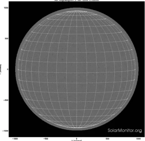
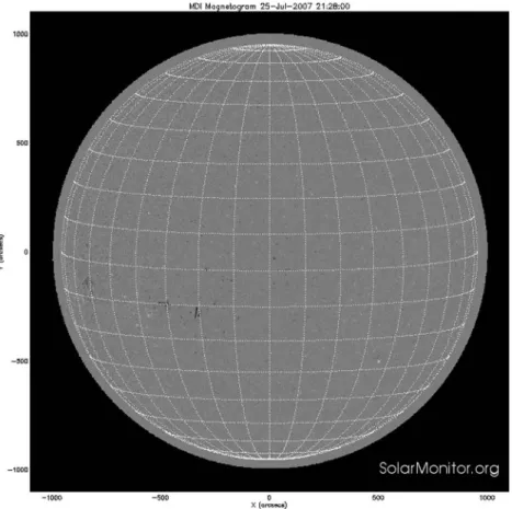
We observed the quiet Sun magnetic field on the 5–6 July 2008 with the ZIMPOL mounted on the THEMIS telescope [Bommier et al., 2009] and on the 25 July 2007 with the THEMIS polarimeter of the same telescope [Bommier, 2011]. These observations were performed at disk center, which was void of any active region. These are spectropolarimetric observations with the spectrograph slit positioned on the disk image. For the ZIMPOL/THEMIS observation, the slit was let fixed on the disk image, and several exposures were performed. In these conditions, it is not possible to plot a 2-D map of the observed magnetic field. The magnetic context of this observation is given in Figure 2. The THEMIS/THEMIS observation was also located at disk center and was composed on repeated small scans of the slit on the solar disk image. The longitudinal magnetic field is represented in Figure 3, where it can be seen that the observed region was essentially internetwork. The magnetic context is given in Figure 4. Both observations were performed during the activity minimum, where the number of active regions is very low.
Journal of Geophysical Research: Space Physics
10.1002/2016JA022368
Figure 2. Context of the THEMIS observation (ZIMPOL) performed at disk center on 5–6 July 2008. Longitudinal
magnetic field.
The spectropolarimetric line profiles were inverted with the UNNOFIT code [Landolfi et al., 1984]. The code accounts for the unresolved structure of the magnetic field via the so-called magnetic filling factor, which was introduced in the UNNOFIT inversion code as described above and in Bommier et al. [2007].
From test profiles, Bommier et al. [2007, Figure 4] show that the inversion is not able to provide𝛼 and B sep-arately, probably due to insufficient incoming independent parameters. Nevertheless, the product𝛼B, which is the local average magnetic field, is correctly retrieved by the inversion. Even if the result is well known for the longitudinal magnetic field component𝛼B cos 𝜃, we have shown in Bommier et al. [2007, Figure 4] that it applies to the field strength𝛼B. Bommier et al. [2009] and Bommier [2011] then introduce an independent estimation of𝛼 directly from the Stokes profiles by applying the weak field laws as described in equations (1)–(6) of Bommier et al. [2009]. The field line of sight (LOS) inclination obtained by the inversion is used in the weak field law application. From the𝛼B value determined by the UNNOFIT inversion and from the 𝛼 value independently estimated from the Stokes profiles, the magnetic field strength B can be finally derived.
Borrero and Kobel [2011, 2012] have shown that the quality of Milne-Eddington inversions is improved if pixel
selection is applied. Their recommended selection criterion is to retain for analysis only those pixels where
Figure 3. THEMIS observation at disk center in a quiet region on 25 July 2007 in the Fe I 6302.5 Å line. Longitudinal
magnetic field. The color scale ranges from black to white from−92to+92G. The observations were composed of 15 repeated slit scans of ten 0.3 arcsec steps. The slit length was 16 arcsec, and the pixel size along the slit was 0.21 arcsec. This map was corrected from anamorphosis.
Figure 4. Context of the THEMIS observation (THEMIS polarimeter) performed at disk center on 25 July 2007.
Longitudinal magnetic field.
the spectral maximum of the linear polarization degree√Q2+ U2∕I is larger than 4.5 times the polarimetric
noise level. We have reanalyzed both series of data by applying this selection. The new results are visible in Figure 5 for the filling factor histogram (logarithmic scale), 6 for the filling factor as a function of the magnetic field strength (logarithmic coordinates), and 7 for the field strength versus horizontality dependence. The results are not very different from the previous ones where no selection had been applied [Bommier et al., 2009; Bommier, 2011]. The larger is the noise level, the higher is the selection effect. We have different noise levels in our different samples. We determine it by computing the standard deviation of Q∕I, U∕I, V∕I in the line neighboring continuum. By so doing we have determined noise levels of 2 × 10⁻⁴in the ZIMPOL/THEMIS
data [Bommier et al., 2009] and 1.1 × 10⁻³in the THEMIS/THEMIS data [Bommier, 2011].
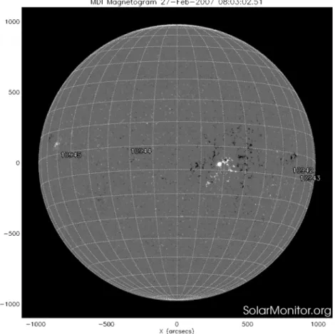
For the ZIMPOL/THEMIS data, it can be seen in Figure 5 that the most probable value of𝛼 in these data is log𝛼 = −2, which corresponds to 𝛼 = 0.01. The linear fit in Figure 6 results in 𝛼 = 13∕B with B in Gauss, so that the typical flux tube magnetic field is B = 1.3 kG in these data. For the THEMIS/THEMIS data, Figure 5 shows that the most probable value of𝛼 in these data is log 𝛼 = −1.7, which corresponds to 𝛼 = 0.02. The linear fit in Figure 6 gives𝛼 = 32∕B with B in Gauss, so that the typical flux tube magnetic field is B = 1.6 kG in these data. We applied the same analysis method to the Fe I 6302.5 Å spectropolarimetric data obtained by HIN-ODE/SOT/SP on 27 February 2007 in a quiet region at disk center. The longitudinal magnetic field map is given in Figure 8. It can be seen that the observed region was essentially internetwork. The magnetic context is given in Figure 9. This observation was also performed during the activity minimum. These data were also analyzed by Stenflo [2010, 2011, 2012] and by Lites et al. [2008]. The magnetic filling factor histogram in Figure 5 shows that the most probable filling factor is log𝛼 = −1.5, which corresponds to 𝛼 = 0.03. The histogram decreases less than does the THEMIS ones on the𝛼 = 1 side. This is probably related to the polarimetric noise level, which is higher in the HINODE than in the THEMIS data. Indeed, we find a polarimetric noise of 1.7 × 10⁻³in
these HINODE data. Once the filling factor is determined by applying the weak field laws complemented by the field LOS inclination determined by the inversion as in Bommier et al. [2009], the magnetic field B can be
Journal of Geophysical Research: Space Physics
10.1002/2016JA022368
Figure 5. Histogram of the magnetic filling factor derived from the weak field laws following the method described in Bommier et al. [2009]. The pixel selection of linear polarization spectral maximum larger than 4.5 times the polarimetric
Figure 6. Magnetic field strength and magnetic filling factor derived following the method described in Bommier et al.
[2009]. A linear fit was applied whose equation is displayed. The pixel selection of linear polarization spectral maximum larger than 4.5 times the polarimetric noise level was performed following Borrero and Kobel [2012].
Journal of Geophysical Research: Space Physics
10.1002/2016JA022368
Figure 7. Magnetic field strength as a function of the horizontality, which is the angle between the field vector and the
horizontal plane. The pixel selection of linear polarization spectral maximum larger than 4.5 times the polarimetric noise level was performed following Borrero and Kobel [2012].
Figure 8. HINODE/SOT/SP observation at disk center in a quiet region on 27 February 2007 in the Fe I 6302.5 Å line.
Longitudinal magnetic field. The color scale ranges from black to white from−1450to+1450G. The scan step was 0.15 arcsec. The scan length was 108 arcsec. The slit length was 164 arcsec, and the pixel size along the slit was 0.16 arcsec.
derived from the inversion result that provides𝛼B. For the HINODE data, the magnetic field and filling factor are found to behave as𝛼 =30∕B as given by the linear fit in Figure 6, so that the magnetic field corresponding to the most probable value𝛼 =0.03 is B=1 kG.
The linear behavior of the scatterplots of Figure 6 results from the fact that𝛼B is rather constant in the quiet Sun. The log-log system of plot coordinates makes the linear behavior more pronounced.
An error evaluation was performed in Bommier et al. [2009]. The relative error Δ𝛼∕𝛼 on the 𝛼 determination is 0.5 for the ZIMPOL/THEMIS data [Bommier et al., 2009, equation (7)], which have the best polarimetric accuracy, and 0.9 for the HINODE data, which have a worse polarimetric accuracy. But the width of the𝛼 histogram is in any case larger than the inaccuracy, which shows that it reflects the variety of possible field strengths, from a few gauss to the kilogauss, that coexist in the solar atmosphere. The selection effect is not very important in the ZIMPOL/THEMIS results where𝛼 is rather well determined, whereas it is more important in the HINODE data where𝛼 is only poorly determined. However, the results of all our samples are found in good agreement. This shows that the selection effect usefully compensates for the noise effect.
In addition, the spatial correlation of the pixel averaged magnetic field vector was studied in all the series of data. The correlation was plotted separately for the inclination and azimuth angles. These plots are visible in Figure 10 of Bommier [2011] for the THEMIS/THEMIS data and Figure 11 of Bommier [2011] for the ZIMPOL/ THEMIS data and in Figure 10 of the present paper for the HINODE data. Below, we discuss the correlation length, which is the half width at half maximum of the spatial autocorrelation function. As we have separately plotted the autocorrelation for the field inclination and azimuth, we have to finally average between the two cases to derive a unique correlation length. For the THEMIS/THEMIS data, the correlation length is 2 pixels for
Journal of Geophysical Research: Space Physics
10.1002/2016JA022368
Figure 9. Context of the HINODE/SOT/SP observation performed at disk center on 27 February 2007. Longitudinal
magnetic field. The grid mesh size is 166 arcsec at disk center, which is similar to the scan size. However, the disk center, which is also the scan center, is 20∘in heliocentric angle apart from the closest active region center, which is large.
the inclination and 1 pixel for the azimuth. Therefore, we consider that the field direction correlation length is the average, which is 1.5 pixel. In these observations the pixel size was 0.21 arcsec, which results in a correlation length𝓁c= 228 km. For the ZIMPOL/THEMIS data, we estimate from the bumps of the curve that the halfwidth is 1 pixel for the inclination and 0.5 pixels for the azimuth, which leads to an average of 0.75 pixels. The ZIMPOL pixel size was 0.53 arcsec. This leads to a correlation length𝓁c= 288 km. For the HINODE data, the half width
is 2 pixels for the inclination. For the azimuth, we find that the average shape of the curve corresponds to a peak half width of 1 pixel, even if the first curve point after the central zero notably deviates from the average. Thus, the average for the HINODE data is 1.5 pixels. The HINODE pixel size is 0.16 arcsec, which results in a correlation length𝓁c= 174 km.
In Figure 7, it is shown that the weakest fields are the most horizontal ones and the strongest fields the most vertical ones, in the two series of THEMIS data and in the the HINODE data. This leads us to describe the photospheric field as opening and connected flux tubes. The question arises as to whether the magnetic𝛼 fraction of a pixel is made all in one piece or consists of several smaller and separate pieces with fractional sum
𝛼. The fact that we observe a spatial correlation suggests the smallest possible number of separate pieces.
Considering then the all in one piece scheme, given a correlation length𝓁cand a magnetic filling factor𝛼, the flux tube diameter becomes𝓁c
√
𝛼, whereas two adjacent flux tubes lie 𝓁capart. A similar expression can be
seen in equation (5) of Stenflo [2011], a paper to which we compare our results in the following subsection. We thus obtain a flux tube diameter 32 km and a flux tube distance 228 km for the THEMIS/THEMIS data, a flux tube diameter 29 km and a flux tube distance 288 km for the ZIMPOL/THEMIS data, and a flux tube diameter 30 km and a flux tube distance 174 km for the HINODE data. The three values of flux tube diameter are in a remarkable agreement. Accordingly, we can claim that from different observations we derive a value of 30 km for the flux tube diameter. For the mean flux tube distance we obtain 230 km. For the mean flux tube
Figure 10. HINODE/SOT/SP observation at disk center in a quiet region on 27 February 2007 in the Fe I 6302.5 Å line.
Autocorrelation along the slit of the inclination and of the azimuth angles, following the method described in
Bommier [2011].
magnetic field we have 1.3 kG for the ZIMPOL/THEMIS data, 1.6 kG for the THEMIS/THEMIS data, and 1 kG for the HINODE data. We finally obtain 1.3 kG as a typical value of the flux tube magnetic field.
4. Comparison With Other Determinations
In a fundamental and pioneering work Stenflo [1973] determines typical flux tube field strength of about 2 kG and diameter of 100–300 km in the network, from polarization ratios of two Fe I lines at 5250 and 5247 Å. This result was later on fully confirmed by Zayer et al. [1989], who obtain flux tube field strength between 1.5 and 2.0 kG and flux tube diameter of 150 km in their cylindrical model, also in network regions and also via this line ratio, which was complemented by another infrared line couple. We find this result fully com-patible with ours because our observations are located in the internetwork instead, where the field may be expected to be sparser with narrower flux tubes of the same field strength as we obtain. Stenflo and Harvey [1985] observed various regions, from the most quiet ones with no visible magnetic flux to strong plages with large Zeeman-effect polarization. However, they similarly conclude that the flux tube properties seem to be rather constant, with field strength about 1 kG, in particular, whereas the magnetic filling factor varies by a factor of 6. In internetwork observations, Wang et al. [1985], who assume field strengths of the kilogauss order, obtain that the real size of the smallest visible elements is about 35–130 km, which is compatible also with our result. Solanki and Stenflo [1984] also observed regions ranging from the quiet Sun to strong plages. On the contrary, they used a large number of lines. They determined a rather constant flux tube field strength rang-ing from 1.2 to 1.7 kG in all these regions, which is also fully compatible with the value we obtain. Muller and
Keil [1983] assimilated flux tubes with network bright points. They determined a size of 0.22 arcsec, which is
160 km, for the bright points diameter observed at the Pic-du-Midi. This result is confirmed by the more recent observations at the Swedish Solar Tower by Berger et al. [2007]. With the Sunrise Filter Imager on board the Sunrise balloon, Riethmüller et al. [2014] determined an observed average bright point diameter of 334 km but obtained a 129 km diameter from a simulation (without degradation for simulating observations). As these
Journal of Geophysical Research: Space Physics
10.1002/2016JA022368
observations are located in the network, whereas ours are in the internetwork, our results seem in full coher-ence for the flux tube field strength, which seems rather constant, as well as for the flux tube diameter, which seems quite smaller in the internetwork than in the network.Stenflo [2011, Figure 11] analyzed the same HINODE/SOT/SP data as us. He derived a most probable flux tube
diameter 26 km or 50 km, which depends on an extrapolation in the data treatment following Stenflo [2010]. Our result of 30 km is in full agreement with both possibilities. It lies in between. As for the flux tube field strength he derives 840 G, which is not so different from the value of 1 kG we derived for the same data. Interestingly, Balthasar and Demidov [2012] obtained similar results about the simultaneous existence of strong (1.5–2.0 kG) and weak (50–150 G) magnetic fields. The strongest fields were observed at a lower alti-tude because they were observed in the center of the disk, whereas the weaker fields were observed closer to the limb, which corresponds to an inclined line of sight with respect to the solar surface, therefore to a higher altitude in the solar atmosphere. Their observations were performed during the solar minimum on 3 February 2009 with the Solar Telescope for Operative Prediction telescope at the Sayan observatory (Russia). The spatial resolution was not so large. Fifteen spectral lines were however simultaneously observed and analyzed. A pixel selection based on the circular polarization level was performed. The spectropolarometric analysis was done by applying the SIR code [Ruiz Cobo and del Toro Iniesta, 1992]. The high number of lines enabled an analysis within a two-component atmosphere model weighted by a magnetic filling factor. The smaller magnetic filling factors (0.005–0.041) are associated to the strongest fields, whereas filling factors larger than 0.5 are found for the weak fields, in excellent agreement with our results. This leads to the same image as ours of vertical but opening kilogauss flux tubes, thus forming a loop carpet made of field lines, as also suggested from observations by Martínez González et al. [2007, 2010].
Recently, Mein et al. [2016], by applying a measurement analysis based on polarization profile moments and Zeeman splitting, showed that unresolved solar magnetic fields seem not to be weaker than kilogauss (see their Figures 14, 17, and 23), in full agreement with our result.
5. Conclusion
In this paper we have reanalyzed ZIMPOL/THEMIS and THEMIS/THEMIS data of Bommier et al. [2009] and
Bommier [2011] by applying them a pixel selection following Borrero and Kobel [2011, 2012] in order to
improve the reliability of the results. We have analyzed with the same methods HINODE/SOT/SP data of the quiet Sun. In all these data we derive the magnetic filling factor independently of the Milne-Eddington inver-sion. The inversion results display a spatial correlation comparable to the pixel size. We assumed that the magnetic𝛼 fraction of a pixel is made all in one piece. From the observed spatial correlation, we derive the mean pixel flux tube and average distance between flux tubes from the magnetic filling factor and correlation length values. We obtain very close flux tube diameter values from our different observations. We obtain the mean value 30 km for the flux tube diameter, 230 km for the average distance between flux tubes, and 1.3 kG for the mean flux tube field strength. This is similar to the minimum flux tube width of 10 km estimated by
Priest [2014] on theoretical grounds.
References
Asensio Ramos, A., J. Trujillo Bueno, and E. Landi Degl’Innocenti (2008), Advanced forward modeling and inversion of Stokes profiles resulting from the joint action of the Hanle and Zeeman effects, Astrophys. J., 683, 542–565, doi:10.1086/589433.
Balthasar, H., and M. L. Demidov (2012), Spectral inversion of multiline full-disk observations of quiet Sun magnetic fields, Solar Phys., 280(2), 355, doi:10.1007/s11207-012-9981-0.
Berger, T. E., L. Rouppe van der Voort, and M. Löfdahl (2007), Contrast analysis of solar faculae and magnetic bright points, Astrophys. J., 661, 1272–1288, doi:10.1086/517502.
Bommier, V. (2011), The quiet Sun magnetic field: Statistical description from THEMIS observations, Astron. Astrophys., 530, A51, doi:10.1051/0004-6361/201015761.
Bommier, V., S. Sahal-Brechot, and J. L. Leroy (1981), Determination of the complete vector magnetic field in solar prominences, using the Hanle effect, Astron. Astrophys., 100, 231–240.
Bommier, V., E. Landi Degl’Innocenti, M. Landolfi, and G. Molodij (2007), UNNOFIT inversion of spectro-polarimetric maps observed with THEMIS, Astron. Astrophys., 464, 323–339, doi:10.1051/0004-6361:20054576.
Bommier, V., M. Martínez González, M. Bianda, H. Frisch, A. Asensio Ramos, B. Gelly, and E. Landi Degl’Innocenti (2009), The quiet Sun magnetic field observed with ZIMPOL on THEMIS. I. The probability density function, Astron. Astrophys., 506, 1415–1428, doi:10.1051/0004-6361/200811373.
Borrero, J. M., and P. Kobel (2011), Inferring the magnetic field vector in the quiet Sun. I. Photon noise and selection criteria,
Astron. Astrophys., 527, A29, doi:10.1051/0004-6361/201015634.
Borrero, J. M., and P. Kobel (2012), Inferring the magnetic field vector in the quiet Sun. II. Interpreting results from the inversion of Stokes profiles, Astron. Astrophys., 547, A89, doi:10.1051/0004-6361/201118238.
Acknowledgments
Based on observations made with the French-Italian telescope THÉMIS operated by the CNRS and CNR on the island of Tenerife in the Spanish Observatorio del Teide of the Instituto de Astrofísica de Canarias. HINODE, Japanese for “Sunrise” and formerly Solar-B, is a solar satellite mission developed, launched, and operated by the Institute of Space and Astro-nautical Science (ISAS)—a division of the Japanese Aerospace Exploration Agency (JAXA)—in collaboration with space agency partners from the National Astronomical Obser-vatory of Japan (NAOJ), the United Kingdom, and the United States. The Solar Dynamics Observatory (SDO) is the first mission launched for NASA’s Living With a Star (LWS) Program. THÉMIS data are available at http://bass2000.bagn.obs-mip.fr/Tarbes/. HINODE/SOT/SP data are available at http://www.csac.hao.ucar.edu/csac/ archive.jsp (thanks to B. Lites). Figures 2, 3, and 9: data supplied courtesy of SolarMonitor.org and of the SOHO/MDI and SOHO/EIT consortia. SOHO is a project of international cooperation between ESA and NASA. For the data inversion, this work was granted access to the HPC resources of MesoPSL financed by the Region Ile de France and the project Equip@Meso (reference ANR-10-EQPX-29-01) of the Investissements d’Avenir program supervised by the Agence Nationale
pour la Recherche. We are grateful to
the THÉMIS team, B. Gelly, A. López Ariste, and C. Le Men, to the ZIMPOL, team and particularly to M. Bianda for their kind assistance during the observations, and to B. Lites for the level-1 HINODE/SOT/SP data. We are grateful to an anonymous referee for a careful reading of our paper.
Borrero, J. M., S. Tomczyk, M. Kubo, H. Socas-Navarro, J. Schou, S. Couvidat, and R. Bogart (2011), VFISV: Very fast inversion of the Stokes vector for the helioseismic and magnetic imager, Solar Phys., 273, 267–293, doi:10.1007/s11207-010-9515-6.
Del Toro Iniesta, J. C., D. Orozco Suárez, and L. R. Bellot Rubio (2010), On spectropolarimetric measurements with visible lines, Astrophys. J.,
711, 312–321, doi:10.1088/0004-637X/711/1/312.
Ishikawa, R., A. Asensio Ramos, L. Belluzzi, R. Manso Sainz, J. Št ˇepán, J. Trujillo Bueno, M. Goto, and S. Tsuneta (2014), On the inversion of the scattering polarization and the hanle effect signals in the Hydrogen Ly𝛼line, Astrophys. J., 787(2), 159, doi:10.1088/0004-637X/787/2/159.
Lagg, A., J. Woch, N. Krupp, and S. K. Solanki (2004), Retrieval of the full magnetic vector with the He I multiplet at 1083 nm. Maps of an emerging flux region, Astron. Astrophys., 414, 1109–1120, doi:10.1051/0004-6361:20031643.
Landi Degl’Innocenti, E., and M. Landolfi (2004), Polarization in Spectral Lines, Astrophysics and Space Science Library, vol. 307, Kluwer Acad., Dordrecht, Netherlands.
Landolfi, M., E. Landi Degl’Innocenti, and P. Arena (1984), On the diagnostic of magnetic fields in sunspots through the interpretation of Stokes parameters profiles, Solar Phys., 93, 269–287, doi:10.1007/BF02270839.
Lites, B. W., and A. Skumanich (1990), Stokes profile analysis and vector magnetic fields. V—The magnetic field structure of large sunspots observed with Stokes II, Astrophys. J., 348, 747–760, doi:10.1086/168284.
Lites, B. W., et al. (2008), The horizontal magnetic flux of the quiet-Sun internetwork as observed with the hinode spectro-polarimeter,
Astrophys. J., 672, 1237–1253, doi:10.1086/522922.
López Ariste, A., and R. Casini (2002), Magnetic fields in prominences: Inversion techniques for spectropolarimetric data of the He I D3line,
Astrophys. J., 575, 529–541, doi:10.1086/341260.
Martínez González, M. J., M. Collados, B. Ruiz Cobo, and S. K. Solanki (2007), Low-lying magnetic loops in the solar internetwork,
Astron. Astrophys., 469, L39—L42, doi:10.1051/0004-6361:20077505.
Martínez González, M. J., R. Manso Sainz, A. Asensio Ramos, and L. R. Bellot Rubio (2010), Small magnetic loops connecting the quiet surface and the hot outer atmosphere of the Sun, Astrophys. J., 714, L94—L97, doi:10.1088/2041-8205/714/1/L94.
Mein, P., H. Uitenbroek, N. Mein, V. Bommier, and M. Faurobert (2016), Fast inversion of Zeeman line profiles using central moments. II. Stokes V moments and determination of vector magnetic fields, A&A, 591, A64, doi:10.1051/0004-6361:201525769.
Muller, R., and S. L. Keil (1983), The characteristic size and brightness of facular points in the quiet photosphere, Solar Phys., 87, 243–250, doi:10.1007/BF00224837.
Orozco Suárez, D., et al. (2007), Strategy for the inversion of hinode spectropolarimetric measurements in the quiet Sun, Publ. Astron. Soc.
Jpn, 59, S837–S844, doi:10.1093/pasj/59.sp3.S837.
Press, W. H., B. P. Flannery, S. A. Teukolsky, and W. T. Vetterling (1989), Numerical Recipes, Cambridge Univ. Press, Cambridge, U. K. Priest, E. (2014), Magnetohydrodynamics of the Sun, Cambridge Univ. Press, Cambridge, U. K.
Rachkovsky, D. N. (1962), Izvestiya Ordena Trudovogo Krasnogo Znameni Krymskoj Astrofizicheskoj Observatorii, 148, vol. 27. Rachkovsky, D. N. (1967), Izvestiya Ordena Trudovogo Krasnogo Znameni Krymskoj Astrofizicheskoj Observatorii, 56, vol. 37. Riethmüller, T. L., S. K. Solanki, S. V. Berdyugina, M. Schüssler, V. Martínez Pillet, A. Feller, A. Gandorfer, and J. Hirzberger (2014),
Comparison of solar photospheric bright points between Sunrise observations and MHD simulations, Astron. Astrophys., 568, A13, doi:10.1051/0004-6361/201423892.
Ruiz Cobo, B., and J. C. del Toro Iniesta (1992), Inversion of stokes profiles, Astrophys. J., 398, 375–385, doi:10.1086/171862. Skumanich, A., and B. W. Lites (1987), Stokes profile analysis and vector magnetic fields. I—Inversion of photospheric lines,
Astrophys. J., 322, 473–482, doi:10.1086/165743.
Solanki, S. K., and J. O. Stenflo (1984), Properties of solar magnetic fluxtubes as revealed by Fe I lines, Astron. Astrophys., 140, 185–198. Stenflo, J. O. (1973), Magnetic-field structure of the photospheric network, Solar Phys., 32, 41–63, doi:10.1007/BF00152728. Stenflo, J. O. (2010), Distribution functions for magnetic fields on the quiet Sun, Astron. Astrophys., 517, A37,
doi:10.1051/0004-6361/200913972.
Stenflo, J. O. (2011), Collapsed, uncollapsed, and hidden magnetic flux on the quiet Sun, Astron. Astrophys., 529, A42, doi:10.1051/0004-6361/201016275.
Stenflo, J. O. (2012), Scaling laws for magnetic fields on the quiet Sun, Astron. Astrophys., 541, A17, doi:10.1051/0004-6361/201218939. Stenflo, J. O., and J. W. Harvey (1985), Dependence of the properties of magnetic fluxtubes on area factor or amount of flux, Solar Phys., 95,
99–118, doi:10.1007/BF00162640.
Unno, W. (1956), Line formation of a normal Zeeman triplet, Publ. Astron. Soc. Jpn., 8, 108–125.
Wang, J., H. Zirin, and Z. Shi (1985), The smallest observable elements of magnetic flux, Solar Phys., 98, 241–253, doi:10.1007/BF00152458. Zayer, I., S. K. Solanki, and J. O. Stenflo (1989), The internal magnetic field distribution and the diameters of solar magnetic elements,