HAL Id: hal-00316223
https://hal.archives-ouvertes.fr/hal-00316223
Submitted on 1 Jan 1996
HAL is a multi-disciplinary open access
archive for the deposit and dissemination of sci-entific research documents, whether they are pub-lished or not. The documents may come from teaching and research institutions in France or abroad, or from public or private research centers.
L’archive ouverte pluridisciplinaire HAL, est destinée au dépôt et à la diffusion de documents scientifiques de niveau recherche, publiés ou non, émanant des établissements d’enseignement et de recherche français ou étrangers, des laboratoires publics ou privés.
Application of stochastic inversion in auroral
tomography
T. Nygrén, M. Markkanen, M. Lehtinen, K. Kaila
To cite this version:
T. Nygrén, M. Markkanen, M. Lehtinen, K. Kaila. Application of stochastic inversion in auroral tomography. Annales Geophysicae, European Geosciences Union, 1996, 14 (11), pp.1124-1133. �hal-00316223�
Ann. Geophysicae 14, 1124—1133 (1996) ( EGS — Springer-Verlag 1996
Application of stochastic inversion in auroral tomography
T. Nygre´n1, M. Markkanen2, M. Lehtinen2, K. Kaila1
1 Department of Physical Sciences, University of Oulu, FIN-90570 Oulu, Finland 2 Geophysical Observatory, FIN-99600 Sodankyla¨, Finland
Received: 31 October 1995/Revised: 15 March 1996/Accepted: 18 March 1996
Abstract. A software package originally developed for satellite radio tomography is briefly introduced and its use in two-dimensional auroral tomography is described. The method is based on stochastic inversion, i.e. finding the most probable values of the unknown volume emission rates once the optical measurements are made using either a scanning photometer or an auroral camera. A set of simulation results is shown for a different number and separations of optical instruments at ground level. It is observed that arcs with a thickness of a few kilometers and separated by a few tens of kilometers are easily reconstruc-ted. The maximum values of the inversion results, how-ever, are often weaker than in the model. The most obvi-ous reason for this is the grid size, which cannot be much smaller than the arc thickness. The grid necessarily gener-ates a spatial averaging effect broadening the arc cross-sections and reducing the peak values. Finally, results from TV-camera observations at Tromsø and Esrange are shown. Although these sites are separated by more than 200 km, arcs close to Tromsø have been successfully re-constructed.
1 Introduction
The purpose of tomography is to determine the internal structure of an object using ‘projections’ measured in several directions. The projections are usually line inte-grals of the space-dependent quantity of interest. For obtaining the spatial structure of this quantity, an inver-sion problem must be solved. The best-known use of the tomographic methods is in medicine, although various industrial applications are also important (Gordon, 1985). In geophysics, tomographic methods have been used in studies of the solid earth (Gustavsson et al., 1986; Takauchi and Evans, 1995), the oceans (Munk and
Correspondence to: T. Nygre´n
Wunch, 1979) and the ionised component of the atmo-sphere (e.g. Pryse and Kersley, 1992). Closely related to ionospheric tomography is auroral tomography: the sub-ject of the present paper.
In ionospheric tomography the total oblique electron content is measured along rays crossing each other in various directions within the ionosphere. This is normally done using radio signals from navigational satellites pas-sing a chain of receivers at ground level. The result of tomographic inversion is a plot of ionospheric electron density in the vertical plane above the receiver chain. The principle of auroral tomography is to measure the auroral brightness in various directions using auroral cameras or scanning photometers, and the result of inversion is a map of volume emission rate in the ionospheric region where the precipitating particles produce both ionisation and auroral light.
Both satellite radio tomography and auroral tomogra-phy are developing areas which have not yet been exten-sively used in geophysical research. During the last few years, research on satellite radio tomography has become more active, but, even now, different inversion methods are still being developed and compared, and results are being checked using independent radar measurements. Studies on auroral tomography are still rare, but it seems reasonable to assume that the interest in this field will rapidly increase in the near future, when its benefits will be convincingly demonstrated to a wider audience. The pos-sibilities for a rapid development are good, because the experience obtained in satellite radio tomography can be used almost directly in auroral tomography. This is be-cause the inversion problems in the two cases are almost identical.
A typical ground-based experimental set-up for auroral tomography is provided by a chain or network of auroral cameras or scanning photometers on the ground. In the case of a single chain of scanning photometers, the set-up limits the method to two-dimensional tomography; but in other cases, three-dimensional tomography can also be tried. Vallance-Jones et al. (1991) had three ground-based scanning photometers for observing the volume emission
rates in meridional plane. The inversion results were two-dimensional and were verified by a rocket-borne photo-meter. Aso et al. (1990) and Aso and Ejiri (1992) used auroral camera observations from two sites and were capable of reconstructing three-dimensional auroral structures.
A different experimental method was presented by McDade and Llewellyn (1991) and McDade et al. (1991), whose instrument was a rocket-borne photometer scann-ing in the plane of the rocket trajectory. The rocket tra-jectory crossed an auroral structure and two-dimensional maps of the volume emission rate could be determined. Satellite-borne photometers scanning in the orbital plane can also be used in an analogous way, although the satellites fly above the auroral structures. Results of two-dimensional tomographic inversion from such experi-ments were presented by Solomon et al. (1984, 1985).
The most common inversion methods both in satellite radio tomography and auroral tomography are iterative algorithms such as ART and MART (see Censor, 1983). The application of the iterative algorithms implies the choice of a start distribution and the stop criteria. An alternative approach is stochastic inversion, which gives the result in terms of formally simple matrix operations. Although stochastic inversion does not use any start dis-tribution, it may need some a priori information for ob-taining stable and meaningful inversion results. In satellite radio tomography, different methods of stochastic inver-sion have been presented (Fremouw et al., 1992; Mark-kanen et al., 1995).
In the present paper, a software package originally developed for satellite radio tomography is described and applied for auroral tomography. The tomographic method is based on stochastic inversion. A model consist-ing of a set of auroral arcs is built and simulated observa-tions are used to produce tomographic reconstrucobserva-tions. The number and separation of the optical instruments are varied in order to obtain a picture of the capabilities of different experimental set-ups. Inversion results of auroral TV data from Tromsø, Norway and Esrange, Sweden are also shown. Finally, the need to develop the programme for the purposes of auroral tomography is discussed.
2 Method
In this paper we consider a set of optical instruments, either scanning photometers or auroral cameras, installed in an approximately meridional chain at ground level. The observational material consists of the auroral brightness as a function of elevation angle in the vertical plane above the chain, and the result of the analysis is a two-dimen-sional map of the volume emission rate. The applied inversion method and software package is described by Markkanen et al. (1995), and is only briefly outlined here. The topic of Markkanen et al. (1995) is satellite radio tomography, and their analysis is based on stochastic inversion. The experimental method is difference Doppler measurement, which gives the phase difference of coherent radio waves at two frequencies. The waves are transmitted by a navigational satellite flying above a chain of receivers
placed at ground level. The phase difference is propor-tional to the oblique ionospheric electron content, i.e. the integral of electron density along the ray from the satellite to a receiver. The result of inversion is electron density in the orbital plane of the satellite.
The above outline of the ionospheric radio tomogra-phy experiment is clearly similar to the case of two-dimensional auroral tomography. The satellite receivers are replaced by scanning photometers or auroral cameras, and the ray from the satellite to the receiver is replaced by the narrow beam of the photometer or camera pixel. Although the cross-section of the beam increases in pro-portion to the square of the distance, the light intensity at the instrument, emitted by luminous volume elements within the beam, is inversely proportional to the square of the distance. These two effects cancel, and the result is that when absorption is neglected, the signal of the optical instrument is proportional to the integral of volume emis-sion rate along the beam. Hence the phase difference as a function of elevation angle will be replaced by auroral brightness. In radio tomography the observation at each receiver contains an unknown constant which is equal to the number of full revolutions of the phase difference at the moment when the satellite signal is locked. This cor-responds to the offset of an optical instrument.
In the analysis programme the vertical plane is divided into a rectangular grid (in geocentric spherical coordi-nates), and the electron densities at the grid points as well as the unknown phase constants are the unknown quan-tities. These will obviously be replaced by the volume emission rates at the grid points. Although the offsets of the optical instruments are usually determined separately, the software package also gives a possibility to do it as a part of the inversion process. Bilinear interpolation inside each mesh of the grid is used in calculating the integrals.
The above procedure leads to a linear relation between the vector of measurements m and the vector of unknowns x, i.e.
m"A · x#e . (1)
Here A is the ‘theory matrix’ and e is the measurement error. If the error is Gaussian with a covariance matrixR, the most probable value of x is
xˆ"Q~1 · AT · R~1 · m , (2) where Q is the Fisher information matrix
Q"AT · R~1 · A . (3) Although this algorithm is formally simple, the solution involving the inversion of a big matrix Q is numerically unstable. The instability is seen as vigorous spatial oscilla-tions of the results. Another difficulty is that the observa-tions do not contain measurements from lines close to the horizontal plane, i.e. information on the vertical profile is defective. This can be best understood by considering a fictitious radio-tomography measurement of a horizon-tally stratified ionosphere (with no horizontal gradients) above a flat earth. In this case changing the altitude of the ionosphere causes no change in the measurements, so that
Fig. 1. The auroral model used in calculating simulated data for the inversion. ¸eft-hand panel: model in terms of grey scale.
Middle-panel: centre part of the
left-hand panel with contours, the contour interval is 0.2.
Right-hand panel: arbitrary scale for
volume emission rate. For de-scription of the model, see the text. The model consists of a sum of three arcs aligned along the local inclination of 78°. From left to right, the model para-meters of the arcs are as follows; peak values of volume emission rate: 1, 1.5 and 0.8; peak alti-tudes: 120, 110 and 120 km; bottomside scale heights: 15, 15 and 25 km; topside scale heights: 40, 20 and 40 km; the scale factor for the Gaussian width: 0.05°, 0.02° and 0.2°
the observations contain no information of the peak height of the profile. The absence of horizontal projections is usually more severe for radio tomography than auroral tomography, because the horizontal gradients in the ionospheric electron density are often weak, whereas the field-aligned auroral luminosity contains strong horizon-tal gradients and is often only encountered within a lim-ited horizontal region.
A usual way of avoiding numerical instability in matrix inversion is regularisation, which is done by adding small numbers to the diagonal elements of the matrix, i.e. by adding a diagonal regularisation matrix. In the present method, a modified form of regularisation is applied, which, in addition to removing the instability, also pro-vides the analysis software with loose a priori information guiding the solution to a physically reasonable result. In this method the point-to-point steps of electron density or auroral luminosity, both in vertical and horizontal directions, are treated as random variables with zero expectation values. Suitable variances are given for these variables which control the step sizes. If the variance is large, both large and small steps are probable; if the variance is small, large steps are unlikely to happen. This is explained in more detail by Markkanen et al. (1995); here it is sufficient to say that the method can be presented in terms of a single non-diagonal regularisation matrix containing the variances of electron density or emission-rate steps in a given grid. The regularisation matrix also contains a possibility to put the inversion result to zero both at the bottom and on the top of the grid. A method closely resembling the present one was suggested by Feh-mers (1994).
A notable property of using horizontal and vertical regularisation is that each point-to-point step is math-ematically equivalent to a single measurement. The total number of these ‘measurements’ and the true measure-ments is always greater than the number of unknowns in
the inversion problem. It is then possible to have dense grids with the number of unknowns exceeding the number of true measurements.
In radio tomography the above regularisation method has been used by selecting a ‘regularisation variance pro-file’ with a certain peak value and peak height and thick-ness. This leads to small variances at high and low alti-tudes where the electron density is small and no large density steps from one grid point to another are expected. Closer to the peak height where the variances are large, large steps are also possible. In this way the solution is guided towards a general layered shape of the ionosphere, and strong oscillations in the inversion results are also avoided. It is worth emphasising that, although a certain variance profile is used, the resulting electron density does not have the same shape, and even the peak heights of the density and variance profiles are usually different.
3 Simulation results
A model consisting of three auroral arcs was constructed for simulation purposes. The arcs are field-aligned struc-tures with a dip angle of 78°. The height profile of volume emission rate in each arc is constructed from a Chapman production function, i.e. exp [1!h!exp (!h)], where
h is the altitude measured from the height of the maximum
and normalised by the scale height. Different scale heights are used below and above the peak so that the topside and bottomside profiles are not made of the same Chapman functions. In order to obtain a steep bottom edge, smaller scale heights are used in the bottomside profile. In the latitudinal direction the arcs have a Gaussian shape.
The model applied in simulations is shown in Fig. 1: in the left-hand panel in terms of grey scale only, and in the centre panel in terms of a contour plot. It consists of a broad diffuse structure plus two narrow and more
Fig. 3. Tomographic recon-struction of the model using the data in Fig. 2. The inversion grid is indicated by the tic marks on the top and right-hand side of the panels and the instrument sites by circles on the horizontal axis (the site at 300 km is not shown). The zero contour is dashed and the positive con-tours are plotted at intervals of 0.2 units. The regularisation variances are constant all over the grid, but the horizontal variances are ten gimes the vertical variances
Fig. 2. Simulated data for the model in Fig. 1 and three instruments at 0, 150 and 300 km. The horizontal axis represents the ground projection of the point where the instrument beam crosses 300-km altitude. The sites of the instruments are shown as dots on the horizontal axis. The data were calculated using an integration step size of 1.5 km, and random noise with a standard deviation of 0.5 units was added to the data. The number of data points for elevation angles higher than 10° was about 350 for each instrument
intense arcs at different altitudes (for parameter values see the figure caption). The most intense arc emerges from the diffuse one, and the horizontal separation of the two thin arcs is about 30 km. The thickness of the diffuse arc is of the order of 50 km, and the two thin arcs are 10 and 5 km wide.
The software gives the possibility to use a dense grid in the centre of the figure and a sparser one at the edges. In this way the inversion problem is much smaller than it would be if a high spatial resolution were used all over the vertical plane. In the subsequent simulations the vertical mesh size is 10 km between ground level and 70-km alti-tude, 5 km from 70-km to 200-km altitude and 12.5 km
above 200-km altitude. In the horizontal direction the mesh size at ground level is 2.5 km in the centre of the figure and 6 km in the surrounding regions. The grid is shown by the tic marks on the top and right-hand side of the panel in all subsequent plots showing inversion re-sults. When estimating the results, one should notice that the narrowest arc is not broader than two horizontal mesh lengths.
A set of simulated observations was calculated for various numbers and separations of optical instruments at ground level. The integration step was 1.5 km, i.e. it was always smaller than the mesh size. Figure 2 shows an example of simulated data for three instruments at 0, 150 and 300 km. The horizontal axis is the same as in Fig. 1 and, for the intensity curves, it indicates the ground projection of the point where the beam from the instru-ment crosses 300-km altitude. Random noise with a stan-dard deviation of 0.5 is added to the data. The number of data points above 10° elevation is about 350 for each instrument. The locations of the instruments are shown as dots on the horizontal axis.
The first inversion result from these data is shown in Fig. 3 in the same format as Fig. 1. In this inversion the horizontal regularisation variance was ten times the verti-cal one, but both were constant all over the vertiverti-cal plane. This choice favours vertical structures, and also means that no a priori information of the vertical profile was used in the inversion.
This result is not able to resolve the two thin arcs, but shows only a single arc emerging from a broader struc-ture. The peak value of the arc is lower than in the model, its vertical extent is larger and the inclination is smaller. The arc structure is also surrounded by regions of slightly negative values of volume emission rate. Nevertheless, the structure lies in a correct location and its horizontal extent is correct. This fact can be used as a guide to an improved inversion.
Fig. 4. Same as Fig. 3, but the regularisation variances have a bi-Gaussian vertical profile and a Gaussian horizontal pro-file. The peak of the vertical profile lies at 120 km and the bottom and topside height scales are 40 and 150 km, respectively. The maximum of the horizontal profile is at 100 km and the scale is 30 km
The next step is to provide the inversion mechanism with more a priori information. This is done by choosing a vertical regularisation profile. In order to make it differ from the model profile, a bi-Gaussian height dependence was chosen. A peak altitude of 120 km and bottom and topside scales of 40 and 150 km were selected, respectively. In this way the profile roughly covers the height region where auroral emissions are usually expected. In addition, the information obtained in the first inversion was taken into account by including a horizontal variation of the regularisation profile. The profile was weighted in the horizontal direction by a Gaussian factor with centre at 100 km and a horizontal scale of 30 km. In this way the regularisation variances outside the region of the auroral structures will be very small. This will not greatly affect the results, but it reduces the regions of non-physical negative values.
The results of the second inversion are potrayed in Fig. 4. The two thin arcs are now clearly separated, although they are still weaker and broader than in the model. Unlike in Fig. 3, the inclination is now correct. The rela-tive altitudes of these arcs are also correct, but they both lie at greater heights than in the model. This difference is not caused by the choice of the regularisation profile, which has its peak at a clearly lower altitude. Negative regions still exist, but they are essentially smaller than in Fig. 3.
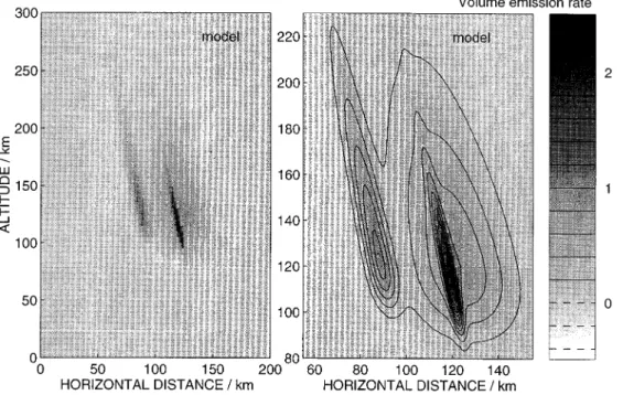
The three instruments in the above example are very far apart. It is obvious that the information for resolving the thin arcs is mainly provided by the middle site, the other two sites mainly contributing to the altitude and vertical profile of the structure. A better horizontal resolu-tion is expected if the instruments are closer to each other and below the auroral structures. Results from such a case are shown in Fig. 5, where three sites at 50, 100 and 150 km are used. The regularisation is the same as in Fig. 4.
A considerable improvement is observed in the results. The thin arcs are now well separated, although still broader than in the model, and the broad diffuse arc is rather well reproduced. The main differences are that the most intense arc is too weak and lies at too high an altitude, and the orientation of the second thin arc is slightly too steep.
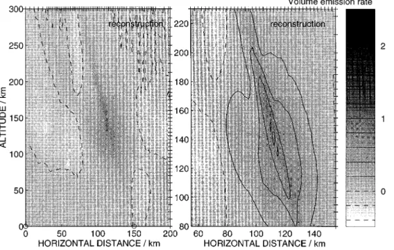
Figure 6 shows results from a set-up which is similar to that in Fig. 5, but in which the three instruments are moved by 25 km to the right. In this reconstruction the orientation of the arc on the left-hand side is now correct, but the other thin arc is almost vertical and much too broad. These examples indicate that the inversion result is rather sensitive to the locations of the instruments.
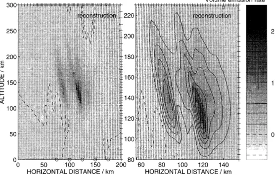
In all cases studied above, the separation of the instru-ments is larger than the distance of the arcs. Results from a case where the opposite is true are shown in Fig. 7, where five instruments are located at distances of 25 km below the auroral structure. Both thin arcs are now cor-rectly oriented and the left-hand one is very well repro-duced. The intensity of the second arc is also much im-proved, although it is still too low. The most obvious deviation from the model is that a vertical bulge has appeared in the diffuse arc, as if a part of the emission rate belonging to the overlaying thin arc would be distributed in the vertical direction.
Altogether, these simulations demonstrate the possibil-ities of the auroral tomographic method in reproducing the volume emission rate in auroral structures. The relia-bility of the results may be limited by the small number of and large distances between the available instruments, as well as the exact location of the auroral arcs with respect to the observation points. It is obvious that a single thin arc is best resolved if one of the instruments lies close to the foot point of the geomagnetic field line of the arc. This fact is also clearly seen in the above examples; in Fig. 5, for instance, the instrument at 150 km has an almost direct
Fig. 5. Same as Fig. 4 for three receivers at 50, 100 and 150 km
Fig. 6. Same as Fig. 4 for three receivers at 75, 125 and 175 km
view along the most intense arc, which is reconstructed remarkably well, whereas the second arc has no instru-ments close to its footpoint and is more poorly repro-duced; in Fig. 6 the instruments are shifted, and the rela-tive quality of the two reconstructed arcs is interchanged.
4 Inversion of auroral camera observations
Because no suitable chain of scanning photometers was available, an effort was made to use auroral TV-camera
observations for testing the method with real data. Even in this case the practical limitations were severe; only two cameras separated by about 200 km were on hand. The cameras were located in Tromsø and Esrange in northern Norway and Sweden, respectively. Based on the above simulations it is obvious that only arcs close to one of the sites can be properly resolved with this sort of experi-mental set-up, and therefore TV frames were selected showing an intense auroral arc in the vicinity of Tromsø. The southernmost camera at Esrange is pointed to the north with a low elevation angle, and the Tromsø camera
Fig. 7. Same as Fig. 4 for five receivers at 75, 100, 125, 150 and 175 km
Fig. 8. Auroral intensity as a function of elevation angle as observed at Tromsø and Esrange at 1959:40 and 200:00 UT on 19 January 1993. The vertical axis is in arbitrary units and the observa-tions from the two sites are in different scales. The elevation angle is defined to be zero for northward horizontal direction and 180° southward horizontal direction in the vertical plane connecting the two sites
is tilted slightly southwards. Hence their common field of view covers a region above and to the south of Tromsø. Because of their low dynamic range (the signal is digitised with 8 bits only), the cameras have an automatic gain control. Therefore, the relative scales of the observations from the two sites vary continuously and there is no method of proper calibration. One might think that this ruins all possibility of using the data in auroral tomogra-phy, but, as shown by the results below this is not quite true. The reason is that the imbalance of the two data sets can be compensated for by the appearance of non-phys-ical negative areas outside the arc region. The result is that at least the location of the arc can be determined.
Figure 8 contains two sets of observations taken from TV frames at the two sites. The curves are signals from lines passing through the local zenith and the second site. The vertical axis is intensity in arbitrary units,
not the same for different sites and times. The horizontal axis is elevation angle with zero value corresponding to horizontal direction to the northern side, 90° to vertical direction and 180° to horizontal direction to the southern side. The Esrange data is taken at elevation angles 6.5°— 51.5° and the Tromsø data at angles 71.7°—128.6°.
Both data sets from Esrange offer a side view of an auroral arc as seen from a long distance. The steep growth as a function of increasing elevation angle is associated with the bottomside of an auroral arc, and the subsequent decrease with the diminishing of the auroral luminosity with altitude. Hence these data contain height informa-tion for the inversion. Informainforma-tion on horizontal variainforma-tion of luminosity is provided by the Tromsø data. In both cases a pronounced maximum is visible at elevation angles greater than 100°, i.e. to the south of the observing site.
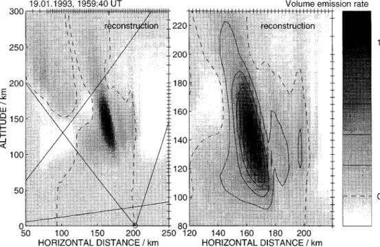
Fig. 9. Volume emission rate reconstructed from the data in Fig. 8 at 1959:40 UT. The sites are shown as dots on the horizontal axis of the
left-hand panel with Esrange at
0 km and Tromsø at 203 km. The viewing angles are shown by the straight lines. The units are arbitrary
Fig. 10. Same as Fig. 9 at 2000:00 UT
Results of tomographic analysis of the two cases are portrayed in Figs. 9 and 10. In the inversion, the same regularisation profile was used as in the previous simula-tions, but without horizontal weighting. The dots on the horizontal axis of the left-hand panels show the locations of the cameras, and the straight lines indicate their fields of view.
It is readily seen that the Esrange camera is too strongly titled to the north, so that it does not see the upper part of the arc, and also the common view of the
cameras is very narrow. In spite of all these limitations, a clear auroral arc is reconstructed slightly to the south of Tromsø. The location of the arcs is the same in both cases, which are separated only by 20 s in time. The fact that negative regions around the arcs appear is not surprising in view of the above simulations and the uncertainties in the data calibration. The tilt angle of the arcs, as determined from the two results, is 77°—78°, which corresponds well to the local magnetic inclination. The peak altitude of the arc is 140—150 km,
i.e. much higher than the peak of the regularisation profile.
In order to test the effect which the uncertainty of the intensity scales may have on the results, several inversions were made by varying the relative scales of the Tromsø and Esrange data sets within wide limits. It turned out that the locations, tilt angles and altitudes of the arcs did not change appreciably; the only variations were in the absolute values of the volume emission rates and the sizes and depths of the negative regions surrounding the arcs. This seems to indicate that, in spite of the defects in the data, the main features of the arcs are correctly recon-structed.
5 Discussion
The most common inversion methods used in ionospheric or auroral tomography are iterative algorithms such as ART and MART. These algorithms begin from a chosen start distribution and vary it in the direction guided by the observations until either the results no longer change or a least-square minimum is achieved. The iteration works very much on an intuitive level, and, as pointed out by Censor (1983), it is not well understood how good the results are. It is not necessarily clear whether the iteration converges at all, and if it does, it is not known how close to the convergence limit the iteration has stopped. Further-more, depending on the start distribution, the iteration may lead to different results which all satisfy the original measurements equally well. It seems probable that the iteration leads to a correct result, if the start profile is close enough to the true distribution. This is especially impor-tant in ionospheric tomography, where the horizontal gradients are often small and the measurements contain only little information on the profile shape. Therefore much effort has been put in choosing the start profiles in ionospheric tomography. In auroral tomography the tar-get is usually limited in horizontal direction, and therefore the start profile is probably less important: it seems that the iteration can even be put to start from a constant function (Vallance-Jones et al., 1991).
Stochastic inversion greatly differs from all iterative methods. The most important difference is that stochastic inversion has a firm mathematical background. Therefore it is well understood what the result actually is: it simply gives the most probable values of the unknowns once the measurements are known and the regularisation is fixed. The effect of measurement errors is also included in the formalism. The result is obtained after a single inversion, and no start profiles or stop criteria are needed, which are essential in iterative methods.
An important part of stochastic inversion is regularisa-tion which prevents non-physical point-to-point oscilla-tions otherwise created by the numerical instability in matrix inversion. In the present method, regularisation is also used in feeding the solver by a priori information on the volume emission rate or electron density. It is essential to understand that the regularisation by no means deter-mines the shape or altitude of the resulting profile. This is clearly observed in Figs. 9 and 10, where the peaks of the
auroral arcs are at 140—150-km altitudes, although the peak height of the regularisation profile is 120 km. Al-though not always understood by the users, the iterative algorithms also take advantage of a priori information contained in the start profile and stop criteria. The differ-ence is, however, that in stochastic inversion the a priori information has a well-defined role in the formalism, whereas in iterative algorithms its effect is difficult to quantify.
Although stochastic inversion has a more solid theoret-ical background than various iterative methods, this does not necessarily mean that the latter would give worse results. Depending on the dimensions and location of the target, as well as the selected start distribution, the iter-ative algorithms may lead to equally good results. Fur-thermore, if the regularisation variances are not well chosen, the results given by stochastic inversion may even be worse. It would be interesting to make a comparison of the two types of methods using blind tests with simulated data. This would imply cooperation of different tomogra-phy groups.
The software used in the present work was originally developed for ionospheric tomography. Therefore the grid is horizontal and the regularisation variances are given for vertical and horizontal steps of the volume emission rate or electron density. The sort of regularisation can be used to make the inversion routine interpret the observations in terms of horizontal or vertical structures. In the present work the vertical variances are smaller than the horizontal ones, and then, if at all possible, the software tries to twist the arcs into a vertical position. This tendency is clearly seen in the above simulation examples. Therefore, al-though suitable in ionospheric tomography, the regular-isation method is less appropriate in studying auroral arcs which are aligned along the geomagnetic field. The most straightforward way of modifying the programme for aur-oral tomography would be to tilt the grid according to the local inclination. Then one could give smaller regularisa-tion variances in the direcregularisa-tion of the arc than in the perpendicular direction, and the solution would favour field-aligned structures instead of vertical ones.
The next task is to modify the analysis programme for auroral work according to the above guideline. A more extensive project would be to include the possibility of three-dimensional tomography. Although there would be no change in the general principles, the part of the pack-age involving the experimental geometry should be com-pletely revised. The inversion problem would be much bigger than in a two-dimensional case of course, and probably such a high spatial resolution could not be used as in the present work.
Altogether, auroral tomography seems to be a very promising new field which has not yet been utilised or developed to its full power. All its benefits will not be obtained merely by the development of inversion methods and analysis programmes, but it is essential that data of good quality be available from a dense enough network of optical instruments.
Acknowledgements. The work done by P. Henelius and E. Vilenius
in programme development is gratefully acknowledged.
Topical Editor D. Alcayde´ thanks I. Pryse and A. Vallance-Jones for their help in evaluating this paper.
References
Aso, T., and M. Ejiri, CAT — a method for the determination of aurora luminosity structures, in ¹he 19th Annual European
Meeting on Atmospheric Studies by Optical Methods, August
10—14, 1992, Kiruna, Sweden, IRF Scientific Report 209, 249—254, 1992.
Aso, T., T. Hashimoto, M. Abe, T. Ono, and M. Ejiri, On the Analysis of Aurora Stereo Observations, J. Geomagn. Geoelectr., 42, 579—595, 1990.
Censor, Y., Finite Series-Expansion Reconstruction methods, Proc.
IEEE, 71, 409—419, 1983.
Fehmers, G., A new algorithm for ionospheric tomography, in
Proceedings of the International Beacon Satellite Symposium, ºni-versity of ¼ales, Aberystwyth, ºK, 11–15 July 1994 (Ed. L.
Kersley), 52—55, 1994.
Fremouw, E. J., J. A. Secan, and B. M. Howe, Application of stochastic inverse theory to ionospheric tomography, Radio Sci., 27, 721—732, 1992.
Gordon, R., Industrial applications of computed tomography and NMR imaging: an OSA Topical Meeting, Appl. Opt., 24, 3948—3949, 1985.
Gustavsson, M., S. Ivansson, P. More´n, and J. Pihl, Seismic borehole tomography — measurement system and field studies, Proc.
IEEE, 74, 339—346, 1986.
McDade, I. C., and E. J. Llewellyn, Inversion techniques for recover-ing two-dimensional distributions of auroral emission rates from tomographic rocket photometer measurements, Can. J. Phys., 69, 1059—1068, 1991.
McDade, I. C., N. D. Lloyd, and E. J. Llewellyn, A rocket tomogra-phy measurement of the N`2 3914 As emission rates within an auroral arc, Planet. Space Sci., 39, 895—906, 1991.
Markkanen, M., M. Lehtinen, T. Nygre´n, J. Pirttila~ , P. Henelius, E. Vilenius, E. D. Tereshchenko, and B. Z. Khudukon, Bayesian approach to satellite radiotomography with applications in the Scandinavian sector, Ann. Geophysicae, 13, 1277—1287, 1995. Munk, W., and C. Wunsch, Ocean acoustic tomography: a scheme
for large scale monitoring, Deep Sea Res., 26A, 123—161, 1979. Pryse, S. E., and L. Kersley, A preliminary experimental test of
ionospheric tomography, J. Atmos. ¹err. Phys., 54, 1007—1012, 1992.
Solomon, S. C., P. B. Hays, and V. J. Abreu, Tomographic inversion of satellite photometry, Appl. Opt., 23, 3409—3414, 1984. Solomon, S. C., P. B. Hays, and V. J. Abreu, Tomographic inversion
of satellite photometry. Part 2, Appl. Opt., 24, 4134—4140, 1985. Takauchi, Y., and J. R. Evans, Teleseismic tomography of the Loma Prieta earthquake region. California: implications for strain par-titioning, Geophys. Res. ¸ett., 22, 2203—2206, 1995.
Vallance-Jones, A., R. L. Gattinger, F. Creutzberg, F. R. Harris, A. G. McNamara, A. W. Yau, E. J. Llewellyn, D. Lummerzheim, M. H. Rees, I. C. McDade, and J. Margot, The ARIES auroral modelling campaign: characterization and modelling of an evening auroral arc observed from a rocket and a ground-based line of meridian scanners, Planet. Space Sci., 39, 1677—1705, 1991.