HAL Id: hal-01216117
https://hal.archives-ouvertes.fr/hal-01216117
Submitted on 16 Oct 2015
HAL is a multi-disciplinary open access
archive for the deposit and dissemination of sci-entific research documents, whether they are pub-lished or not. The documents may come from
L’archive ouverte pluridisciplinaire HAL, est destinée au dépôt et à la diffusion de documents scientifiques de niveau recherche, publiés ou non, émanant des établissements d’enseignement et de
Time-dependent wave splitting and source separation
Marcus Grote, Marie Kray, Frédéric Nataf, Franck Assous
To cite this version:
Marcus Grote, Marie Kray, Frédéric Nataf, Franck Assous. Time-dependent wave splitting and source separation. Journal of Computational Physics, Elsevier, 2017, 330, pp.981-996. �10.1016/j.jcp.2016.10.021�. �hal-01216117�
Time-dependent wave splitting and source separation
Marcus J. Grote
a, Marie Kray
a, Frédéric Nataf
b,c,d, Franck Assous
e a Department of Mathematics and Computer Science, University of Basel, Spiegelgasse 1,CH-4051 Basel, Switzerland, {marcus.grote,marie.kray}@unibas.ch b CNRS, UMR 7598, Laboratoire Jacques-Louis Lions, F-75005, Paris, France c UPMC Univ Paris 06, UMR 7598, Laboratoire Jacques-Louis Lions, F-75005, Paris,
France, [email protected]
dINRIA Rocquencourt, Alpines, BP 105, 78153 Le Chesnay Cedex, France e Department of Mathematics, Ariel University, 40700, Ariel, Israel,
Abstract
Starting from classical absorbing boundary conditions, we propose a method for the separation of time-dependent scattered wave fields due to multiple sources or obstacles. In contrast to previous techniques, our method is local in space and time, deterministic, and also avoids a priori assumptions on the frequency spectrum of the signal. Numerical examples in two space dimen-sions illustrate the usefulness of wave splitting for time-dependent scattering problems.
Keywords:
Time-dependent scattering, wave splitting, source separation, absorbing bound-ary conditions
1. Introduction
As natural information carriers, acoustic, electromagnetic and elastic waves are ubiquitous for probing an unknown medium to determine its in-ternal geometric or material properties. When the incident probing wave encounters an inhomogeneity, it generates a scattered wave which carries information about the obstacle across the background medium. From that scattering data, usually recorded at remote sensors, the nature, location and shape of the obstacle buried inside the medium can be recovered, as in seis-mic full waveform inversion, medical imaging, and nondestructive testing. Clearly, that information is readily available by subtraction of the incident
wave from total field measurements. However, if the location, spatial distri-bution or time dependence of the original source are not precisely known, or other undesired sources interfere with the signal, extraction of the scat-tered field of interest becomes non-trivial, though it remains essential for any subsequent inversion.
Blind source separation in signal processing [6], for instance, attempts to separate the input signals from their recorded mixture, much like in the well-known ”cocktail-party e↵ect” where listeners perceptually focus on a single target voice against competing sound sources. Ray-based in nature, blind source separation uses statistical tools to detect individual sources [8] or remove noise [2] from linearly superimposed signals.
In transcranial ultrasonic imaging, intense ultrasound pulses induce a single cavitation bubble whose collapse generates a small shock wave then recorded by a standard ultrasound imaging array [22]; clearly, the bubble’s time signature is never precisely known. Similarly, the detection of individ-ual free-floating and targeted microbubbles of an ultrasound contrast agent is critical for quantifying the amount of bubbles in the tissue [20]. Yet an-other application is photoacoustic imaging, where laser pulses are delivered into biological tissues thereby leading to transient thermoelastic expansion and subsequent ultrasonic emission. Again, the quantity of interest is the time signature of the laser induced pressure wave generated by an unknown source [25].
When two or more obstacles are present, each primary scattered wave will induce secondary scattered waves from all other obstacles, which again will induce further scattered waves, and so forth. Together with the incident wave, their superposition results in the measured total wave field. The inver-sion from the total wave field for multiple obstacles at once adds yet another layer of complexity to any algorithm for inverse scattering problems. Hence, if their superposition can be split into individual outgoing components, we can apply any algorithm for single inverse scattering to each scatterer sepa-rately. As a consequence, each isolated scattering problem will be smaller in size and less ill-conditioned than their total sum.
In seismic imaging, for instance, shear-wave splitting has been successfully used for earthquake prediction or in the petroleum industry. Indeed when a polarized elastic shear wave enters a new, anisotropic medium, it splits into two shear waves whose mutual time-delay and orientation then allows to infer the density and orientation of the cracks in the medium. In [21], Kreider uses Weston’s theoretical wave splitting for stratified media [27] to reconstruct
the unknown velocity function in a stratified inhomogeneous cylinder from reflection data.
There is a long history of wave splitting techniques for multiple scat-tering problems, especially in the frequency domain. In his classical work, Twerksy expresses multiple scattering coefficients in terms of algebraic rela-tions which couple the multipole coefficients of isolated scatterers – see [26] for a review. More recently, Grote and Kirsch [12] used wave splitting to derive nonreflecting boundary conditions for multiple scattering problems. Similarly, Acosta [1] formulated on-surface radiation conditions for multiple scattering. In [7], Ben Hassen, Liu and Potthast split the far-field pattern us-ing integral based formulations to extend the point source method to inverse scattering of multiple obstacles. By combining the inverse Radon approxima-tion with a Galerkin ansatz, Griesmaier, Hanke and Sylvester determine the convex scattering support of individual far-field components separately [10]. In the time domain, little work on inverse multiple scattering problems is available. In [13, 15], nonreflecting boundary conditions for time-dependent multiple scattering were derived, which avoid the space-time integrals in-volved in standard integral-based formulations. By Fourier transform in the frequency domain, Potthast, Fazi and Nelson [23] devised a filter via the point source method for time-dependent source separation.
Here we propose a method to determine the separate outgoing compo-nents of the incident and scattered wave fields for time-dependent scattering problems. In contrast to previous work, our approach is local in space and time, deterministic, and also avoids any a priori assumptions on the fre-quency spectrum of the signal. Starting from the standard Bayliss-Turkel [5] absorbing boundary conditions, we present in Section 2 the principle of wave splitting, first introduced in [14], which we then illustrate in the simpler one-dimensional case. Next, in Section 3, we present our wave splitting approach in the general two-dimensional case and also discuss its numerical implemen-tation. Finally, in Section 4, we consider two distinct numerical experiments to illustrate the usefulness of our wave splitting approach.
2. Wave splitting
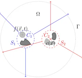
We consider wave scattering from two distinct scatterers, which each may contain several obstacles, inhomogeneities and nonlinearity. Both scatterers are well separated, that is we assume that we can surround them by two non-intersecting spheres S1 and S2 centered at C1 and C2, respectively –
see Fig. 1. In ⌦, the unbounded domain outside S1 and S2, the scattered wave field u satisfies:
@2u @t2 c
2 u = 0 in ⌦, t > 0, (1) with constant wave speed c > 0. Moreover, we assume that u is initially confined to the interior of S1[S2; thus, it is zero throughout ⌦ at time t = 0. Then u splits into two unique wave fields u1 and u2 as
u = u1 + u2 in ⌦, t > 0, (2) where each uk is purely outgoing and satisfies (1) in the entire exterior of Sk [13]; hence, uk is determined by its time-dependent (unknown) val-ues on Sk, k = 1, 2.
Since each uk is outgoing outside Sk, it can be written as a progressive wave expansion in inverse powers of distance [5, 16] from Ck. In three space dimensions, for instance, we have
uk(t, rk, ✓k, 'k) = 1 rk X i 0 fk,i(rk ct, ✓k, 'k) (rk)i , (3)
where (rk, ✓k, 'k) denote spherical coordinates centered about the origin Ck, k = 1, 2. In two space dimensions, the progressive wave expansion of uk converges only asymptotically:
uk(t, rk, ✓k) ⇠ p1rkX i 0
fk,i(rk ct, ✓k)
(rk)i , rk ! 1, (4) where (rk, ✓k) denote polar coordinates centered about the origin Ck, k = 1, 2. Starting from (3), (4) respectively, Bayliss and Turkel [5] derived a se-quence of increasingly accurate di↵erential operators of order m that annihi-late the m leading order terms in either expansion above for k = 1, 2:
Bkm[uk] := m Y `=1 ✓ 1 c @ @t+ @ @rk + 2` 1 rk ◆ = O ✓ 1 r2m+1k ◆ , ⌦⇢ R3, (5) Bkm[uk] := m Y `=1 ✓ 1 c @ @t+ @ @rk + 4` 3 2rk ◆ = O 1 r2m+12 k ! , ⌦⇢ R2.(6)
⌦ S1 ⇥ C1 . f (~x, t) S2 ⇥ C2 c(~x)
Figure 1: Two distinct scatterers and their corresponding outgoing wave fields.
By setting
Bkm[uk] = 0, (7)
each operator yields an absorbing boundary condition on any (convex) surface patch in three dimensions or curve segment in two dimensions.
Now, let denote a surface patch or curve segment, not necessarily closed or connected, which lies inside ⌦. Neglecting the error term in (5)-(6), we thus obtain on
Bjm[uk] = Bjm[uk+ uj] = Bjm[u], j = 1, 2, k 6= j. (8) When u is known on , equation (8) yields a partial di↵erential equation for the unknown wave field uk. In general, it will involve tangential, normal and time derivatives. To restrict (8) to , we rewrite the normal derivative (@rj)
as a combination of tangential and radial (@rk and @✓k) derivatives and then
replace radial by time derivatives using (3) or (4), respectively. The result-ing equation will involve only tangential and time derivatives and thus be restricted to . Clearly, appropriate initial and boundary conditions must be set on for well-posedness. In fact, since the scattered field is initially zero in ⌦, both uk and uj vanish on at t = 0.
Remark 2.1. In (8), the absorbing di↵erential operator Bm
j enables the re-covery of every outgoing component of the total field into ⌦ in forward time. Instead, we can also consider time-reversed wave fields propagating backwards
in time. By replacing the coupled space-time variable rk ct by rk+ ct in the progressive wave expansions (3),(4), we thus obtain di↵erential operators which instead annihilate incoming wave fields.
In the three-dimensional case, for instance, let Bj = B1
j denote the first-order Bayliss-Turkel operator:
Bj[u] = ✓ 1 c @ @t + @ @rj + 1 rj ◆ u. (9)
Then, the new operator for the time-reversed total field, uR, reads: BR,j[uR] = ✓ 1 c @ @t @ @rj 1 rj ◆ uR. (10)
Thus, it is possible to extend wave-splitting even to parts of , where the forward problem (8) may be ill-posed. To use this time reversed operator, however, we must also set an initial condition for uR,k or uR,j at the final time t = T . If T is sufficiently large so that the total wave field has entirely left ⌦, we can simply set uR,k and uR,j to zero at time t = T as initial condition for wave splitting in time reversal. ⌅ 2.1. One-dimensional wave splitting
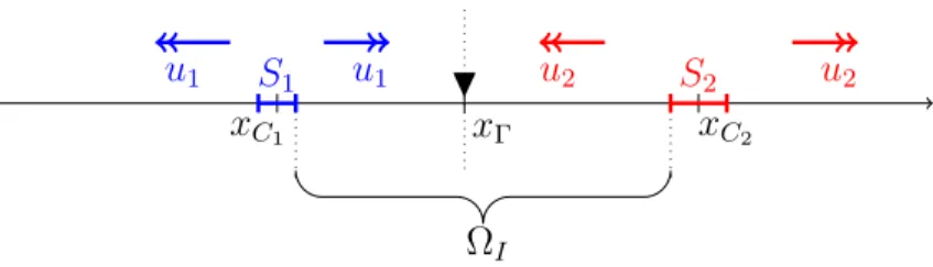
Before proceeding with the higher dimensional case, we briefly consider the much simpler one-dimensional situation to illustrate the basic principle of wave splitting. Hence we consider two sources located inside of two disjoint intervals S1 and S2, separated by an interval ⌦I – see Fig. 2. Now, as waves are excited inside S1 and S2, they propagate into ⌦I where they mingle and form the total wave field u(t, x). Since u is initially zero and the wave speed, c, is assumed constant outside the two scatterers, the total field consists of a right-moving wave, u1, and a left-moving wave, u2:
u(t, x) = u1(x c t) + u2(x + c t), x2 ⌦I, t 0. (11) Next, let x denote an observation point located well inside ⌦I. Given the time history of the total field u(t, x ) at the receiver, we wish to recover the two individual one-way wave fields u1 and u2.
Following the approach delineated in the previous section for the two- or three-dimensional case, we consider the one-way di↵erential operators
B1[u] := @u @t + c @u @x, B2[u] := @u @t c @u @x. (12)
x H ⌦I xC1 u1 u1 xC2 u2 u2 S1 S2
Figure 2: One-dimensional wave splitting. The receiver is located at x .
Since B1[u1] = B2[u2] = 0, we thus obtain the one-dimensional counterpart of (8) inside ⌦I:
B1[u2] = B1[u1] + B1[u2] = B1[u], (13) B2[u1] = B2[u1] + B2[u2] = B2[u]. (14) Hence, equations (13),(14) correspond to partial di↵erential equations for the unknown wave fields u1, u2 which both involve derivatives in space and time. Since B2[u2] = 0 inside ⌦I, we can replace in (13) the space by the time derivative of u2, and similarly for u1 in (14):
B1[u2] = @u2 @t + c @u2 @x = 2 @u2 @t , B2[u1] = @u1 @t c @u1 @x = 2 @u1 @t .
Setting x = x in the resulting equations, we obtain the two ordinary equa-tions: @u2 @t (x + c t) = 1 2B1[u](t, x ), (15) @u1 @t (x c t) = 1 2B2[u](t, x ). (16) To recover u1 or u2, we shall integrate (15) and (16) in time, together with homogeneous initial conditions, since the signal at x is initially zero. Here, we opt for the Crank-Nicolson scheme and let un
2 ' u2(x + c tn), un
1 ' u1(x c tn) denote the numerical approximations at time tn = n t, t > 0. The discrete time-marching scheme then reads:
un+12 = un2 + t 4 B1[u](t n+1, x ) + B1[u](tn, x ) , n 0, (17) un+11 = un1 + t 4 B2[u](t n+1, x ) + B2[u](tn, x ) , n 0, (18)
−10 −8 −6 −4 −2 0 2 4 6 8 10 0 1 2 3 4 5 6 x u 1 u 2 u total
Figure 3: One-dimensional wave splitting. Snapshot of the total field u with the right-and left-propagating waves u1 and u2 at time t = 7.45. The two receivers are located at x = 2 and x = 4.4 (vertical dashed lines).
and u0
2 = 0, u01 = 0. The right-hand-side is discretized using centered finite di↵erences in time and in space in our simulation, assuming we know u in a small neighborhood of x .
For illustration, we consider a numerical experiment with c = 1 and the two intervals S1 = [ 8, 3], S2 = [5, 12] centered about xC1 = 5.5,
xC2 = 8.5, respectively. Inside each interval, we initialize a Gaussian-like
wave
u1(x, t) = e ((x xC1) ct)4 S
1(x), u2(x, t) = 5e
((x xC2)+ct)2
S2(x),
where S denotes the characteristic function of S. Hence the total field, u(x, t) = e ((x xC1) ct)4 S
1(x) + 5e
((x xC2)+ct)2
S2(x),
is identically zero at t = 0 inside ⌦I.
In Fig. 3, we display a snapshot of the total field u(t, x) at time t = 7.45 together with the right- and left-propagating waves u1 and u2 that we wish to recover. For the reconstruction of u1 and u2, we consider two distinct locations: x = 2 and x = 4.4. At x = 4.4, u1 and u2 can easily be sepa-rated because of their very di↵erent arrival times – see left column of Fig. 4.
0 5 10 15 20 0 5 t u total 0 5 10 15 20 0 5 t u 1 reconstr. u 1 exact 0 5 10 15 20 0 5 t u 2 reconstr. u 2 exact 0 5 10 15 20 0 5 t u total 0 5 10 15 20 0 5 t u 1 reconstr. u 1 exact 0 5 10 15 20 0 5 t u 2 reconstr. u 2 exact
Figure 4: One-dimensional wave splitting. Reconstruction of the time history of u1 and u2 at x = 4.4 (left column) and x = 2 (right column) from the total field u using (18) and (17).
At x = 2, however, the two fields are completely superimposed and thus difficult to separate by eye-ball only – see right column of Fig. 4. In either case, our approach allows us to recover the full time history of u1 and u2 at the receiver’s location with high accuracy.
For simplicity, here the considered wave speed c is constant everywhere; hence, the exact wave fields u1, u2 and u are readily available. Our wave split-ting approach, however, also immediately applies to the situation when c(x) varies inside S1 and S2.
3. Two-dimensional case
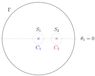
We shall now apply the wave splitting technique delineated in Section 2 to a typical two-dimensional configuration. Hence, we assume that the total field u is recorded on a circle centered at either of the two sources C1 or C2. Given the measured values of u on , here a circle centered about C1 – see Fig. 5 – we shall recover both outgoing fields u1 and u2 using first-order absorbing di↵erential operators.
✓1 = 0 ⇥ C1 S1 ⇥ C2 S2
Figure 5: The two sources are located inside S1 and S2, while the measurements are located on the circle , centered at C1.
3.1. Recovery of u1
First, we shall show how to recover u1 on from u. Let (rk, ✓k) denote polar coordinates centered at Ck, k = 1, 2. Now, let the ✓1 = 0 axis coincide with the line segment connecting C1 and C2, which is always possible by rotating the coordinate system. Following the derivation in Section 2, we apply B2 := B1
2 from (6) to the measured total field u, which yields the two-dimensional counterpart of (8): ✓ 1 c @ @t+ @ @r2 + 1 2r2 ◆ u1 = ✓ 1 c @ @t+ @ @r2 + 1 2r2 ◆ u. (19) To restrict equation (19) for u1 to , we first change coordinates and then replace any remaining normal by time derivatives using that B1[u1] = 0. More specifically, we use
@ @r2 = r2+ ` cos(✓2) r1 @ @r1 + ` sin(✓2) r2 1 @ @✓1 (20) @ @r1( p r1u1) = 1 c @ @t( p r1u1), (21)
with ` the distance between C1 and C2, to rewrite (19) for the leading order term f1 := f1,0(r1 ct, ✓1) of the series expansion in (4) as
✓ ↵1(✓1)@ @t + 1(✓1) @ @✓1 + 1(✓1) ◆ f1 = ✓ 1 c @ @t+ @ @r2 + 1 2r2 ◆ u. (22)
Here, the coefficient functions ↵1, 1 and 1 in (22) are given by ↵1(✓1) = p r2 1 + `2 2r1` cos(✓1) r1+ ` cos(✓1) cpr1 p r2 1+ `2 2r1` cos(✓1) , (23) 1(✓1) = ` sin(✓1) r1pr1pr2 1 + `2 2r1` cos(✓1) , (24) 1(✓1) = ` cos(✓1) 2r1pr1pr2 1 + `2 2r1` cos(✓1) . (25)
Note that both ` and r1 are constant on , while r2
1 + `2 2r1` cos(✓1) > 0, 8 ✓1 2 [ ⇡, ⇡].
In (22), we have derived a partial di↵erential equation for f1(r1 ct, ✓1), which only involves time and space derivatives of f1 tangential to . To determine the domain of validity and the well-posedness of the hyperbolic equation (22), we now study the sign of each coefficient, which determines the directions of the characteristics and thus dictates the appropriate boundary conditions, if any, needed. As initial condition, we set u1 to zero on , as u is initially zero inside ⌦.
Since
r21+ `2 2r1` cos(✓1) r12+ `2cos(✓1)2 2r1` cos(✓1) = (r1 ` cos(✓1))2, we have
q r2
1 + `2 2r1` cos(✓1) r1 ` cos(✓1).
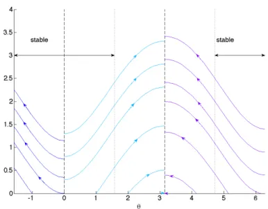
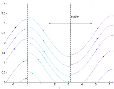
Therefore, ↵1(✓1) 0 for all ✓1 2 [ ⇡, ⇡]; note that ↵1 = 0 for ✓1 = 0, ⇡. We now proceed likewise for 1 and 1. Since ` and r1 are positive, 1 is nonnegative for ✓1 2 [0, ⇡]. For ✓1 = 0, ⇡, 1(✓1) vanishes and hence (22) reduces to a trivial equation (without derivatives) in time. In that sense, both ✓1 = 0, ⇡ are singular points. From (25), we infer that 1 is pos-itive for ✓1 2 ( ⇡/2, ⇡/2), negative for ✓1 2 (⇡/2, 3⇡/2), and vanishes for ✓1 = ⇡/2, ⇡/2. Since (22) is unstable when the signs of 1 and ↵1 do not match, and ↵1(✓1) 0 for all ✓1, we conclude that (22) is stable only for ✓1 2 [ ⇡/2, ⇡/2] – see Fig. 8.
Figure 6: Characteristic curves for (22) starting from di↵erent angles ✓
In Fig. 6, we display the characteristics of (22) and clearly observe two distinguished points: ✓1 = 0 and ✓1 = ⇡. At ✓1 = 0, the characteristics are always incoming and thus ✓1 = 0 yields an appropriate initial condition to recover the signal in both intervals [0, ⇡) and ( ⇡, 0]. On the contrary, ✓1 = ⇡ is never reached by any characteristic (except for that starting from ✓ = ⇡ itself). From these considerations, we impose at ✓1 = 0 a Dirichlet boundary condition to solve (22) in a stable manner on the two independent quarter-circles [0, ⇡/2] and [ ⇡/2, 0].
To determine u1 on the remaining half-circle, ✓1 2 [⇡/2, 3⇡/2], where u1 is exponentially growing, we consider the time-reversed counterpart of (22). Hence, we let uR denote the time-reversed total wave field and apply the time-reversed first-order Bayliss-Turkel operator BR,2 – see Remark 2.1 – which yields: ✓ 1 c @ @t @ @r2 1 2r2 ◆ uR,1= ✓ 1 c @ @t @ @r2 1 2r2 ◆ uR. (26) Following the previous derivation (19)-(22), we replace the normal derivative by tangential and time derivatives in (26) using (20), (21). This yields the time-reversed counterpart of (22) for the leading term, fR,1, in the series
Figure 7: Characteristic curves for (27) starting from di↵erent angles ✓
expansion of the time-reversed wave field: ✓ ↵R,1(✓1)@ @t + R,1(✓1) @ @✓1 + R,1(✓1) ◆ fR,1 = ✓ 1 c @ @t @ @r2 1 2r2 ◆ uR. (27) Here, the coefficient functions are given by
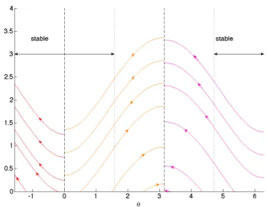
↵R,1(✓1) = ↵1(✓1), R,1(✓1) = 1(✓1), R,1(✓1) = 1(✓1), (28) with ↵1, 1 and 1 as in (23)-(25). Again, ↵R,1and R,1 are zero at ✓1 = 0, ⇡, while ↵R,1is always positive. The sign of R,1is now opposite to that of 1, as confirmed by the direction of the corresponding characteristics – see Fig. 7. Moreover, since R,1 and 1 have also opposite signs, equation (27) is now stable on [⇡/2, 3⇡/2], where both ↵R,1and R,1are nonnegative. According to the direction of the characteristics, we must now set the boundary condition at ✓1 = ⇡.
The initial condition for the time reversed equation (27) is given by the value of u at t = T , where T is the final recording or simulation time. Since it is no longer possible to distinguish u1 from u2 at later times, we must set the final time T sufficiently large so that the total wave field has left the computational domain and thus vanishes throughout ⌦. Hence, we set f1 = 0 at t = T , or fR,1 = 0 at t = 0, equivalently.
⇥ ⇥ C1 C2
✓1 = 0
✓1 = ⇡ equation (22)solve forward solve TR
equation (27)
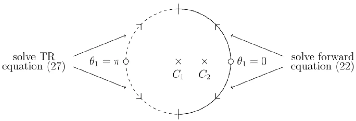
Figure 8: The domain of validity for the recovery of f1 and fR,1. Plain line: solve the forward equation (22). Dashed line: solve the time-reversed (TR) equation (27). The characteristics point away from the two small circles at ✓1 = 0, ⇡, where the boundary conditions are set, towards the vertical bars at ✓1 = ⇡/2, ⇡/2, which mark the end of validity of each quarter-circle.
Finally, we recover u1 by solving (22) on [ ⇡/2, 0[S]0, ⇡/2] forward in time and (27) backward in time on [⇡/2, ⇡[S]⇡, 3⇡/2], as shown in Fig. 8. In pratice, due to the two dividing characteristics at ✓1 = 0, ⇡, we actually solve four partial di↵erential equations on four quarter-circles independently of each other. Since (22) and (27) both involve only partial derivatives but no integrals, our approach is local in time and in space. In fact, to reconstruct the signal at any fixed point P at some time t0 > 0, we need to know the total field only on the fraction of the circle from ✓1 = 0 to P , or from ✓1 = ⇡ to P , respectively, and for t 2 [0, t0].
Note that in the special case when u1 or u2 corresponds to a purely radial wave generated by a point source, the corresponding partial di↵erential equation (22) or (27) reduces to an ordinary di↵erential equation, which can be solved for any particular angle independently, regardless of the shape of ⌦. 3.2. Recovery of u2
In the previous section, we derived equations (22) and (27) to recover u1 on the entire circle . From the recorded data u, we can thus simply recover u2 by subtraction. However, we can also recover u2 from a new independent equation by applying B1 := B1 1 from (6) instead of B2 to u: ✓ 1 c @ @t+ @ @r1 + 1 2r1 ◆ u2 = ✓ 1 c @ @t+ @ @r1 + 1 2r1 ◆ u. (29)
Figure 9: Characteristic curves for (31) starting from di↵erent angles ✓
Again, we use (20) to replace the radial derivative on the left of (29) by a combination of radial and tangential derivatives. Next, we use (7) with m = 1 and k = 2, that is @ @r2( p r2u2) = 1 c @ @t( p r2u2), (30)
to replace the remaining radial derivative by a time derivative. Thus, we obtain the following partial di↵erential equation for the leading order term f2 := f2,0(r2 ct, ✓2) in the series expansion (4) of u2:
✓ ↵2(✓1)@ @t + 2(✓1) @ @✓1 + 2(✓1) ◆ f2 = ✓ 1 c @ @t+ @ @r1 + 1 2r1 ◆ u. (31) Here, the coefficient functions are given by
↵2(✓1) = p r2 1+ `2 2r1` cos(✓1) r1+ ` cos(✓1) cp4 r2 1+ `2 2r1` cos(✓1)(r1 ` cos(✓1)) , 2(✓1) = ` sin(✓1) r1p4 r2 1 + `2 2r1` cos(✓1)(r1 ` cos(✓1)) , 2(✓1) = 1 2p4 r2 1 + `2 2r1` cos(✓1)(r1 ` cos(✓1)) ✓ ` cos(✓1) r1 `2sin(✓1)2 r2 1+ `2 2r1` cos(✓1) ◆ .
Note that ↵2, 2 and 2 are still functions of ✓1, since we recover u2 on the circle still centered at C1. Remarkably, the signs of ↵2, 2 and 2 coincide with those of ↵1, 1and 1, respectively, and so do the characteristics curves – see Fig. 9. Therefore, the same conclusions hold about the initial condition, the boundary conditions at ✓1 = 0, ⇡, and the stability properties of (31) on [ ⇡/2, 0)[(0, ⇡/2]. Similarly, we use the time reversed counterpart of (31), which is omitted here, to reconstructed u2 on [⇡/2, ⇡)[ (⇡, 3⇡/2] – see Fig. 8.
3.3. Numerical discretization
To determine u1 on , we shall solve (22) or (27) numerically, depending on the quarter-circle considered. For the numerical discretization, we opt for the standard Crank-Nicolson scheme in time and upwinding finite di↵erences in space following the characteristics. The numerical discretization of (27) on ⇥⇡
2, ⇡ , for instance, reads: ↵(i ✓)f n+1 i fin t + 1 2 (i ✓) ✓fn+1 i+1 fin+1 ✓ + fn i+1 fin ✓ ◆ + 1 2 (i ✓) f n+1 i + fin = 1 2 g n+1 i + gin , (32) with gn i = BR,2[u](tn, i ✓) and f10 ⌘ 0 at t = 0. To compute the right-hand-side gn
i = BR,2[u](tn, i ✓) in (27), the wave field u and its radial derivative are both computed with the finite element software FreeFem++ [18]. Indeed, from the variational formulation, we easily get an accurate approximation of the radial derivative at , since
Z @u @rjv = Z @u @nv = ZZ ⌦ @2u @t2w + ZZ ⌦ ru · rw . (33) Here, denotes a circle centered at Cj, while w 2 H1(⌦) is an extension of the trace v 2 H12( ) into ⌦, which vanishes on all vertices inside ⌦. For
the time and tangential derivatives, we use finite di↵erences and cubic spline interpolation. As the numerical discretizations used on the left and right side of (32) di↵er, we also avoid any potential “inverse crime”.
4. Numerical examples
To illustrate the usefulness of the wave splitting approach described in Section 3, we now consider numerical experiments in two di↵erent geometric configurations.
4.1. Two point sources
First, we consider two point sources F1(t) and F2(t), located at C1and C2 – see Fig. 1. Each source generates an outgoing wave field uj. At the outer boundary, we record their sum: u = u1+ u2. Given that observed data on , we wish to recover the two separate components u1 and u2. Hence, u satifies the wave equation
@2u @t2 c
2 u = F1(t)
x=C1 + F2(t) x=C2, inR
2, (34) with homogeneous initial conditions. The time dependence of the two sources F1 and F2, shown in Fig. 10, is given by
Figure 10: Time dependence of the two point sources F1 and F2 in (34).
F1(t) = [1 2⇡2(⌫(t d1) 1)2] e ⇡ 2(⌫(t d 1) 1)2 3 2[1 2⇡ 2(2⌫(t d2) 1)2] e ⇡2(2⌫(t d 2) 1)2 3 5⇡ 2(⌫(t d3) 1)e ⇡2(⌫(t d 3) 1)2, (35) F2(t) = 1 2[1 2⇡ 2(⌫(t d1) 1)2] e ⇡2(⌫(t d1) 1)2 +2 [1 2⇡2(2⌫(t d 2) 1)2] e ⇡ 2(2⌫(t d 2) 1)2 1 4⇡ 2(⌫(t d3) 1)e ⇡2(⌫(t d3) 1)2 (36)
Figure 11: Two point sources. Snapshot of the total wave field at t = 0.64.
with d1 = 0.01, d2 = 0.41, d3 = 0.61 and ⌫ = 5. They consist of the superposition of three time shifted Ricker-like sources. Next, we set c ⌘ 1, the wavelength = 0.2 and let C1 and C2 equal ( /2, 0) and ( /2, 0), respectively. The total field is recorded on a circle centered at C1 with radius 5 /2 – see Fig. 11.
In Fig. 12, we display the time history of the recovered two wave fields u1 and u2 at P1, located on at ✓1 = ⇡/4. Due to the particularly simple set-up, here both u1 and u2 are known explicitly and for all time. In the top left frame, we compare u1, obtained by solving (22), with the exact wave field and observe that both coincide quite well. Similarly, the wave field u2, recovered by solving (31), compares favorably with the exact wave field ema-nating from C2. Then in the top right frame, we compare the sum u1+ u2 of the two recovered fields from (22) and (31), with the recorded total field u. Here we observe tiny errors in the reconstruction due to the first-order ap-proximation in the progressive wave expansion (4). Nevertheless, when we add the recovered signals u1 and u2 and compare them to the recorded total field, the discrepancy is smaller than 1% of the average amplitude.
In Fig. 13, we show the time history of the recovered fields u1 and u2 at P2 located at ✓1 = 3⇡/5. To recover u1, we thus solve the time reversed equation (27), and the time reversed counterpart of (31) to obtain u2. Again, the recovered outgoing wave fields u1 and u2 agree remarkably well with the exact wave fields.
0.2 0.4 0.6 0.8 1 1.2 1.4 1.6 1.8 −0.1 −0.05 0 0.05 0.1 t u1 exact u 1 reconstr. 0.2 0.4 0.6 0.8 1 1.2 1.4 1.6 1.8 −0.1 −0.05 0 0.05 0.1 t u2 exact u 2 reconstr. 0.2 0.4 0.6 0.8 1 1.2 1.4 1.6 1.8 −0.1 −0.05 0 0.05 0.1 t u total u 1 + u2 0.2 0.4 0.6 0.8 1 1.2 1.4 1.6 1.8 −1 −0.5 0 0.5 1x 10 −3 t error
Figure 12: Two point sources. Both u1and u2, recovered from total field measurements u, are shown at location P1 vs. time. Top-left: recovery of u1 by solving (22). Bottom-left: recovery of u2 by solving (31). Top-right: total field u. Bottom-right: discrepancy between u and the sum of the recovered fields u1+ u2.
0.2 0.4 0.6 0.8 1 1.2 1.4 1.6 1.8 −0.1 −0.05 0 0.05 0.1 t u 2 exact u 2 reconstr. 0.2 0.4 0.6 0.8 1 1.2 1.4 1.6 1.8 −0.1 −0.05 0 0.05 0.1 t u 1 exact u1 reconstr. 0.2 0.4 0.6 0.8 1 1.2 1.4 1.6 1.8 −0.1 −0.05 0 0.05 0.1 t u total u1 + u2 0.2 0.4 0.6 0.8 1 1.2 1.4 1.6 1.8 −1 −0.5 0 0.5 1x 10 −3 t error
Figure 13: Two point sources. Both u1and u2, recovered from total field measurements u, are shown at location P2 vs. time. Top-left: recovery of u1by solving (27). Bottom-left: recovery of u2 by solving the time reversed (31). Top-right: total field u. Bottom-right: discrepancy between u and the sum of the recovered fields u1+ u2.
4.2. Scattering from a sound-soft inclusion
Next, we consider scattering from a sound-soft inclusion. Here, the total field consists of the incident wave uI and the scattered wave uS. The incident field, generated by the same point source F1 as in (35), impinges upon a sound-soft fish-shaped obstacle, shown in Fig. 14. It is then scattered into the surrounding medium, where it mingles with the incident field as it reaches the outer circle .
Figure 14: Scattering from a sound-soft inclusion. Snapshot of the total wave field at t = 0.73.
Again, we set ⌫ = 5, c = 1 and = 0.2. The point source, however, is located at C1 = ( 3 /4, 0) such that the distance between the source and the head of the fish (first impact) is . In contrast to the previous case, the scattered field u2 = uS is neither purely radial nor explicitly known. Whereas C1corresponds precisely to the source location, we set C2to ( /2, 0), knowing only approximately the origin of the scattered wave field from the obstacle. Again, the total field uT is recorded at , the circle of radius 5 /2 centered at C1.
In Fig. 15, we display the exact and the recovered wave fields located on at P1 located at ✓1 = ⇡/12. Here, u1 denotes the incident wave uI, originating from the point source, and u2 the scattered field uS due to the obstacle. In the top left frame, we compare u1, obtained by solving (22), with the exact wave field and observe that both coincide quite well. Similarly, the wave field u2, recovered by solving (31), compares favorably with the exact
0.2 0.4 0.6 0.8 1 1.2 1.4 1.6 1.8 −0.1 −0.05 0 0.05 0.1 t u1 exact u 1 reconstr. 0.2 0.4 0.6 0.8 1 1.2 1.4 1.6 1.8 −0.1 −0.05 0 0.05 0.1 t u2 exact u 2 reconstr. 0.2 0.4 0.6 0.8 1 1.2 1.4 1.6 1.8 −0.1 −0.05 0 0.05 0.1 t u total u 1 + u2 0.2 0.4 0.6 0.8 1 1.2 1.4 1.6 1.8 −4 −2 0 2 4x 10 −4 t error
Figure 15: Scattering from a sound-soft inclusion. Both u1 and u2, recovered from total field measurements u, are shown at location P1 vs. time. Top-left: recovery of u1 = uI by solving (22). Bottom-left: recovery of u2 = uS by solving (31). Top-right: total field u = uT. Bottom-right: discrepancy between u and the sum of the recovered fields u1+ u2.
0.2 0.4 0.6 0.8 1 1.2 1.4 1.6 1.8 −0.1 −0.05 0 0.05 0.1 t u2 exact u 2 reconstr. 0.2 0.4 0.6 0.8 1 1.2 1.4 1.6 1.8 −0.1 −0.05 0 0.05 0.1 t u1 exact u 1 reconstr. 0.2 0.4 0.6 0.8 1 1.2 1.4 1.6 1.8 −0.1 −0.05 0 0.05 0.1 t u total u 1 + u2 0.2 0.4 0.6 0.8 1 1.2 1.4 1.6 1.8 −4 −2 0 2 4x 10 −4 t error
Figure 16: Scattering from a sound-soft inclusion. Both u1 and u2, recovered from total field measurements u, are shown at location P2 vs. time. Top-left: recovery of u1 = uI by solving (27). Bottom-left: recovery of u2 = uS by solving the time reversed (31). Top-right: total field u = uT. Bottom-right: discrepancy between u and the sum of the
wave field emanating from C2. Then in the top right frame, we compare the sum u1 + u2 of the two recovered fields from (22) and (31), with the recorded total field u. Here we observe tiny errors in the reconstruction due to the first-order approximation in the progressive wave expansion (4). Nevertheless, when we add the recovered signals u1and u2 and compare them to the recorded total field, the discrepancy is still smaller than 1% of the average amplitude. Although u is small at P1 due to the wave cancellation inside the shadow zone, we are still able to split it into the incident and scattered field, both larger in magnitude than the observed total field.
In Fig. 16, we show the time history of the recovered fields u1 and u2 at P2 located at ✓1 = 5⇡/4. Here, we solve the time reversed equation (27) to recover u1, and the time reversed counterpart of (31) to obtain u2. The observation point P2 is now closer to the point source at C1 than to the ob-stacle. Again, the recovered outgoing wave fields u1 and u2 agree remarkably well with the exact wave fields. Although the incident field clearly dominates the scattered field in amplitude, we are still able to recover the time history of both wave fields.
4.3. Noisy observations
Finally, to verify the robustness of our wave splitting approach, we now add multiplicative noise to the observations as follows. Let
N (tj, xi) := 1 + ⇠i,j, (37) where xi denotes the position of receiver i, tj denotes the jth time step, ⇠i,j = N (0, 1) is a centered reduced normally distributed random variable, and is the noise level. Instead of regularizing the observations prior to di↵erentiation in (22), (31), we directly multiply the right-hand side of (22) as
[↵(✓k)@t+ (✓k)@✓k+ (✓k)] fk = N ⇥ g(u). (38) In Fig. 17, we performed our wave splitting approach on a perturbed right-hand-side in the case of two point sources. We apply 50% Gaussian noise to the right-hand-side as described in (38) and display the exact and the recovered wave fields on for ✓1 = 13⇡/12. Again, the time history of fields u1 and u2 is recovered with small perturbations. As before, we also display the sum of the two recovered wave fields and observe that it is also little perturbed – see zoom in Fig. 18. In summary, our wave splitting approach seems remarkably robust with respect to added noise.
0.2 0.4 0.6 0.8 1 1.2 1.4 1.6 1.8 −0.1 −0.05 0 0.05 0.1 t u2 exact u 2 reconstr. 0.2 0.4 0.6 0.8 1 1.2 1.4 1.6 1.8 −0.1 −0.05 0 0.05 0.1 t u1 exact u 1 reconstr. 0.2 0.4 0.6 0.8 1 1.2 1.4 1.6 1.8 −0.1 −0.05 0 0.05 0.1 t u total u 1 + u2 0.2 0.4 0.6 0.8 1 1.2 1.4 1.6 1.8 −0.02 −0.01 0 0.01 0.02 t error
Figure 17: Noisy observations. Both u1and u2, recovered from total field measurements u with 50% noise, are shown at location P2vs. time. Top-left: recovery of u1by solving (27). Bottom-left: recovery of u2 by solving the time reversed (31). Top-right: total field u. Bottom-right: discrepancy between u and the sum of the recovered fields u1+ u2.
0.95 1 1.05 −0.02 −0.015 −0.01 −0.005 0 t u2 exact u 2 reconstr. 0.95 1 1.05 0.02 0.04 0.06 0.08 0.1 t u1 exact u 1 reconstr. 0.95 1 1.05 0.02 0.04 0.06 0.08 0.1 t u total u 1 + u2 0.95 1 1.05 −0.01 −0.005 0 0.005 0.01 t error
Figure 18: Noisy observations. Zoom of the recovery of wave fields u1 and u2 from total field measurements u with 50% noise, are shown at location P2 vs. time. Top-left: zoom of the recovery of u1 by solving (27). Bottom-left: zoom of the recovery of u2 by solving the time reversed (31). Top-right: total field u. Bottom-right: discrepancy between u and the sum of the recovered fields u1+ u2.
5. Concluding remarks
Starting from classical absorbing boundary conditions, we have devised a method to split a time-dependent, scattered, total wave field u into its distinct outgoing components, ui, induced by separate sources or obstacles. In doing so, we have shown that every ui satisfies a hyperbolic partial di↵erential equation on the submanifold , where total field measurements are assumed available. Depending on the particular geometry considered, the resulting initial-boundary value problem for ui on any subset of is well-posed either forward or backward in time. In two space dimensions, for instance, when lies on a circle, it is given by (22), (27) for the scattered field component induced by any source or obstacle at the center of . Since it involves only time or tangential derivatives of ui at , our approach is truly local in space and time.
The derivation presented here in detail for two space dimensions, im-mediately extends to three space dimensions. In fact, we then expect even higher accuracy from the first-order Bayliss-Turkel condition (5), because the progressive wave expansion (3) now truly converges at finite distance while higher order corrections decay even faster with distance. Clearly, higher or-der absorbing boundary conditions, or possibly their counterparts without high-order derivatives [16, 17], could be used for higher accuracy, if needed. In particular, in the presence of three or more obstacles, higher order bound-ary conditions are probably needed for splitting the scattered fields. Our wave splitting approach also immediately applies to vector-valued wave equa-tions, such as from electromagnetics and elasticity, for which local absorbing boundary conditions are known [19, 11, 24].
Once any scattered field component ui has been extracted from the total wave field, the corresponding inverse problem can be solved separately to recover the individual scatterer. Thus, the computational domain will be smaller in size and the inverse problem less ill-conditioned than the original multiple scattering inverse problem. Even further reduction of the computa-tional domain can be achieved by back-propagating numerically ui towards the scatterer using the TRAC method [9], which will also yield an additional noise reduction in the data [4].
When the di↵erent components of the total wave field are not due to separate sources or scatterers, yet propagate at di↵erent speeds, such as shear and pressure waves in elasticity, our wave splitting approach probably also applies. Thus by applying appropriate radiation boundary conditions [19, 24]
to the total elastic wave field, we could separate shear from pressure wave and thereby improve, for instance, full-field elasticity imaging [3].
Acknowledgements
This work was partially supported by the Swiss National Science Fonda-tion.
References
[1] S. Acosta. On-surface radiation condition for multiple scattering of waves. Comput. Meth. Appl. Mech. Engrg., 283:1296–1309, 2015. [2] R. Aichner, H. Buchner, F. Yan, and W. Kellermann. A real-time blind
source separation scheme and its application to reverberant and noisy acoustic environments. Signal Processing, 86(8):1260–1277, 2006. [3] H. Ammari, E. Bretin, J. Garnier, W. Jing, H. Kang, and A. Wahab.
Lo-calization, stability, and resolution of topological derivative based imag-ing functionals in elasticity. SIAM J. Imagimag-ing Sci., 6(4):2174–2212, 2013.
[4] F. Assous, M. Kray, F. Nataf, and E. Turkel. Time Reversed Ab-sorbing Condition: Application to inverse problem. Inverse Problems, 27(6):065003, 2011.
[5] A. Bayliss and E. Turkel. Radiation boundary conditions for wave-like equations. Comm. Pure Appl. Math., 33(6):707–725, 1980.
[6] A. Belouchrani, K. Abed-Meraim, J.-F. Cardoso, and E. Moulines. A blind source separation technique using second-order statistics. Signal Processing, IEEE Trans., 45(2):434–444, 1997.
[7] F. Ben Hassen, J. Liu, and R. Potthast. On source analysis by wave splitting with applications in inverse scattering of multiple obstacles. J. Comput. Math, 25(3):266–281, 2007.
[8] M. Castella, P. Bianchi, A. Chevreuil, and J.-C. Pesquet. A blind source separation framework for detecting CPM sources mixed by a convolutive MIMO filter. Signal Processing, 86(8):1950–1967, 2006.
[9] M. de Buhan and M. Kray. A new approach to solve the inverse scatter-ing problem for waves: combinscatter-ing the TRAC and the Adaptive Inversion methods. Inverse Problems, 29(8):085009, 2013.
[10] R. Griesmaier, M. Hanke, and J. Sylvester. Far field splitting for the Helmholtz equation. SIAM J. Numer. Anal., 52(1):343–362, 2014. [11] M. J. Grote. Local nonreflecting boundary condition for Maxwell’s
equa-tions. Comput. Meth. Appl. Mech. Engrg., 195(29-32):3691–3708, 2006. [12] M. J. Grote and C. Kirsch. Dirichlet-to-Neumann boundary conditions for multiple scattering problems. J. Comput. Phys., 201(2):630–650, 2004.
[13] M. J. Grote and C. Kirsch. Nonreflecting boundary condition for time-dependent multiple scattering. J. Comput. Phys., 221(1):41–67, 2007. [14] M. J. Grote, M. Kray, F. Nataf, and F. Assous. Wave splitting for
time-dependent scattered field separation. Comptes Rendus Mathematiques, 353(6):523–527, 2015.
[15] M. J. Grote and I. Sim. Local nonreflecting boundary condition for time-dependent multiple scattering. J. Comput. Phys., 230(8):3135– 3154, 2011.
[16] T. Hagstrom and S. I. Hariharan. A formulation of asymptotic and exact boundary conditions using local operators. Applied Numerical Mathematics, 27:403–416, 1998.
[17] T. Hagstrom and T. Warburton. A new auxiliary variable formula-tion of high-order local radiaformula-tion boundary condiformula-tions: corner compat-ibility conditions and extensions to first-order systems. Wave Motion, 39(4):327–338, 2004.
[18] F. Hecht. New development in FreeFem++. J. Numer. Math., 20(3-4):251–265, 2012.
[19] R. L. Higdon. Radiation boundary conditions for elastic wave propaga-tion. SIAM J. Numer. Anal., 27(4):831869, 1990.
[20] A. L. Klibanov, P. T. Rasche, M. S. Hughes, J. K. Wojdyla, K. P. Galen, J. H. J. Wible, and G. H. Brandenburger. Detection of Individual Microbubbles of Ultrasound Contrast Agents: Imaging of Free-Floating and Targeted Bubbles. Investigative Radiology, 39(3):187–195, 2004. [21] K. L. Kreider. A wave splitting approach to time dependent inverse
scattering for the stratified cylinder. SIAM J. Appl. Math., 49(3):932– 943, 1989.
[22] M. Pernot, G. Montaldo, M. Tanter, and M. Fink. Ultrasonic stars for time reversal focusing using induced cavitation bubbles. Appl. Phys. Lett., 88(3):034102, 2006.
[23] R. Potthast, F. M. Fazi, and P. A. Nelson. Source splitting via the point source method. Inverse Problems, 26(4):045002, 2010.
[24] D. Rabinovich, D. Givoli, J. Bielak, and T. Hagstrom. A finite element scheme with a high order absorbing boundary condition for elastody-namics. Comput. Methods Appl. Mech. Engrg., 200(23-24):2048–2066, 2011.
[25] T. Saratoon, T. Tarvainen, B. T. Cox, and S. R. Arridge. A gradient-based method for quantitative photoacoustic tomography using the ra-diative transfer equation. Inverse Problems, 29(7):075006, 19, 2013. [26] V. Twersky. On multiple scattering of waves. J. Res. Nat. Bur.
Stan-dards, 64D:715–730, 1960.
[27] V. H. Weston. Factorization of the wave equation in higher dimensions. J. Math. Phys., 28:1061–1068, 1987.