HAL Id: halshs-01723513
https://halshs.archives-ouvertes.fr/halshs-01723513
Submitted on 5 Mar 2018
HAL is a multi-disciplinary open access archive for the deposit and dissemination of sci-entific research documents, whether they are pub-lished or not. The documents may come from teaching and research institutions in France or
L’archive ouverte pluridisciplinaire HAL, est destinée au dépôt et à la diffusion de documents scientifiques de niveau recherche, publiés ou non, émanant des établissements d’enseignement et de recherche français ou étrangers, des laboratoires
Observational and reinforcement pattern-learning: An
exploratory study
Nobuyuki Hanaki, Alan Kirman, Paul Pezanis-Christou
To cite this version:
Nobuyuki Hanaki, Alan Kirman, Paul Pezanis-Christou. Observational and reinforcement pattern-learning: An exploratory study. European Economic Review, Elsevier, 2018, 104, pp.1 - 21. �10.1016/j.euroecorev.2018.01.009�. �halshs-01723513�
Observational and reinforcement pattern-learning:
An exploratory study
∗Nobuyuki Hanaki† Alan Kirman‡ Paul Pezanis-Christou§ February 18, 2018
Abstract
Understanding how individuals learn in an unknown environment is an important problem in economics. We model and examine experimentally behavior in a very simple multi-armed bandit framework in which participants do not know the inter-temporal payoff structure. We propose a baseline reinforcement learning model that allows for pattern-recognition and change in the strategy space. We also analyse three augmented versions that accommodate observational learning from the actions and/or payoffs of another player. The models successfully reproduce the distributional properties of observed discovery times and total payoffs. Our study further shows that when one of the pair discovers the hidden pattern, observing another’s actions and/or payoffs improves discovery time compared to the baseline case.
Keywords: multi-armed bandit, reinforcement learning, payoff patterns, observational learning JEL Code: D81,D83
∗
An earlier version of this paper was circulated under the title of “Counter intuitive learning: An exploratory study.” We thank two anonymous referees, Ido Erev, Mamoru Kaneko, Rajiv Sethi, Christos Ioannou, Aidas Masil-iunas, members of the Behavior Discussion Group at the Santa Fe Institute, and audiences at SAET 2014 (Tokyo), ASSET 2014 (Aix-en-Provence), and the Universities of Nice (GREDEG) and Toulouse for useful comments and suggestions, as well as Jade Wong and Justin Cheong for assistance with conducting the experiments. Support from the School of Economics of the University of New South Wales where the experiments were conducted, a LABEX OT-MED grant (ANR-11-LABX-0061), a JSPS-ANR bilateral “BECOA” grant (ANR-11-FRJA-0002), a ANR ORA-Plus “BEAM” grant (ANR-15-ORAR-0004), an IDEX U CAJ EDIgrant (ANR-15-IDEX-01) in particular the “UCAinACTION” project, and the Australian Research Council (DP140102949) are gratefully acknowledged. The usual disclaimer applies.
†
Universit´e Cˆote d’Azur, CNRS and GREDEG. Email: [email protected] ‡
CAMS, EHESS, and Aix Marseille University. Email: [email protected] [Corresponding author] §
1
Introduction
When individuals have to learn which of the many courses of action open to them yield the best results, they typically start exploring the various possibilities that they perceive. They start with a set of possible actions and try to choose amongst them but may learn, for example, that the payoff from an action taken today may depend on actions taken previously. They may also learn that there are other options available to them as they proceed.
Learning is necessary when the payoffs from taking actions are unknown. Most of the emphasis in the learning literature has been on reinforcing the probability of taking actions which have produced positive results (Bush and Mosteller, 1951) whether the reinforcement is based on the realized payoffs (Erev and Roth, 1998), the foregone payoffs (Camerer and Ho, 1999), or regrets (Marchiori and Warglien, 2008). In this context, taking an action which produces a higher payoff than its average in the past should lead to taking that action with a higher probability in the future. However, there is an extensive literature which argues that individuals should also explore alternatives other than those which they have tried in the past even if some of the latter have given positive results. This is what is referred to as the “exploration-exploitation trade-off” (see, for example, Hills et al., 2015, for a review). The idea is that the individual weighs up the gain that he might get from trying different options against the value of pursuing previously successful actions. In this literature, it is generally assumed that the success obtained from taking an action is independent of the choices of other actions in the past.
Here we will consider the case in which the success of an endeavour depends on shifting from a currently successful action to another. In terms of the previous discussion this might seem counterintuitive but some simple examples may illustrate the point. The simplest case is that of fisheries. Having fished at one period in a certain area, fishermen move on to other areas knowing that otherwise their catch will diminish and that the remaining fish will not be sufficient to replace the current population. A more subtle problem, but still a classic example, is crop rotation where sustainable success depends on changing the crop cultivated each year. The yield from a crop grown on a given plot of land this year depends on what was grown there in the past. To benefit from this
and to develop inter-temporal strategies to do so, the farmer has to become aware of the existence of these inter-temporal dependencies in the payoffs across various options. Once this happens he will then have to explore among the many possible inter-temporal choice strategies to discover the ones that result in higher payoffs. This problem is particularly difficult because farmers may well learn quite quickly that leaving the land fallow will improve the yield of the crop which was planted previously, but it is more complicated to understand that growing other crops on the same land may actually improve the yield compared to what it would have been if it had been left fallow. The process by which people become aware of such features of the environment that they have not known before, and learn to adopt potentially more complex, but better, behavioural strategies is not yet very well understood.
In this paper we use laboratory experiments to investigate whether and how individuals gain a better understanding of their environment and, as a result, obtain better outcomes. We are concerned with a situation in which individuals take actions and try to improve their performance but do not know whether there is necessarily a “solution”, that is an optimal choice. What interests us, in particular, is how agents come to decide to try alternative actions to those which they have already used.
Two approaches can be adopted. One is to take the “impartial observer” who knows and understands the structure of the problem and then to find out how he would optimally find the solution to that problem if one exists. Then one would see if, in experiments, subjects’ behaviour reflect that optimal behaviour. The second approach, which we will adopt here, is to observe what subjects do and then to develop a model which captures their learning behaviour without asking whether they achieve, or even try to achieve, an optimum.
To get a better understanding of such problems we have chosen to study a particular case in which participants are faced with a multi-armed bandit, the payoffs of which are correlated, and have an undisclosed temporal structure. Our experiment is thus different from other investigations of “standard” stationary multi-armed bandit problems in which all the arms generate stochastic payoffs from predetermined distributions, and the task for a subject is to find which one to choose (see, for example, Banks et al., 1997; Brown et al., 2009; Efferson et al., 2007; Hu et al., 2013;
McElreath et al., 2005; Steyvers et al., 2009). In many cases in that framework, agents will optimally try arms to form an idea as to their expected payoffs from each arm and will have a stopping rule which tells them when to stop experimenting and stick to that arm which has proved most successful up to that point (see, e.g., Garivier and Kaufmann, 2016).1
As this approach does not suit a framework like ours (i.e., where payoffs have an undisclosed temporal structure), we develop and assess a reinforcement learning model that accounts for payoff patterns and that (i) allows a change in one’s perception of the environment and (ii) accounts for the observation of another participant’s actions and/or payoffs. We find that such a model fits the observed behaviour remarkably well. First, in the absence of information about others’ choices or payoffs, this model clearly outperforms the standard reinforcement learning model in reproducing the observed distributions of discovery times and total payoffs. Second, variants of this model that incorporate information on another participant’s last action or payoff suggest a reduced discovery time (or equivalently, a larger total payoff) that is supported by the observations. However, the effect of this information is salient only for participants who discovered the pattern late (i.e., after the participant to whom they were matched). Third, the model’s prediction that learning accelerates most when participants are provided information on both another’s actions and payoffs is borne out by the data.
We briefly review the literature that is most relevant to our investigation in Section 2. Section 3 outlines the experimental design and procedures used. We present our baseline learning model that incorporates a basic pattern recognition feature and assumes no information about others’ actions and/or payoffs in Section 4 and we report on its fit to the experimental data. In Section 5, we extend this baseline model to accommodate observational learning and check its out-of-sample performance in fitting the experimental data when observations are possible. Section 6 concludes.
1There is considerable work showing that the Gittens rule or others such as the Chernoff stopping rule are optimal for a large class of bandit problems. For a general discussion of the optimality of stopping rules even when there is dependence between the payoffs from successive use of the same arm, see Fryer and Harms (2017).
2
Related literature
The type of situation we investigate relates to different streams of the literature on learning in complex environments. How individuals learn which action to take and how to condition that choice on previous experience has been a subject of considerable interest in the field of machine learning. There, a problem which corresponds to our simplest (baseline) case, is what is referred to as the “contextual bandit problem.” As Agarwal et al. (2014) point out, contextual bandit problems are found in many important applications such as online recommendation and clinical trials. In this, as in our experiments, an agent collects rewards for actions taken over a sequence of rounds. At each point in time, the agent chooses an action to take on the basis of two things: the context for the current round, and the feedback, in the form of rewards, obtained in previous rounds. That literature has focused on the optimal choice of the probabilities with which to explore different actions (see, e.g., Auer, 2002; McMahan and Streeter, 2009; Beygelzimer et al., 2011).
Two important features of our investigation are the sequential nature of the payoffs and their undisclosed structure. The important change that is necessary for one to learn how to improve one’s gain, is to recognise that there is a sequential pattern in the payoffs and then reinforce on sequences of actions and not on single actions. Thus one has to change the space of possible actions to one of actions conditioned on what has happened in the past, and this, in our framework, is the “context” in the machine learning literature to which we have just alluded.2
In our particular case, the recognition that sequences matter amounts to detecting patterns in the payoff sequence. This has recently been dealt with in a game theoretic context by Spiliopoulos (2012, 2013) who shows that introducing an ability to recognize patterns in the opponent’s choices in belief-based learning model greatly improves the fit of the model to experimental data.3 Recall, however, that the structure of payoffs in games is usually perfectly known to agents and conditions
2
The machine learning literature has also long dealt with analysing problems in “sequence extrapolation” (see, e.g Laird and Saul, 1994). That literature typically tries to develop deterministic algorithms that may be used for successful sequence predictions in general.
3
See also the earlier work of Sonsino (1997) who motivates his idea of “learning to learn” with the following simple example. “Consider the case where three strategy profiles, say C, A, B, have been played repeatedly, for a long time, in that specific order, so that the history of play at some stage is . . . C, A, B, C, A, B, C, A, B, C, A, B, C, A. We claim that the players must “recognize” the repeated pattern if it has been repeated successively with no interruptions a large enough number of times.”
the search for patterns in the opponent’s behaviour. Such knowledge makes it impossible to study if and how individuals end up learning the “correct model.” There have been a number of accounts showing that individuals can have a wrong model in mind, but, as they learn what to do within that framework, their actions lead them to believe that the model is correct. Furthermore, their actions lead to the results that they expect and payoffs are, themselves, modified by the actions taken by the protagonists (see, e.g., Arrow and Green, 1973; Kirman, 1975, 1983; Bray, 1982; Woodford, 1990). In our case, participants can be thought of as playing “a game against nature” where nature is playing a deterministic sequence so that the problem boils down to one of identifying a structure in the payoffs without considering that they are generated by an “opponent.”
Another important stream of related research is the one on “observational learning” which came to the forefront with Bandura and McDonald (1963) and Bandura et al. (1963) who argued that the process of learning is greatly influenced by observing the behaviour of other individuals. Fryling et al. (2011) provide a general review of observational learning in the behavioural science literature. Smith and Sørensen (2011) review observational learning in games with private information that entail herding, whereas Armantier (2004) studies observational learning in a common value auction and shows that it speeds up convergence to Nash equilibrium bidding. As Bossan et al. (2015) show, and which is intuitive, imitation of good performance may do better than individual learning. This is simply because imitating successful individuals accelerates the learning process for the less successful. However, they also observe that in a non-stationary environment, imitation may produce sub-optimal inertia in behaviour as imitation induces herd behaviour and discourages individual exploration.
Our study relates to that of Nedic et al. (2012) who faced subjects with a two-armed bandit whose arms paid off depending on the number of times that the arms had been chosen, as in the ‘matching shoulders’ tasks studied by Herrnstein (1991). The authors considered four payoff structures/treatments to investigate behaviour in varying information feedback environments. In these experiments, like ours, the payoff pattern of the bandit’s arms is unknown and subjects receive feedback on others’ choices, rewards or both.4 They find that in some cases, observing the
4
See also Burke et al. (2010) for a functional MRI study aimed at disentangling choice- from reward-based obser-vational learning in an individual decision-making task.
others’ payoffs (choices) may impede (accelerate) learning whereas observing both others’ payoffs and choices significantly accelerates it. An important difference with our setting is that these experiments were primarily designed to gauge (i) participants’ tendencies to explore or to herd and (ii) how these tendencies are affected by the provision of various information feedbacks on other participants. Some of the chosen payoff structures were such that once participants realised that what was chosen previously had an impact, without knowing the precise form of that influence on their current payoff, they often tended to try to equalise the payoffs from the two arms. This rather natural ‘matching’ heuristic was suboptimal in the absence of information feedback, and became detrimental when information on others’ rewards was provided because exploration increased. Here we are particularly interested in studying how observational learning affects the discovery of an undisclosed payoff structure. We therefore consider a multi-armed bandit setting with the same information feedback configurations as Nedic et al. (2012), but with a temporal payoff pattern with no analysis on herding. We now proceed to describe our experimental design.
3
Experimental design
One hundred and twenty-six students from the University of New South Wales participated in the experiment which consisted of four treatments, each consisting of 200 rounds of play followed by an incentivized questionnaire assessing the participants’ risk preferences.5 In each round, participants
were individually asked to choose one of four options without being given any information about the possible payoffs they could generate. The underlying payoff generating process was such that the first three options generate a payoff of either 0 or 1 following a deterministic cycle whereas the fourth generates a constant payoff of 0.3. The payoff cycle of the first three options was such that in round t, option a ∈ {1, 2, 3} generates a payoff of 1 if the remainder of (t − 1)/3 equals 3 − a, otherwise the payoff is 0. That is, a payoff of 1 can be achieved in every round if the participant selects the right option a at the right time t, i.e., the optimal choice cycles in the order of 3, 2, 1, 3, 2, 1, 3,... from round 1, ..., 200. Recall again that the subjects did not know that the highest
5
The experiment was computerized and programmed in z-Tree (Fischbacher, 2007) The students were enrolled in Business Administration, Law, Marketing or International studies and were recruited by public advertisement on
Table 1: Summary of experimental sessions Treatment No. of subjects Description
NI 30 Subjects play the game in isolation
CI 32 (16 pairs) Subjects observe the last choice made by the other subject PI 32 (16 pairs) Subjects observe the last payoff outcome of the other
sub-ject
CPI 32 (16 pairs) Subjects observe both the last choice and payoff of the other subject
Note: CI, PI and CPI used a ’partner’ matching protocol.
payoff was 1 nor that the payoffs followed a deterministic pattern.
Participants were randomly assigned to one of the four treatments which differed only in the amount of information feedback disclosed at the end of each round. In a baseline ‘No Information’ (NI) treatment, participants received no other information than the payoff outcome of their own choice. For the three other treatments, we used a partner matching protocol, i.e., participants were each randomly matched with one other participant and kept that partner for the 200 rounds of play, and we provided participants with some information about the choices and/or payoffs of the partner with whom they were matched. In a ‘Choice Information’ (CI) treatment, participants were informed about the other participant’s last choice, but not the payoff outcome of that choice. In a ‘Payoff Information’ (PI) treatment, they were informed about the other participant’s last payoff outcome, but not the corresponding choice. And in a ‘Choice & Payoff Information’ (CPI) treatment, they were informed about the other participant’s last choice and payoff outcome. Table 1 summarizes the experimental sessions.
Participants were not allowed to record any information in any form and had to rely on their memory of past play and outcomes to make their decisions. In addition, the instructions did not mention that they would receive the same payoff if they choose the same option as the other participant with whom they were matched. To incentivize decisions, individual payoffs (expressed in ECUs) were cumulated over the 200 rounds and converted into cash at the end of the experiment at the rate of 20 Cents per ECU.
a new set of instructions outlining the Holt and Laury (2002) lottery choice questionnaire which aims at measuring their risk preferences. Again, to incentivize decisions, one of the lottery choice tasks was randomly chosen once the questionnaire was completed and individual rewards for this second part of the experiment were determined by the lottery chosen in that particular task. The lottery payoffs were expressed in Australian Dollars.6 We chose to elicit the participants’ risk averse preferences after they completed the experiment to avoid the risk that they perceive the payoffs in the bandit task as being random. The realised average individual reward from participating to the experiment, including the lottery choice questionnaire, was A$30 (which included a A$5 show-up fee) for a maximum of one hour and a half spent in the laboratory, including the time needed to read the instructions.
4
Learning alone
4.1 Descriptive data analysis
We start with a brief model-free overview of the most salient types of behaviour. Clearly, as participants did not know the exact structure underlying the payoffs the four options generate, many choice patterns could be believed to be ‘optimal’. Here we focus on the participants’ times of discovery of the hidden cycle generating a payoff of 1 in every round. We diagnose a discovery when a participant earns a payoff of 1 for twelve consecutive rounds and we define the time of the discovery as being the median round number of the first batch of twelve consecutive rounds generating a payoff of 1.7 Out of the thirty subjects who participated in this treatment, exactly half discovered the hidden pattern but they did so at very different times: five of them found it within 50 rounds, eight of them found it between 51st and 100th round and two of them between 101st and 200th round. The other half of subjects in this treatment either never found the pattern or settled for the safe option (option 4) which generates a constant payoff of 0.3.
Figure 1 shows the time-series of choices and payoff outcomes for six participants who displayed
6A copy of the instructions is provided in the Appendix A. 7
For example, if someone receives a payoff of 1 from round 40 to 200, then his/her discovery time is round 45. As we will see, some participants occasionally ‘deviated’ from the hidden pattern after having exploited it for a long time, but most of them quickly returned to it.
subject 1 (P π = 61.5) subject 10 (P π = 58.8)
choice payoff choice payoff
50 100 150 200t 1 2 3 4 Choice 50 100 150 200t 0.0 0.2 0.4 0.6 0.8 1.0 Π 50 100 150 200t 1 2 3 4 Choice 50 100 150 200t 0.0 0.2 0.4 0.6 0.8 1.0 Π subject 19 (P π = 186.2) subject 20 (P π = 81.5)
choice payoff choice payoff
50 100 150 200t 1 2 3 4 Choice 50 100 150 200t 0.0 0.2 0.4 0.6 0.8 1.0 Π 50 100 150 200t 1 2 3 4 Choice 50 100 150 200t 0.0 0.2 0.4 0.6 0.8 1.0 Π subject 25 (P π = 96.9) subject 30 (P π = 155.8)
choice payoff choice payoff
50 100 150 200t 1 2 3 4 Choice 50 100 150 200t 0.0 0.2 0.4 0.6 0.8 1.0 Π 50 100 150 200t 1 2 3 4 Choice 50 100 150 200t 0.0 0.2 0.4 0.6 0.8 1.0 Π
different types of behaviour. While some discovered the hidden cycle within 50 rounds (Subject 19), others ‘explored’ for a few rounds and settled for the safe option. Subject 10, for example, never got a payoff of 1 when choosing other options while Subject 1 decided to exploit the safe choice even though s/he sometimes got a payoff of 1 when choosing other options. Some participants also settled into more complex and less profitable choice patterns: Subject 20 settled into a nine-round cycle repeating the choice sequence (3, 4, 4, 4, 4, 1, 4, 4, 4), Subject 25 settled into the six-round cycle (1, 3, 2, 4, 4, 4) while Subject 30 settled into another, almost optimal, six-round cycle (3, 2, 1, 3, 2, 4).
One might reasonably conjecture that risk averse individuals are more likely to exploit the safe option than to explore risky ones, so we checked whether the individuals’ frequencies of choosing the safe option (4) is positively correlated with their aversion toward risk. Recall that the Holt and Laury (2002) questionnaire consists of a series of lottery choice tasks in which participants are asked to choose between two lotteries, one of which is less variable than the other. The lotteries’ payoffs are such that an expected utility maximising agent should choose the less variable lottery in the early tasks and at some point switch to the more variable one; the later the task at which this switch occurs the more risk averse is the subject.8
Figure 2 shows a scatter plot of the degree of risk aversion (determined by the subjects’ switch-ing points) versus the frequency of choosswitch-ing the safe option (freq4). As the reported Spearman correlation coefficients are not significant at α = 5%, we discard risk aversion as a possible expla-nation for the observed behaviour, which is in line with the finding of Banks et al. (1997).9 We now develop a reinforcement learning model that aims at reproducing the observed behaviour.
8
Six out of thirty participants reverted to the “safe lottery” after having stopped choosing it. We conducted our analysis with and without these participants, taking their first switching point to measure their degree of risk aversion, but found no significant effect to report.
9
We reach the same conclusion when (i) we consider individual frequencies of safe choices in Holt and Laury’s task as a measure of their risk aversion rather than individual switching points or (ii) when we consider the three treatments studied in the next section, see Appendix B. Note, however, that in those observational treatments, participants were paired so that the independence of observations no longer holds. In addition, for the reported coefficients and sample sizes, the power of the Spearman correlation test is particularly low and calls for caution when drawing conclusions — in treatment NI, the power of the test is .0989 for n = 24 and .2777 for n = 30; and it never exceeds .4550 in the information treatments).
æ æ ææ æ æ æ æ æ æ æ æ æ æ æ æ æ æ æ æ æ æ æ æ ò ò ò ò ò ò
0
2
4
6
8
10
RA
50
100
150
200
freq4
Without triangle: N=24. ρ = −0.148 (p = 0.496) Including triangles: N=30. ρ = −0.260 (p = 0.167)Figure 2: Risk Aversion vs Frequency of Safe Option. Triangle: subjects who have switched multiple times in Holt and Laury (2002) questionnaire.
4.2 A pattern-learning model
We assume that agents, who are initially not aware of the possible payoffs that each option generates, remember the payoffs that result from choosing each option as soon as it is observed. Thus, for our simple problem, after enough trials, agents will learn about all the possible outcomes that each option generates. Let Πit(a) represent the set of payoffs agent i has observed each time he chose option a until round t. Thus, if agent i has experienced all the possible outcomes from choosing all four options at least once, before round t, we have Πit(a) = {0, 1} for a ∈ {1, 2, 3} and Πit(4) = {0.3}. Of course, agents cannot be certain that what they have observed are indeed all the possible outcomes. In addition, we need to decide how the agents in our model make their choices amongst these different options.
The first step will be for individuals to recognise that their gain does not simply depend on the particular option chosen but also on what point in time that option is chosen as opposed to some alternative. Thus, the subjects in our experiments should not just condition their choices on past experience with those choices but also on the “context.” In our case, the context is the order (or timing) in which options are chosen. To incorporate these considerations in our model, we need to make an assumption as to how agents become aware of the existence of a pattern in the payoff generating process. We assume that agents become aware of the possibility of the existence of such
a pattern in the payoffs from options a ∈ {1, 2, 3} if they observe the (choice, payoff)-sequence of length li ≥ 2, starting with a payoff of 1, ri ≥ 1 times. For example, if li = 2 and ri = 2, then
after observing the (choice, payoff)-sequence {(1, 1), (1, 0)} twice, agent i will start considering the existence of a dependency; namely, that choosing the option 1 after having chosen it and obtained a payoff of 1 will result in a payoff of 0.10
Once i starts considering such dependencies, he will start conditioning his choices on previous outcomes. In particular, i will start remembering the possible payoffs that each conditional choice generates. Let Πit(a|h) represent the set of payoffs that agent i has observed by choosing option a conditional on the history of (choice, payoff)-outcomes h until round t. For example, Πi
t(1|(2, 1))
will be either empty or 1. While it is possible that an agent may condition his choice of options on the outcomes of two or more previous rounds, we restrict our attention to those choices which are conditioned only on the outcome of the most recent round (i.e., the choice of round t, at, depends
on the outcome of round t − 1 (hit−1= (ait−1, πit−1) )). Because of this assumption, we also assume li = 2 for all i. Note that for the problem we consider in this paper, the set of all the possible outcomes in the previous round, hit−1, is {(1, 0), (1, 1), (2, 0), (2, 1), (3, 0), (3, 1), (4, 0.3)}.
How will these outcomes contribute to determining choices? We consider two sets of strategies: unconditional and conditional. Unconditional strategies, those used before a subject becomes aware of sequences, are simply choices of options a ∈ {1, 2, 3, 4}. Conditional strategies are round t choices of options conditional on the outcomes in round t − 1. Agents start using conditional strategies only after they have become aware of the existence of a sequential pattern as we have described above.
Let us first describe an unconditional strategy. Ait(a) summarizes, at the beginning of round t, the past experience for agent i from choosing option a. Let Ai0(a) = 0.5 for all i and a. We assume
10
We can easily allow an agent to start considering dependencies based on (choice, payoff) sequences that do not start with a payoff of 1. This will in fact speed up the learning of the inter-temporal dependencies. However, we did not do so because such sequences could equally result from chosing any option other than the safe option.
that Ait(a) evolves as follow: Ait+1(a) = αiAit(a) + (1 − αi)πti if a = ait Ait(a) otherwise where ai
t and πit denote the option chosen by agent i in round t and the resultant payoff, and
αi∈ (0, 1) captures the weight put on past experience.
Given Ait(a), we assume that the probability of agent i choosing option a in round t is
P r(ait= a) = e λi tAit(a) P keλ i tAit(k) (1)
where λit= λi+ δit reflects the time varying sensitivity of i’s choice to his previous experiences. If λit→ ∞ he chooses the action which has the highest Ai
t(a) and if λit= 0 he simply tries all actions
with equal probabilities.11 Note that the current formulation of λit assumes that, when δi > 0, agent i explores among four options more in the early rounds compares to the later rounds.
Now let us describe i’s choice among conditional strategies. Let Bit(a|h) summarize i’s experi-ence from choosing a conditional strategy a|h at the beginning of round t. Let Bτi(a|h) = Aiτ(a) for all h at round τ when i became aware of the inter-temporal dependencies. After that, Bi
t(a|h) evolves as follows Bt+1i (a|h) = βiBti(a|h) + (1 − βi)πit if a|h = ait|hi t−1 Bti(a|h) otherwise
where βi ∈ (0, 1) captures the weight put on past experience.
Based on Bit(a|h), the agent chooses option a in round t according to
P r(ait= a|hit−1) = e µi tBti(a|hit−1) P ke µi tBit(k|hit−1) (2) 11
This logistic rule is commonly used in learning models, and can be derived as an optimal trade-off between exploitation and exploration (Nadal et al., 1998; Bouchaud, 2013).
where µit reflects the sensitivity of i’s choice of a conditional strategy to past experiences. For simplicity, we assume αi = βi and λit= µit for all i and t.
We fit our model to the experimental data for each subject by searching for a set of (αi, λi, δi, ri) from the predefined parameter space that maximizes
200
X
t=1
ln(Pti(ait))
where Pti(ait) is the probability of observing choice ait according to the model described above. The parameter space we consider is αi ∈ {0.01, 0.02, ..., 0.98, 0.99}, λi ∈ {0.1, 0.2, .., 19.9, 20.0},
δi ∈ {0.0, 0.01, .., 0.98, 0.99} and integer ri ∈ {1, 2, .., 5, 6}. When the sum of log-likelihood has no
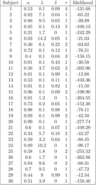
unique maximum, we select the set of parameter with the smallest ri as this parameter appears to be the unique source of non-uniqueness. Hence, we start by fitting the model to determine the set of best parameter values
n
( ˆαi, ˆλi, ˆδi, ˆri) o
for each individual i.12 We then consider a population of 1000 artificial agents with parameters randomly drawn (with replacement) from this set and we compare the simulated outcomes to those observed in terms of individuals’ discovery times and total payoffs.
Figure 3 displays the observed and simulated cumulative distributions (solid and dashed thin lines, respectively) of discovery times and total payoffs. Two-tailed Kolmogorov-Smirnov (KS) tests do not reject the null of the stochastic equivalence of simulated and observed discovery times (p = .382) and total payoffs (p = .304), so that the model fits remarkably well the distributional properties of these variables.13 To put the goodness-of-fit of this pattern-learning model into perspective, we compare it to the one of a constrained version that disactivates the agent’s ability to recognize patterns and consequently use conditional strategies. This is achieved by imposing ri> 200 (the number of rounds of play) which amounts to assuming that the agent never becomes aware of the existence of a temporal payoff structure and thus never uses conditional strategies. We
12
See Appendix C for the list of the obtained set of best parameter values and associated likelihood for each of the subjects.
13
The tests were conducted with ‘one-sample’ KS tests which assumed for theoretical distribution the one of simulated data. Clearly, doing so means that the independence assumption of observed and simulated samples is not satisfied and that the test outcomes should be taken with caution.
Discovery Time Total Payoff æ æææ æææ ææææ æ æ ææ æ æ æ æ æ æ æ æ æ æ æ æ æ æ æ æ æ æ 0 50 100 150 200t ` 0.0 0.2 0.4 0.6 0.8 1.0CDF æ æææ æ æææ æææ æ æ æ æææ æ æ æææ æææ æææ ææææ æ 0 50 100 150 200SΠ 0.0 0.2 0.4 0.6 0.8 1.0CDF
Exp: 133.23 (73.0), Sim: 133.16 (63.45) Exp: 119.06 (50.20), Sim: 117.82 (43.53)
p=0.382 p= 0.304
Figure 3: CDFs of discovery times and total payoffs. Legend: Observed (thin solid with makers), Simulated baseline model (thin dashed), and Simulated constrained model (thick solid). Mean (standard deviation) for observed and simulated baseline model are also shown. P-values are based on Kolmogorov-Smirnov, two-tailed.
fit this constrained version by searching for each individual i the set of best parameters n
( ˜αi, ˜λi) o
. The resulting plots of the simulated distributions in Figure 3 (solid thick lines) clearly indicate no discovery within 200 repetitions and consequently lower payoffs than those observed or simulated by our baseline model.
5
Learning from others
We now extend our baseline treatment and model to allow for and accommodate observational learning. Before spelling out the models, we briefly observe that when compared to the baseline NI treatment, the provision of end-of-round information feedback about an other’s choices, payoffs or both (i.e., the CI, PI or CPI treatments, respectively) considerably affected the participants’ dicovery times and payoffs, but not uniformly so. In each treatment, a few pairs of participants still never discovered the hidden pattern whereas in a few others, one participant discovered it whilst the other did not. Yet, in other pairs, both participants eventually discovered patterns. As in the NI treatment, a few participants who discovered the pattern occasionally deviated from it in subsequent rounds but in contrast to the NI treatment, we find no evidence of participants
settling into more complex and less profitable choice patterns. Appendix D reports the time-series of choices and payoffs for four pairs of participants in the three additional information treatments considered.
5.1 Three observational pattern-learning models
We present three extensions of our baseline pattern-learning model that allow for observational learning. The three extensions assume that agents keep track not only of their own choices and payoffs over time but also part of, or all of the other’s, and thus learn on the basis of these two information sets. However, as the assumption that agents pay equal attention to their own outcomes as to the other’s outcomes has been challenged in the experimental literature (see, e.g., McElreath et al., 2005; Bayer and Wu, 2016), we assume that agent i pays attention to (ai, πi) for sure and pays attention to (aj, πj) with probability qi ∈ [0, 1].14 Let Γi
t= 1 represent i paying attention to
(ajt, πtj) in round t (which happens with probability qi) and Γit= 0 otherwise.
5.1.1 The ‘Choice & Payoff Information’ (CPI) case
Let Ait(a) summarize, at the beginning of round t, the past experience for agent i from choosing option a. Let Ai0(a) = 0.5 for all i and a. We assume that Ait(a) evolves as follows:
Ait+1(a) = αiAit(a) + (1 − αi)πit if a = ait αiAit(a) + (1 − αi)πjt if a = ajt and Γit= 1 Ait(a) otherwise (3)
Compared to the baseline model, Eq. (3) shows that Ai
t(a) is updated not only with the payoff
i obtained for the option he chose (the first line), but also with the option chosen by j and its associated payoff if i paid attention to this additional piece of information. Note also that Eq. (3) allows the Ait(a) to be updated twice in the same period when ait = ajt and Γit= 1. This is based
14
Note that keeping track of whether participants pay attention to the other’s outcomes or not (for example by displaying the information proviso a mouse-click) might provide an estimate of q or allow some modelling of how it changes over time. However, since accessing this information does not guarantee that the participant factors it in
on the assumption that two pieces of the same information has stronger impact than a single piece of information. Just as in the baseline model, we assume that i will choose an option a based on Ait(a) according to Eq. (1).
Now let’s consider how agent i becomes aware of inter-temporal dependencies. We assume, just as in the baseline model, that agent i becomes aware of inter-temporal dependencies when i observes the same sequence of (choice, payoff) pairs. However, this sequence of (choice, payoff) pairs can now be based not only on the sequence of his own (choice, payoff) pairs but also on the observed sequence of j’s (choice, payoff) pairs as long as Γik = Γik−1 = 1. For example, assume li = 2 and ri = 2. Then, as we have noted above, after observing the (choice, payoff)-sequence
{(1, 1), (1, 0)} twice, agent i will start considering the existence of a dependency. Here this sequence of {(1, 1), (1, 0)} can be based on i own choices and payoffs, but also from j’s sequence as long as i paid attention to j’s choice and payoff for two consecutive rounds.
Let us know describe how i’s attractions for conditional strategies are updated. Let Biτ(a|h) = Aiτ(a) for all h at round τ when i became aware of the inter-temporal dependencies. We assume, after round τ , that Bti(a|h) evolves as follows:
Bt+1i (a|h) = βiBit(a|h) + (1 − βi)πti if a|h = ait|hi t−1
βiBit(a|h) + (1 − βi)πtj if a|h = ajt|hjt−1 and Γit= Γit−1= 1 Bi
t(a|h) otherwise
(4)
The first line of (4) stands for period t’s attraction of the conditional strategies being updated on the basis of the resulting payoff. The second line specifies the way the attraction of the observed conditional strategy used by j is updated. For this to operate, i has to pay attention to j’s choices and payoffs in both period t and t − 1, which are captured by the condition Γit = Γit−1 = 1. Note that when ajt|hjt−1= ait|hi
t−1 the same conditional strategy is updated twice in the same period just
Based on Bit(a|h), the choice of option a for agent i in round t is thus be defined as: P r(ait= a|hit−1, hjt−1) = e λitBti(a|hit−1)+ Γi t−1e λi tBti(a|h j t−1) P ke λi tBit(k|hit−1)+ Γi t−1 P ke λi tBti(k|h j t−1) (5)
Note that there are two components in Eq. (5). One is based on own history hit−1, and another is based on the observed history hjt−1. Note that the latter is effective only when i has paid attention to j’s choice and payoff in period t − 1 (i.e., Γit−1= 1). Because if i has not paid attention to what j did (i.e., Γit−1= 0), i has no information about hjt−1. When Γit−1= 1 and hit−16= hjt−1, on the other hand, i can consider conditional strategies based on hi
t−1as well as those based on h j
t−1. Therefore,
each of four possible choices can be generated from two conditional strategies.
5.1.2 The ‘Payoff Information’ (PI) case
The basic idea here is that when i observes j obtaining a sequence of payoff 1s, i tries to figure out how j is obtaining such a stream of high payoffs based on (1) what i knows about the set of possible (choice, payoff) pairs and (2) their inter-temporal dependencies. On the one hand, if i is not yet aware of the existence of the inter-temporal dependencies and conditional strategies, we assume that by observing j’s sequence of high payoffs, i becomes aware of the existence of such dependencies and strategies in addition to the process that we have described in our baseline model based on sequences of agent’s own choice-payoff pairs. Adopting the same reasoning as in the case of own experience, we assume that i would need to observe j obtaining a sequence of consecutive πtj = 1 of length li = 2, at least ri times. Note also that i does not pay attention to j’s payoff all the time (we keep the same probabilistic attention process described above), so that we need, in case of li = 2, Γitπtj = Γit=1πjt−1 = 1 at least ri times to become aware of the existence of the inter-temporal dependencies and conditional strategies.
An example may help. Consider the following history of the payoffs received by agent j and of the rounds in which agent i’s paying attention.
t 20 21 22 23 24 25 26 27 28 29 30 31 32 33
πjt 1 1 1 1 1 1 1 1 1 1 1 1 1 1
Γit 0 0 1 1 0 0 1 1 0 1 0 1 1 0
here i observed j obtaining a payoff of 1 in two consecutive rounds three times: in rounds 22-23, 26-27, and 31-32. If ri = 2, we assume that from round 28 on, i will become aware of the existence of inter-temporal dependencies and start updating based on j’s payoff, when i pays attention to it, as well.
Once i is aware of conditional strategies and has just experienced the (choice, payoff) sequence (1, 1), (1, 0), while observed j obtaining payoff of 1 in the same two rounds, then i will infer (assum-ing he already knows that Π(a)i
t = {0, 1} for a ∈ {1, 2, 3} and Π(4)it = {0.3}) that choosing either
2 or 3 instead of 1 after (1, 1) could have generated a payoff of 1. In fact, this type of inference is possible in our set-up only after i obtains a payoff of 1 in the previous round and 0 in the current one.15 Notice also that this means that i will not use the information about j’s payoff when s/he is not using a conditional strategy. We therefore assume that Ait(a) evolves as follows:
Ait+1(a) = αiAit(a) + (1 − αi)πti if a = ait Ait(a) otherwise
On the other hand, if i is already using a conditional strategy16 then,
Bit+1(a|h) = βiBit(a|h) + (1 − βi)πti if a|h = ait|hi t−1 βiBit(a|h) + (1 − βi)1 if h = hit−1, a 6= ait, πti= 0, πit−1= Γit−1πt−1j = Γitπtj = 1, 1 ∈ Πit(a) Bti(a|h) otherwise (6)
Note that we are assuming that j’s payoff information is used only if i has observed that j
15
After receiving a 0 payoff in the previous round, all choices (but 4) can result in both payoff of 0 or 1. 16
As in the baseline and extended model for CPI, we assume that Biτ(a|h) = Aiτ(a) for all h at round τ when i became aware of the inter-temporal dependencies
obtained a payoff of 1 in two consecutive rounds. The additional conditions listed in the second line of Eq. (6) stand for the updating based on observed payoff obtained only when i received payoff of 0 in t, and only for those options that i did not choose in t but i knows that they can generate payoff of 1.
The choice of a conditional strategy in round t will be based on Bti(a|h) just as in the baseline case (Eq. (2)).
5.1.3 The ‘Choice Information’ (CI) case
Here, intuitively, the decision will involve mimicking. However, we will implement it through the evolution of attractions to keep the modeling framework consistent across our four conditions instead of modeling it directly as agents copying the observed choice patterns. The basic idea will be that when agent i detects a pattern in the choices made by j, he will assume that j is doing so because it generates a high payoff. Thus, the attraction for conditional strategies will be updated with “presumed” high payoffs based on i’s observation about j’s choices (of course, given i’s knowledge about the set of possible payoffs for each option and conditional choices). This process operates in addition to the learning process described in our baseline model.
First i has to recognize patterns in j’s choices. He does so when he observes that j has been making the same sequence of li consecutive choices, among three options other than 4, ri times in the row.17 Say i has observed j making the sequence of choices 3 → 2 twice in a row “recently.” Here “recently” is defined as being among those recent blocks of two consecutive rounds in which i has paid attention to what j has chosen and j has chosen 3 in the first round of a block. If i has already become aware of inter-temporal dependencies, this will translate into i assuming that strategy 2|(3, 1) will result in payoff of 1.
Again, an example may help. Consider the following history of choices made by agent j and of the rounds in which i was paying attention to it.
17
Excluding the sequence of choices involving 4 is specific to our experimental set up. We do so here because we assume that agents will quickly learn that choosing 4 results in the sure payoff of 0.3.
t 20 21 22 23 24 25 26 27 28 29 30 31 32 33
ajt 2 1 3 2 1 3 2 1 3 2 1 3 2 1
Γit 0 0 1 1 0 0 1 1 0 1 0 1 1 0
In this example, j is assumed to be following the best choice sequence in the setup, and i has paid attention to j’s choice in rounds 22, 23, 26, 27, 29, 31, and 32. Of the three blocks of two consecutive rounds in which i paid attention, i.e., 22-23, 26-27, and 31-32, both the first and the last ones contain the choice sequence of (3, 2) by j. This will induce i to start making inferences about the conditional strategy 2|(3, 1).
In the case where i has not yet become aware of conditional strategies, then the first time i notices the pattern in j’s choice sequences, we assume that i then becomes aware of the existence of such strategies and starts learning about their performance.
Recall, however, that i does not observe j’s payoff directly. Thus, we assume that when i is making unconditional choices, the observation of j’s choice will not be used in the evolution of Ait(a).
Putting all these assumptions together, the observation of j’s choice will be used only in the evolution of Bt+1i (a|h) as follows:
Bt+1i (a|h) = βiBit(a|h) + (1 − βi)πti if a|h = ait|hi t−1
βiBit(a|h) + (1 − βi)1 if a|h = (ajt|(ajt−1, 1)), Γit= Γit−1= 1, ajt ∈ {1, 2, 3}, except when ait|hi t−1= a j t|(a j t−1, 1) and πti 6= 1 Bti(a|h) otherwise (7)
The first line of (7) is the same in all the models because it does not involve observation of j’s choice. The second line stands for the updating based on the choices made by j. For this to operate, we require Γit= Γit−1= 1, i.e., that i pays attention to j’s choice in two consecutive rounds. Furthermore, as one can see from the condition (ajt−1, 1) which requires the payoff associated with ajt−1 to be 1, we are excluding the case where ajt−1 = 4 because by the time agents are aware of
conditional strategies, they must have learned that option 4 will always result in payoff of 0.3. This also explains why we are restricting our attention to ajt ∈ {1, 2, 3}. Note that we impose one more condition, namely that ait|hi
t−1 = a j t|(a
j
t−1, 1) and πti 6= 1, for not updating the attraction of
ajt|(ajt−1, 1). The reason is obvious: if i and j chose the same conditional strategy, and i’s payoff is different from 1, i should infer that j’s payoff is also different from 1.
Finally, the choice of a conditional strategy in round t will be based on Bti(a|h) just as in the baseline case (Eq. (2)).
5.2 Simulation results
We simulate the above models using the set of parameter values n
( ˆαi, ˆλi, ˆδi, ˆri) o
that best fit the baseline model, and assuming different values for qi= q for all i. That is, for each value of q and for each individual in each of 500 simulated pairs of agents, we randomly draw (with replacement) each of the parameter values from the set of parameters pertaining to the NI treatment. We have chosen to evaluate the goodness-of-fit of our models on the grounds of such out-of-sample predictions to overcome the identification problems that are inherent to the estimation of ten parameters for each pair of participants (i.e., ( ˆαi, ˆλi, ˆδi, ˆri) and qi for each participant).
Figure 4 displays the simulated distributions of discovery times and total payoffs assuming that q = 1 (i.e., agents are assumed to always pay attention to the other’s payoff and/or choice) along with the observed ones. The plots suggest that overall, participants discovered the hidden cycle somewhat faster and earned higher total payoffs than our simulated agents. However, the conduct of two-tailed Kolmogorov-Smirnov tests indicates that differences between observed and simulated data samples are significant at α = 5% for discovery times in the PI treatment and for total payoffs in CPI (p = .028 and p = .008, respectively). Otherwise, our models provide a good out-of-sample fit to discovery times in CPI and CI and to total payoffs in PI and CI as the simulated and observed distributions are then not significantly different at α = 5% (p = .053 and .249 for discovery times, and p = .104 and .581 for total payoffs, respectively).
We proceed with cross-treatment comparisons of the models’ simulations and the observations. The upper panel of Figure 5 displays the simulated distributions of discovery times (left panel)
CPI
Discovery Time Total Payoff
ò òòò ò òòò òòòò ò òòò òòò òòò ò ò òòò òò ò ò ò ò ò ò 0 50 100 150 200t ` 0.0 0.2 0.4 0.6 0.8 1.0CDF ò òòò ò ò ò òò òòòò òòò òòò òòò ò òòò òòò ò ò òò òò 0 50 100 150 200SΠ 0.0 0.2 0.4 0.6 0.8 1.0CDF
Exp: 75.75 (59.05), Sim: 97.63 (63.02) Exp: 154.07 (42.70), Sim: 138.91 (41.09)
p=0.053 p= 0.008
PI
Discovery Time Total Payoff
ì ììì ììì ì ìì ì ììì ì ììì ì ìì ì ì ìì ì ì ì ì ì ì ì ì ì ì 0 50 100 150 200t ` 0.0 0.2 0.4 0.6 0.8 1.0CDF ì ììì ììì ì ììì ìì ì ìì ìì ì ì ìì ììì ìììì ìììì ìì 0 50 100 150 200SΠ 0.0 0.2 0.4 0.6 0.8 1.0CDF
Exp: 110.13 (76.43), Sim: 117.32 (64.11) Exp: 131.26 (52.55), Sim: 127.98 (42.57)
p=0.028 p= 0.104
CI
Discovery Time Total Payoff
à àà à à àà àààà ààà à à à à à ààà à à àà à à à à à à à à à 0 50 100 150 200t ` 0.0 0.2 0.4 0.6 0.8 1.0CDF à ààà ààà à à à ààà à ààà à àà à à ààà ààà ààà àà à à 0 50 100 150 200SΠ 0.0 0.2 0.4 0.6 0.8 1.0CDF
Exp: 106.38 (64.70), Sim: 117.27 (63.66) Exp: 131.96 (43.92), Sim: 128.07 (42.47)
p=0.249 p= 0.581
Figure 4: CDFs of discovery times and total payoffs.
Legend: Observed (solid), Simulations under qi= 1.0 for all i (dashed). Mean (standard deviation) are also shown. P-values are based on KS test, two-tailed.
Model simulation
Discovery Time Total Payoff
0 50 100 150 200t ` 0.0 0.2 0.4 0.6 0.8 1.0CDF 0 50 100 150 200SΠ 0.0 0.2 0.4 0.6 0.8 1.0CDF Experiments
Discovery Time Total Payoff
æ ææ æ ææ æ æ æ ææ æ ææ æ æ æ æ æ æ æ æ æ æ æ æ æ æ æ æ æ æ æ à àà à à à àà àà àà àà àà à à à à à àà à à à à à à à à à à à à ì ìì ìì ì ì ìì ìì ìì ì ì ìì ìì ìì ì ì ìì ì ì ì ì ì ì ì ì ì ì ò òò òò òò ò òò òò òò òò òò òò òò òò òò òò ò ò ò ò ò ò ò 0 50 100 150 200t ` 0.0 0.2 0.4 0.6 0.8 1.0 CDF æ NI à CI ì PI ò CPI æ ææ ææ æ æ æ ææ æ æ æ æ æ ææ æ æ ææ ææ ææ ææ ææ ææ ææ à àà àà àà à à à à àà àà àà àà àà à àà àà àà àà à àà à à ì ìì ìì ìì ì ì ìì ìì ì ì ìì ì ìì ìì ìì ìì ìì ìì ìì ììì ò òò òò ò ò òò òò òò òò òò ò òò òò ò òò ò òò òò òò òòò 0 50 100 150 200SΠ 0.0 0.2 0.4 0.6 0.8 1.0 CDF æ NI à CI ì PI ò CPI p = 0.033 (KW) p = 0.025 (KW) p-values CI PI CPI NI 0.065 0.114 0.001 CI 0.585 0.027 PI 0.025 p-values CI PI CPI NI 0.141 0.176 0.003 CI 0.522 0.023 PI 0.031
Figure 5: CDFs of discovery times and total payoffs (with p-values of Kruskal-Wallis tests for multiple sample comparisons and Fisher-Pitman permutation tests for pair-wise comparisons (one-tailed)).
Legend: NI (Thick dashed blue), CPI (Thick solid red), PI (Thin dashed orange), CI (Thin solid light blue).
and total payoffs (right panel), assuming q = 1, whereas the lower panel displays the observed distributions along with the outcomes of Kruskal-Wallis (KW) and Fisher-Pitmann permutation tests (for independent samples) that assess their stochastic equivalence.18 There are two things worth noting here. First, the simulated distributions clearly confirm the conjecture that the more items of information one has about the other participant, the faster the hidden pattern will be discovered and the higher the total payoffs will be. This is confirmed by the observed distributions and test statistics for the NI and the CPI treatments but not by those of the partial information treatments CI and PI which are not significantly different from the NI treatment (p-values > 0.05). Second, the simulated distributions for the CI and PI treatments are virtually identical and the observed ones are not significantly different which suggests that the type of information received about the other participant does not significantly affect the variables of interest. In the light of Sonsino (1997)’s claim that the repeated observation of the same pattern of choices over a long period of time must be recognized by the observer (cf. Footnote 3), these findings raise the question as to whether observing the others’ choices is cognitively equivalent to observing the other’s payoff outcomes. On the one hand, the lack of significant difference between the simulated distributions of the CI and PI treatments and the empirical support of this prediction suggest that this is indeed the case. However, as we noted when presenting the pattern-learning model for the PI treatment, one could argue that observing another’s payoff pattern is not as informative as observing another’s choice pattern since the latter immediately calls for an imitation of such behaviour that might lead to the discovery of the hidden pattern. This is offset by the fact that observing a series of payoffs of 1, for example, reveals that there is a pattern of actions which leads to these high payoffs and thus stimulates the individual to search for such a pattern. This, in turn, would suggest that, if there is an informational difference, our observational pattern-learning model fails to capture it. On the other hand, the lack of significant difference between the observed distributions of CI and NI and of PI and NI suggest that the provision of information on past choices or past payoffs is in fact not sufficient to facilitate pattern-discovery in our framework. Here we recall that our descriptive data analyses indicated a considerable heterogeneity in subjects’ behaviour which, in turn, may have
18
interfered with our predictions.
5.3 Does observation facilitate discovery?
Although it is quite intuitive that observing the choices and/or payoffs of another person who has discovered the hidden pattern should help an observer who has not yet found the pattern, it is less clear whether observing the choices and/or payoffs of another participant who has not found any pattern is equally helpful. We investigate this by first identifying in each pair of simulated agents, the one who discovered the hidden pattern first, henceforth the Early finder, or second, henceforth the Late finder. If the hidden pattern was not discovered, then the labels are randomly assigned. For the baseline treatment, we randomly match agents in pairs and assign labels by comparing their respective discovery times so as to get some benchmark for Early and Late finders who do not observe any other agent’s outcome(s).
Figure 6 shows the distributions of discovery times of each type of simulated agents for four values of q ∈ {0.4, 0.6, 0.8, 1}.
The simulations suggest that if q = 1 (as we assumed above), the distributions of discovery times for both Early and Late finders will be ordered as CPI < CI ≈ PI < NI. However, for lower values of q such as q = 0.6, the distributions of discovery time for the Early finders in the information treatments (CI, PI, CPI) become similar, while those of Late finders maintain the same ordering as when q = 1. And if q = 0.4, the discovery times of Early finders are basically the same across treatments whereas for Late finders, only CPI results in a markedly earlier discovery compared to the other treatments.
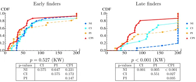
We proceed by displaying the observed distributions of discovery times of Early and Late finders in Figure 7. The plots and KW test statistics for Late finders indicate that they greatly benefited from the additional information; just as in our simulations with q ≥ 0.6. Those in CPI benefited most and significantly more than those in CI or PI whose distributions are not significantly differ-ent. When compared to NI, the plots and test statistics also indicate that the partial information feedback of these treatments significantly improved their discovery times. Interestingly, the ob-served distributions of Late finders in CI also suggest that when compared to PI, discovery times
q = 1.0
Early finders Late finders
0 50 100 150 200t ` 0.0 0.2 0.4 0.6 0.8 1.0CDF 0 50 100 150 200t ` 0.0 0.2 0.4 0.6 0.8 1.0CDF q = 0.8
Early finders Late finders
0 50 100 150 200t ` 0.0 0.2 0.4 0.6 0.8 1.0CDF 0 50 100 150 200t ` 0.0 0.2 0.4 0.6 0.8 1.0CDF q = 0.6
Early finders Late finders
0 50 100 150 200t ` 0.0 0.2 0.4 0.6 0.8 1.0CDF 0 50 100 150 200t ` 0.0 0.2 0.4 0.6 0.8 1.0CDF q = 0.4
Early finders Late finders
0 50 100 150 200t ` 0.0 0.2 0.4 0.6 0.8 1.0CDF 0 50 100 150 200t ` 0.0 0.2 0.4 0.6 0.8 1.0CDF
Figure 6: CDFs of the simulated discovery times of Early and Late finders for three values of q for all the treatments. q = 1.0 (1st row), q = 0.8 (2nd row), q = 0.6 (3rd row), and q = 0.4 (4th row).
Early finders Late finders æ æ æ æ æ æ æ æ æ æ æ æ æ æ æ æ æ æ à à à à à à à à à à à à à à à à à à à ì ì ì ì ì ì ì ì ì ì ì ì ì ì ì ì ì ì ì ò ò ò ò ò ò ò ò ò ò ò ò ò ò ò ò ò ò ò 0 50 100 150 200t ` 0.0 0.2 0.4 0.6 0.8 1.0 CDF æ NI à CI ì PI ò CPI æ æ æ æ æ æ æ æ æ æ æ æ æ æ æ æ æ æ à à à à à à à à à à à à à à à à à à à ì ì ì ì ì ì ì ì ì ì ì ì ì ì ì ì ì ì ì ò ò ò ò ò ò ò ò ò ò ò ò ò ò ò ò ò ò ò 0 50 100 150 200t ` 0.0 0.2 0.4 0.6 0.8 1.0 CDF æ NI à CI ì PI ò CPI p = 0.527 (KW) p < 0.001 (KW) p-values CI PI CPI NI 0.575 0.647 0.221 CI 0.575 0.172 PI 0.147 p-values CI PI CPI NI 0.001 0.005 < 0.001 CI 0.551 0.027 PI 0.035
Figure 7: CDFs of discovery times of Early and Late finders in the experiments (with p-values of Kruskal-Wallis tests for multiple sample comparisons and Fisher-Pitman permutation tests for pair-wise comparisons (one-tailed)).
Legend: NI (Thick dashed blue), CPI (Thick solid red), PI (Thin dashed orange), CI (Thin solid light blue).
sharply decrease from round 110 onwards which is in line with the conjecture that the CI treatment should make it easier to discover the pattern once the other has discovered it and exhibits a cyclical choice pattern. As for the Early finders, we find no significant difference across treatments, as in our model simulation for q ≤ 0.6, so that the additional information provided had no significant effect on their performance.
To further determine who benefited most from the information provided, we track the evolution of average payoffs of Early and Late finders in each treatment. Figure 8 reports their respective median of round average payoffs for each batch of 10 rounds in each treatment. The plots and KW test statistics suggest that round average payoffs are not significantly different across treatments for the first five batches and are actually very similar across types (i.e., Early and Late). Differences emerge from the sixth batch onwards: the round average payoffs of Late finders vary widely across treatments whereas those of Early finders become identical. This confirms that the information provided did not affect Early finders whereas it significantly helped Late finders. Note also that the median average round payoffs in CI sharply increase between the eleventh and fifteenth batch,
Early participants Late participants ææ æ æ æ æ æ æ æ æ æ æ æ æ æ æ æ æ æ æ à àà à à à à ààà à à à à à à à à à à ì ì ì ì ì ì ì ì ì ì ì ì ì ì ì ì ì ì ì ì ò ò ò òò ò ò ò ò ò ò ò ò ò ò ò ò ò ò ò 0 5 10 15 20Τ 0.2 0.4 0.6 0.8 1.0 Median <Π> æ NI à CI ì PI ò CPI ææ æ æ æ æ æ æ æ æ æ æ æ æ æ æ æ æ æ æ à ààà à ààà àà à à à à à à à à à à ì ì ì ì ì ì ì ì ì ì ì ì ìì ì ì ì ìì ì ò òòò ò ò ò ò ò ò ò ò ò ò ò ò ò ò ò ò 0 5 10 15 20Τ 0.2 0.4 0.6 0.8 1.0 Median <Π> æ NI à CI ì PI ò CPI
p-values from Kruskal-Wallis test
τ 1 2 3 4 5 6 7 8 9 10 Early participants 0.249 0.709 0.814 0.416 0.801 0.288 0.430 0.261 0.852 0.300 Late participants 0.098 0.204 0.592 0.067 0.981 0.008 0.044 0.039 0.004 0.018 τ 11 12 13 14 15 16 17 18 19 20 Early participants 0.126 0.317 0.638 0.852 0.693 0.759 0.690 0.511 0.885 0.676 Late participants 0.003 0.019 0.014 0.005 0.014 0.012 0.008 0.032 0.010 0.054
Figure 8: Dynamics of median round average payoff (over block of 10 rounds) of Early and Late participants (with p-values of Kruskal-Wallis tests).
which is again in line with the claim that discovering a pattern is easier as a Late finder in CI than in PI because one can simply copy the systematic behavior of the Early finder.
To this extent, the models’ general prediction (with q < 1) that the more information about the other participant’s last decision and/or reward accelerates discovery appears to hold mainly for Late finders, and the conjecture that it should be even faster in CI than in PI seems to hold only once Late finders accumulated some experience of the game they were playing. So we have a partial answer to the relative speed of discovery in CI as opposed to PI which we discussed earlier but which is not directly incorporated in our model.
6
Conclusion
We report on a series of bandit experiments that manipulate the end-of-round information feedback to assess the effect of observational learning on the discovery of the bandits’ hidden payoff structure. We considered four treatments, each involving four options and consisting of 200 rounds of play. The payoffs of the first three options have an undisclosed deterministic temporal structure which generates a payoff of 1 in each round, provided that the options are chosen in the right sequence,
whereas the fourth generates a sure payoff of 0.3.
In a baseline treatment (NI), participants played in isolation, i.e., with no information on other’s play or outcomes. While some participants were surprisingly fast in “discovering” the hidden mechanism in this treatment, half of them failed to do so by the end of the experiment. Most participants initially explored among four different options. At some point, however, those who were successful seem to have had an “aha” moment, and started to reinforce on sequences of actions taken in the past. We propose a simple reinforcement model that captures such pattern-learning and find that it reproduces the distributional properties of the observed discovery times and total payoffs remarkably well.
In the three other treatments, participants were randomly matched in fixed pairs and received information on the other’s last choice (CI), the other’s last payoff (PI) or on both the other’s last choice and payoff (CPI). These treatments allow us to assess the effect of observational learning on the participants’ discovery of the bandits’ payoff pattern and the data confirms earlier findings pertaining to game theoretic settings that the provision of information on both the other’s last choice and payoff accelerates discovery most whereas the provision of partial information (i.e., the other’s last choice or last payoff) does not when compared to the baseline treatment (NI). We extend our basic model to capture the behaviour observed in these treatments and find that the discovery times are well supported by out-of-sample predictions in the partial information treatments but not in CPI where participants performed even better than predicted. Such a gap between predictions and observations in this treatment may be evidence for a compounding effect of information that is not captured by our model. On the other hand, the irrelevance of the type of information (choice or payoff) for the participants’ discovery times in CI and PI may result from their heterogeneous traits. We therefore identify Early and Late finders within each pair and find that the information provided significantly improves the discovery times of Late finders in all three treatments while leaving those of Early finders largely unaffected. This is supported by the model’s out-of-sample predictions and/or by an ex post adjustment of the probability of paying attention to the other’s outcome(s).
with and without observational learning. We believe that it relates to the recent investigations of Dufwenberg et al. (2010) and McKinney and Van Huyck (2013) which focused on solving a well-defined problem which have a “solution” and involve an “aha” moment or, referring to Archimedes, the “eureka” moment when an individual suddenly perceives the answer to a problem s/he has been wrestling with. In our context, the analogy to finding a solution is when participants believe they have discovered the pattern and start exploiting it.19 Our approach could be refined and stress-tested with further experiments that would control the size (or presence) of the safe bandit-option, the hidden payoff pattern and/or the length of the game’s history provided in the information treatments. We hope that our contribution will open the way to answering a number of questions that arise when individuals are trying to learn how to act in an unknown environment.
References
Agarwal, A., D. Hsu, S. Kale, J. Langford, L. Li, and R. E. Schapire (2014): “Taming the monster: A fast and simple algorithm for contextual bandits,” in In Proceedings of the 31st International Conference on Machine Learning (ICML-14), 1638–1646.
Armantier, O. (2004): “Does observation influence learning?” Games and Economic Behavior, 46, 221–239.
Arrow, K. J. and J. R. Green (1973): “Notes on Expectations Equilibria in Bayesian Settings,” Working Paper 33, Institute for Mathematical Studies in the Social Sciences, Stanford University.
Auer, P. (2002): “Using Confidence Bounds for Exploitation-Exploration Trade-offs,” Journal of Machine Learning Research, 3, 397–422.
19
Our investigation also relates to recent research in the neurosciences which investigates which are the mental processes at work that lead individuals to learn how to understand and operate in their environment. There, it is argued that different mechanisms operate in the brain when an individual switches from exploiting the information about the various options he has tried to exploring new ones (see Cohen et al., 2007; Laureiro-Mart´ınez et al., 2014, 2015). The authors compared two groups of subjects, managers and entrepreneurs, and found that the threshold at which a manager passed to exploration is significantly higher than that of an entrepreneur. In other words, entrepreneurs tend to function in the exploratory mode more often than managers. Indeed, the distinction that emerges between people with different professions suggests that this process is also present in longer term situations.